The relative concentration of visible and dark matter in clusters of galaxies

Abstract

In general, the best evidence for the presence of dark matter is obtained when an additional mass component with distribution different from that of the visible matter is needed to explain the dynamical data. Here we wish to study the relative distribution of visible and dark matter in clusters of galaxies, in comparison with the distribution observed on the galactic scale; in particular, we wish to check whether dark matter is more concentrated than visible matter without using assumptions or other constraints deriving from cosmology. We also intend to check whether the result depends significantly on the dynamical state of the cluster under investigation. We consider two clusters (A496 and Coma) that are representative of the two classes of cool-core and non-cool-core clusters. We first refer to a two-component dynamical model that ignores the contribution from the galaxy density distribution and study the condition of hydrostatic equilibrium for the hot intracluster medium (ICM) under the assumption of spherical symmetry, in the presence of dark matter. We model the ICM density distribution in terms of a standard $\beta$-model with $\beta=2/3$, i.e. with a distribution similar to that of a regular isothermal sphere (RIS), and fit the observed X-ray brightness profiles. With the explicit purpose of ignoring cosmological arguments, we naïvely assume that dark matter, if present, has an analogous density distribution, with the freedom of two different density and length scales. The relative distribution of visible and dark matter is then derived by fitting the temperature data for the ICM under conditions of hydrostatic equilibrium. For both clusters, we find that dark matter is more concentrated with respect to visible matter. We then test whether the conclusion changes significantly when dark matter is taken to be distributed according to cosmologically favored density profiles and when the contribution of the mass contained in galaxies is taken into account. Although the qualitative conclusions remain unchanged, we find that the contribution of galaxies to the mass budget is more important than generally assumed. We also show that, without resorting to additional information on the small scale, it is not possible to tell whether a density cusp is present or absent in these systems. In contrast with the case of individual galaxies, on the large scale in clusters of galaxies dark matter is indeed more concentrated than visible matter.

1 Introduction

Dark matter is known to play a significant role on the scale of galaxies and to dominate on the scale of clusters of galaxies.

On the galactic scale, for both spirals and ellipticals, the contribution of dark matter to the total mass generally exceeds 50%. Typically, the dark component is diffuse, i.e. it becomes more important at large radii (e.g., see Bertin [1]). This is the reason why in galaxies it is usually referred to as a dark matter “halo”.

On the larger scale of clusters of galaxies, it is generally stated that dark matter represents about 85% of the total mass and that the visible matter is mostly in the form of a hot intracluster medium (ICM) (for some estimates see, e.g., Mohr et al. [2]; Ettori et al. [3]; Rosati et al. [4]). Much work has been done to study how this fraction changes with radius (e.g., David et al. [5]; White & Fabian [6]; Ettori & Fabian [7]; Vikhlinin et al. [8]; Allen et al. [9]).

In this paper, we wish to study the relative distribution of dark and visible matter in clusters of galaxies in the most simple dynamical framework. On purpose, we will ignore any suggestion or constraint from the cosmological context and proceed by applying a most naïve and simple parametric dynamical model to the hot ICM, considered to be in hydrostatic equilibrium.

The work presented here is based on the use of X-ray data from BeppoSAX, which are well suited for the discussion of the mass distribution on the large scale, at least out to a scale close to 1 Mpc. Clearly, for the discussion of the mass distribution on the small scale of the inner sphere of radius $\approx$ 100 kpc, other data (X-ray data from Chandra, strong lensing, or stellar dynamical data for the bright central galaxy often present) would provide the decisive pieces of information but would also require a much more sophisticated modeling (see Mahdavi et al. [10]). Most likely, in order to make a significant statement beyond the scale of 1 Mpc, different diagnostics, such as that offered by the Sunyaev-Zel’dovich effect, will be required.

The paper is organized as follows. In Sect. 2 the simplest dynamical model (in which the contribution of the mass associated with galaxies is ignored) is introduced. The results are presented in Sect. 3 and discussed in Sect. 4. The contribution of the mass associated with galaxies is discussed in Sect. 5. In Sect. 6 the conclusions are drawn.

To quantify the scales of the density distributions in the two clusters considered, except where explicitly noted, we refer to the following value of the Hubble constant: $H_{0}=50\rm{\ km\ s^{-1}\ Mpc^{-1}}$. This is equivalent to setting $h=0.5$, where $h$ denotes the Hubble constant in units of $100\rm{\ km\ s^{-1}\ Mpc^{-1}}$. This choice is rather common within the X-ray astrophysics community. In Sect. 4 we comment on the consequences of adopting the currently favored value $h=0.7$.

2 The simplest dynamical model

Even if the morphology of galaxy clusters is quite complex, we adopt spherical symmetry for the ICM, on the scales considered. We assume hydrostatic equilibrium and a local ideal equation of state, i.e. we ignore the possible presence of turbulent pressure. We study a model with only two components, i.e. the intracluster medium and the dark matter. For simplicity, the contribution of galaxies is neglected. Strictly speaking, what we call dark matter in our model, being the difference between total and ICM matter, also includes the contribution of some visible mass. In practice, given our focus on the large-scale distributions, our simplified notation is appropriate. We will return on this issue in Sect. 5, where we discuss the mass contribution associated with the galaxies.

Starting from these hypotheses, we now proceed to describe how a dynamical model can be constructed so that the relative mass distribution in clusters of galaxies can be derived from the X-ray data. First of all, we extract the ICM radial density profiles by fitting the electron density distribution (associated with the X-ray brightness profiles) with a $\beta$-model (Cavaliere & Fusco-Femiano [11]).

We take (e.g., see Voit [12] and references therein) $\beta=2/3$ and express the radial coordinate in dimensionless form as $x=r/r_{X}$ so that our fitting formula can be written as

$$\rho_{X}(x)={\rho_{X}}^{(0)}\left(1+x^{2}\right)^{-1}\ ;$$ (1)

here ${\rho_{X}}^{(0)}$ and $r_{X}$ are the density and the length scales. Note that this is often used as a simple representation of the density profile of a self-gravitating regular isothermal sphere (RIS).

We then consider the hydrostatic equilibrium equation

$$\frac{k}{\mu m_{p}}\frac{1}{\rho_{X}(r)}\frac{d}{dr}\left[\rho_{X}(r)T_{X}(r)\right]=-\frac{GM_{tot}(r)}{r^{2}}\ ,$$ (2)

where $T_{X}(r)$ is the value of the ICM temperature at a given distance $r$ from the center of the cluster and $M_{tot}(r)$ is the total mass of the system at radius $r$

$$M_{tot}(r)=4\pi\int_{0}^{r}\left[\rho_{X}(r^{\prime})+\rho_{DM}(r^{\prime})\right]r^{\prime 2}dr^{\prime}=M_{X}(r)+M_{DM}(r)\ .$$ (3)

Here $\rho_{DM}(r)$ is identified with the dark matter density profile. We may then introduce the quantity

$$f_{gas}(r)=\frac{M_{X}(r)}{M_{tot}(r)}\ ,$$ (4)

which represents the gas fraction and is an increasing function of radius if dark matter is more concentrated with respect to visible matter.

To test whether dark matter is more or less concentrated with respect to visible matter, we adopt the simplest form for the dark matter density profile, i.e. the approximate representation of a regular isothermal sphere (RIS),

$$\rho_{DM}(x)={\rho_{DM}}^{(0)}\left[1+\left(\frac{x}{\lambda}\right)^{2}\right]^{-1}\ ,$$ (5)

where we have introduced a “concentration parameter” $\lambda=r_{DM}/r_{X}$. If the fitting procedure will yield values of $\lambda$ smaller or larger than unity, i.e. values of $r_{DM}$ smaller or larger than $r_{X}$, we will say that dark matter is more or less concentrated, respectively.

For comparison, we will also refer to a NFW profile (Navarro et al. [13]), which we express as

$$\rho_{NFW}(x)=\frac{{\rho_{NFW}}^{(0)}}{(x/\lambda_{c})(1+x/\lambda_{c})^{2}}\ .$$ (6)

Note that $\lambda_{c}$ is not a direct measure of the dark matter concentration, because the $\beta$-model for the ICM and the NFW profile for the dark matter have different analytical forms. Since the models considered (Eq. (1), Eq. (5), and Eq. (6)) generate mass profiles that diverge at large radii, we introduce a cutoff radius $r_{out}=ar_{X}$ (to be interpreted as the outermost radius for which observational X-ray temperature and brightness data are available). We thus introduce the parameter f as the visible-to-dark mass content ratio over the whole cluster volume defined by $r_{out}$:

$$\int_{0}^{ar_{X}}\rho_{X}(r)r^{2}dr=\textsf{f}\int_{0}^{ar_{X}}\rho_{DM}(r)r^{2}dr\ .$$ (7)

In this way the dimensional scales of the dark matter density profile (either Eq. (5) or Eq. (6)) can be expressed through the dimensionless parameters $\lambda$ and f. In terms of the function $f_{gas}$ introduced in Eq. (4), we thus have $f_{gas}(r_{out})=\textsf{f}/(\textsf{f}+1)$.

The hydrostatic equilibrium equation is then used to derive a theoretical evaluation of the ICM temperature at any given radius, $T_{X}(x,\lambda,\textsf{f})$. This temperature value can be compared to the observed one, $T_{X}^{obs}(x)$. By minimizing

$$\chi^{2}=\sum_{i=1}^{n}\left[\frac{T_{X}^{obs}(x_{i})-T_{X}(x_{i},\lambda,\textsf{f})}{\sigma_{i}^{T}}\right]^{2}\$$ (8)

where $x_{i}$ are the locations where the temperature data are available, $x_{n}=a$, and $\sigma_{i}^{T}$ is the error in $T_{X}^{obs}(x_{i})$, the best-fit values of the parameters $\lambda$ and f are found. Note that, in this approach, we are making no assumptions on the possible existence of a global equation of state (such as the polytropic equation $p\propto\rho^{\gamma}$), which might dictate a given profile $T_{X}$ in correspondence of a given density profile $\rho_{X}$ of the ICM. There is growing consensus that, in the outer regions, the ICM has a declining temperature profile (Markevitch et al. [14]; De Grandi & Molendi [15]; Vikhlinin et al. [16], [8]; Pratt et al. [17]), but here we need not enter the issue of whether this profile has universal character and can be traced to a general equation of state.

2.1 The sample and the data

We have decided to test this method by focusing on two clusters (A496 and A1656, i.e. Coma) which are representative of two classes: cool-core (or relaxed) clusters and non-cool-core (or non-relaxed) clusters. Both clusters belong to the nearby universe, at redshift $z=0.0320$ and $0.0232$, respectively.

For the ICM data, we take those of Ettori et al. [3], where the methods for collecting the data and their deprojection are explained in detail (see also De Grandi & Molendi [18], [15]).

Even if spherical symmetry and hydrostatic equilibrium may be inadequate when dealing with accurate models of specific cases, especially in the case of non-relaxed clusters (for a relatively recent study of the dynamical state of Coma, see Neumann et al. [19]), the two clusters considered in this paper are sufficiently regular to be taken as reasonable test-cases for the application of our simple dynamical model to the study of the relative concentration of visible and dark matter on the large scale.

3 Results

3.1 Electron density profiles

For the electron density profile we follow Eq. (1), with electron density scale $n_{0}$ and obtain the values of the model parameters (the central electron density scale $n_{0}$ and the length scale $r_{X}$) by minimizing

$${\chi}^{2}=\sum_{i=1}^{n}\left[\frac{n_{e}^{obs}(r_{i})-n_{e}(r_{i})}{\sigma_{i}^{n}}\right]^{2}\ ,$$ (9)

where $r_{1}$ is the radius of the innermost bin for which we have a density measure and $n_{e}^{obs}(r_{i})$ is the observed density value at $r_{i}$; $\sigma_{i}^{n}$ is the uncertainity in $n_{e}^{obs}(r_{i})$.

In order to avoid modeling problems concerning the possible presence of turbulent motions or the physics of individual galaxies, we have decided to make a 100 kpc cut in the central regions. This leads to the exclusion of the innermost data point. Therefore, the central density $n_{0}$ is the extrapolation to the center of this fit and should not be taken literally as an estimate of the central electron density.

In Table 1 we report the best-fit values for each cluster; these values are the ones that are used in Subsect. 3.2 to derive the dark matter parameters.

Table 1: Best-fit values for the parameters of the electron density profile (Eq. (1)) for A496 and Coma ($h=0.5$).

Cluster	$n_{0}$	${\rho_{X}}^{(0)}$	$r_{X}$	${\tilde{\chi}}^{2}$	(d.o.f.)
	($10^{-3}\ {\rm{cm}}^{-3}$)	$(10^{14}\ {\rm{M_{\odot}}}\ {\rm{Mpc}}^{-3})$	(Mpc)
A496	4.$910_{-0.060}^{+0.047}$	1.411	$0.182_{-0.002}^{+0.002}$	4.9	(3)
Coma	2.$987_{-0.020}^{+0.018}$	0.8584	$0.410_{-0.002}^{+0.002}$	40.3	(3)

In the third column of Table 1 we record the values of the central mass density of the ICM, converted from the electron density with the relation $\rho_{X}=\mu_{e}n_{e}m_{p}$, with $m_{p}$ the proton mass and $\mu_{e}=1.1696$.

In both cases, but especially for Coma (see also our final comment in Subsect. 2.1), the values of the reduced ${{\chi}}^{2}$, denoted by ${\tilde{\chi}}^{2}$, are quite high: this is due to the fact that the values of $\sigma^{n}$ are small, since the measures of the electron density are very precise. We will use the model and the inferred parameters as a reasonable representation of the electron density in the region outside the central 100 kpc.

3.2 Temperature profiles

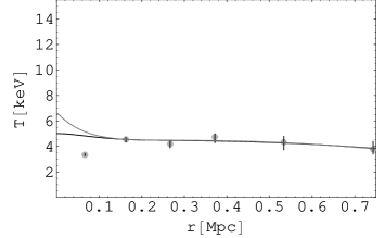
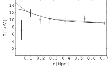
Figure 1: Temperature profiles for A496 (left) and Coma (right) for the RIS model (thick line) and the NFW profile (thin line). The circles are the data with the error bars; for both clusters, the innermost data point is inside the 100 kpc cut region, so it is excluded from the fit. The figure is based on $h=0.5$.

Based on the input parameters obtained in Subsect. 3.1, we have proceeded to apply the method described in Sect. 2. The temperature profiles are illustrated in Fig. 1.

In Table 2 and in Table 3 we report the best-fit values for the dark matter parameters $\lambda$ and f, obtained by minimizing Eq. (8) using either Eq. (5) (which is listed as RIS) or Eq. (6). We recall that for the RIS model, the parameter $\lambda$ provides a direct indication of the relative concentration of the dark matter.

Table 2: Best-fit values for the parameters of the dark matter distribution for A496 ($h=0.5$).

Model	$\lambda$	f	$\tilde{\chi}^{2}$	(d.o.f.)
RIS	$0.50_{-0.02}^{+0.02}$	$0.135_{-0.001}^{+0.002}$	0.8459	(2)
NFW	$3.15_{-0.11}^{+0.11}$	$0.132_{-0.002}^{+0.001}$	0.7823	(2)

Table 3: Best-fit values for the parameters of the dark matter distribution for Coma ($h=0.5$).

Model	$\lambda$	f	$\tilde{\chi}^{2}$	(d.o.f.)
RIS	$0.30_{-0.01}^{+0.01}$	$0.161_{-0.001}^{+0.003}$	0.6920	(3)
NFW	$3.26_{-0.14}^{+0.19}$	$0.143_{-0.002}^{+0.002}$	0.5270	(3)

Here the values of $\tilde{\chi}^{2}$ are all below unity. Note that the values of f are quite similar for the RIS model and the NFW profile. From inspection of the RIS model results, we see that for both clusters the value of $\lambda$ is less than one, a clear indication that dark matter is more concentrated than visible matter. For the NFW profile, our values of $\lambda$ are consistent with those reported by Ettori & Fabian [7].

4 Discussion

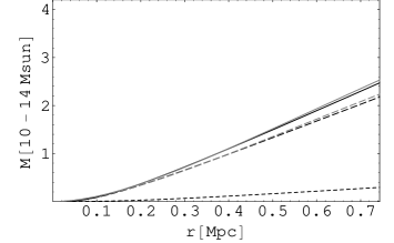
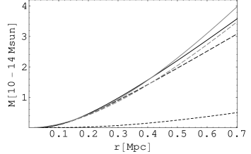
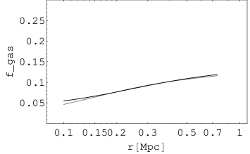
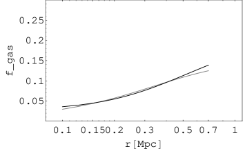
Figure 2: (Top) Mass profiles for the RIS model and the NFW profile for A496 (left) and Coma (right). The thick short-dashed line is the mass $M_{X}(r)$ associated with the ICM; the thick long-dashed-line (RIS model) and the thin long-dashed line (NFW) are the mass $M_{DM}(r)$ associated with the dark matter; the thick solid line (RIS model) and the thin solid line (NFW) are the total mass profile $M_{tot}(r)$. On the vertical axis the mass is expressed in units of $10^{14}\ {\rm{M}_{\odot}}$. (Bottom) Gas fraction $f_{gas}(r)$ for the RIS model (thick line) and the NFW profile (thin line) for A496 (left) and Coma (right). The figure is based on $h=0.5$.

In order to better appreciate the relative concentration of dark and visible matter for the models identified in Tables 2 and 3, we may refer to the integrated mass profiles introduced in Sect. 2 (see Eqs. (3), (4)). The various profiles are illustrated in Fig. 2. Tables 4 and 5 summarize some characteristics of the best-fit models.

Table 4: Mass associated with the ICM ($M_{X}$), mass associated with the dark matter ($M_{DM}$), total mass ($M_{tot}$), and gas fraction ($f_{gas}$) evaluated at $r_{out}=743\ \rm{kpc}$, for the best-fit RIS model and NFW profile for A496 ($h=0.5$).

Model	$M_{X}(r_{out})$	$M_{DM}(r_{out})$	$M_{tot}(r_{out})$	$f_{gas}(r_{out})$
	($10^{14}\ {\rm{M}_{\odot}}$)	($10^{14}\ {\rm{M}_{\odot}}$)	($10^{14}\ {\rm{M}_{\odot}}$)
RIS	0.294	2.18	2.47	0.119
NFW	0.294	2.24	2.53	0.116

Table 5: Mass associated with the ICM ($M_{X}$), mass associated with the dark matter ($M_{DM}$), total mass ($M_{tot}$), and gas fraction ($f_{gas}$) evaluated at $r_{out}=702\ \rm{kpc}$, for the best-fit RIS model and NFW profile for Coma ($h=0.5$).

Model	$M_{X}(r_{out})$	$M_{DM}(r_{out})$	$M_{tot}(r_{out})$	$f_{gas}(r_{out})$
	($10^{14}\ {\rm{M}_{\odot}}$)	($10^{14}\ {\rm{M}_{\odot}}$)	($10^{14}\ {\rm{M}_{\odot}}$)
RIS	0.498	3.09	3.58	0.139
NFW	0.498	3.49	3.98	0.125

Figure 2 shows that, in each cluster, the gas fraction increases with the distance from the center, i.e. the dark matter is more concentrated than the visible matter. Note that this statement holds for two very different models of the density distribution of dark matter, which turn out to exhibit only modest quantitative differences in relation to the issues addressed in this paper.

As noted at the end of Sect. 1, in this paper the analysis has been carried out under the assumption of a rather low Hubble constant, with $h=0.5$. It is easy to convert the relevant quantitative estimates to those appropriate for a different value of $h$ by recalling (e.g., see [2]) that lengths (such as $r_{X}$ of Table 1) scale as $h^{-1}$, gas densities ($n_{0}$ and ${\rho_{X}}^{(0)}$ of Table 1) as $h^{1/2}$, the integrated ICM mass (see $M_{X}$ in Tables 4 and 5) as $h^{-5/2}$, the total binding mass (see $M_{tot}$ in Tables 4 and 5) as $h^{-1}$, and finally the gas fraction (see $f_{gas}$ in Tables 4 and 5) as $h^{-3/2}$. Of course $\lambda$ is independent of $h$.

For example, for $h=0.7$ we would have for Coma $r_{out}=\rm{501\ kpc}$ (instead of 702 kpc) and a cut in the central regions $r_{cut}=\rm{71\ kpc}$ (instead of 100 kpc); the length scales for the best-fit RIS model and NFW profile along with the integrated masses associated with them are reported in Table 6.

Table 6: Length scales for the ICM ($r_{X}$) and the dark matter ($r_{DM}$), mass associated with the ICM ($M_{X}$), mass associated with the dark matter ($M_{DM}$), total mass ($M_{tot}$), and gas fraction ($f_{gas}$) evaluated at $r_{out}=501\ \rm{kpc}$, for the best-fit RIS model and NFW profile for Coma, for a Hubble constant corresponding to $h=0.7$.

Model	$r_{X}$	$r_{DM}$	$M_{X}(r_{out})$	$M_{DM}(r_{out})$	$M_{tot}(r_{out})$	$f_{gas}(r_{out})$
	(Mpc)	(Mpc)	($10^{14}\ {\rm{M}_{\odot}}$)	($10^{14}\ {\rm{M}_{\odot}}$)	($10^{14}\ {\rm{M}_{\odot}}$)
RIS	0.293	0.088	0.215	2.35	2.56	0.084
NFW	0.293	0.955	0.215	2.63	2.84	0.076

5 The role of the galaxies

The relatively low values of $f_{gas}$ recorded in Table 6 suggest that we should check the role of the galaxies in the mass budget of a cluster. In fact, so far we have neglected the explicit contribution of galaxies or, rather, absorbed their contribution into the dark matter component of the mass distribution.

We focus on the case of Coma. In their study based on $h=0.7$, Łokas & Mamon [21] fit the three-dimensional luminosity density profile of the galaxies in Coma with a NFW profile and then obtain the mass distribution of the galaxies by multiplying by a mean mass-to-light ratio (blue band) appropriate for the morphological population of the cluster, $\Upsilon_{G}=6.43\ \rm{M_{\odot}/L_{\odot}}$. They find a length scale for the galaxy distribution $r_{s}=0.411\ \rm{Mpc}$. For a direct comparison with the simple modeling considered in our paper, we have referred to a RIS profile

$$\rho_{G}(x)={\rho_{G}}^{(0)}\left[1+\left(\frac{x}{\lambda_{G}}\right)^{2}\right]^{-1}\ ,$$ (10)

where $\lambda_{G}=r_{G}/r_{X}$, being $r_{G}$ the length scale of the galaxies. We have found that for $r_{G}=0.071\ \rm{Mpc}$, corresponding to $\lambda_{G}=0.24$, and actually equal to $r_{cut}$, such profile gives a similarly adequate representation of the galaxy density distribution in the cluster. These latter values should be compared with the dark matter distribution length scale and concentration parameter we found for the RIS profile (see Tables 6 and 3), $r_{DM}=0.088\ \rm{Mpc}$ and $\lambda=0.30$ respectively. This shows that, in the Coma cluster, galaxies are somewhat more concentrated with respect to dark matter and confirms the argument that led to the choice of the cut in the inner regions, as discussed in Sect. 3. On the other hand, we see that the difference between $\lambda_{G}=0.24$ and $\lambda=0.30$ is rather small, so that, a posteriori, our choice of combining together, into a unique density profile $\rho_{DM}(r)$, dark matter and the smaller contribution of matter associated with galaxies was indeed very reasonable.

In order to quantify the effects of neglecting the galaxy contribution, in Table 7 we report, for $r_{cut}$ and $r_{out}$, the mass of the galaxies and the actual mass of dark matter (i.e. the difference between the mass of what we have called dark matter so far and the mass of the galactic component), in addition to the mass of the ICM and the total mass, together with the gas fraction and the galactic fraction

$$f_{G}(r)=\frac{M_{G}(r)}{M_{tot}(r)}\ ;$$ (11)

here $M_{G}(r)$ is the cumulative mass obtained by integrating Eq. (10).

Table 7: Mass associated with the galaxies ($M_{G}$), mass associated with the ICM ($M_{X}$), actual mass associated with the dark matter ($M_{DM}^{actual}$), total mass ($M_{tot}$), galactic fraction ($f_{G}$), and gas fraction ($f_{gas}$) evaluated at $r_{cut}=71\ \rm{kpc}$ and $r_{out}=501\ \rm{kpc}$, for the best-fit RIS model for Coma, for a Hubble constant corresponding to $h=0.7$.

Radius	$M_{G}(r)$	$M_{X}(r)$	$M_{DM}^{actual}(r)$	$M_{tot}(r)$	$f_{G}(r)$	$f_{gas}(r)$
(Mpc)	($10^{14}\ {\rm{M}_{\odot}}$)	($10^{14}\ {\rm{M}_{\odot}}$)	($10^{14}\ {\rm{M}_{\odot}}$)	($10^{14}{\rm{M}_{\odot}}$)
0.071	0.00208	0.00147	0.0646	0.0682	0.030	0.022
0.501	0.0545	0.215	2.29	2.56	0.021	0.084

We note from Table 7 that the contribution by the galaxies to the total mass is at most of 3% at every radius outside $r_{cut}$; we also see (cf. Fig. 3) that the fraction of the sum $f_{G}(r)+f_{gas}(r)$ increases with radius, confirming again that dark matter is concentrated with respect to visible matter, even when we include the contribution of the mass associated with galaxies.

Finally, we have tested the effect of increasing the value of the mass-to-light ratio associated with galaxies, above the value adopted by Łokas & Mamon [21], as would be appropriate to do if galaxies were associated with increasingly dominant dark matter halos. The combined value $f_{G}(r)+f_{gas}(r)$ remains definitely a monotonic increasing function of radius even when we double the galaxy mass-to-light ratio. Only at $\Upsilon_{G}\approx 30\ \rm{M_{\odot}/L_{\odot}}$ does the trend start to reverse.

6 Conclusions

In this work we have studied the relative distribution of the ICM mass with respect to the total mass for two galaxy clusters. These clusters (A496 and Coma) were chosen as representative of the classes of cool-core and non-cool-core clusters respectively.

The main point of the paper is that some interesting conclusions can be drawn by means of an extremely simple analysis. They are the following:

1. We find that dark matter is concentrated with respect to visible matter. This result confirms previous investigations (see Markevitch et al. [20]), but has been obtained here without imposing a global equation of state for the ICM or a cosmologically suggested density profile for the dark matter distribution. Therefore, our simple result contributes significant confidence in the robustness of this general conclusion.

2. On the large scale explored by the data used and the dynamical model adopted, the RIS model and the NFW profile are substantially equivalent and we cannot really tell whether a cusp of dark matter is present or absent. This conclusion basically confirms a natural expectation.

3. The two clusters studied here, although very different from the morphological point of view, exhibit a similar behaviour with respect to the issue addressed in this paper (see also Ettori et al. [3]).

4. For the currently favored value of the Hubble constant, $h=0.7$, the relative contribution of galaxies to the mass budget requires a detailed check, because, with respect to the case $h=0.5$, it is less obvious that on the scale of $0.5~{}\rm{Mpc}$ the visible mass be dominated by the intracluster medium. A quantitative test for the Coma cluster has shown that indeed the contribution of galaxies is dominant only in the innermost regions excluded by our cut to the data, inside $0.1~{}\rm{Mpc}$. The conclusion that dark matter is more concentrated than visible matter remains valid even when the contribution of the galactic component to the visible mass is considered explicitly.

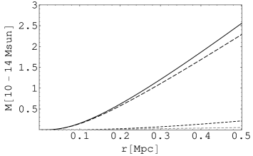
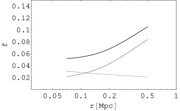
Figure 3: (Left) Mass profiles for the RIS model for Coma. The thin short-dashed line is the mass $M_{G}(r)$ associated with the galaxies; the thick short-dashed line is the mass $M_{X}(r)$ associated with the ICM; the thick long-dashed-line is the actual mass $M_{DM}^{actual}(r)$ associated with the dark matter; the thick solid line is the total mass profile $M_{tot}(r)$. On the vertical axis the mass is expressed in units of $10^{14}\ {\rm{M}_{\odot}}$. (Right) Galaxy fraction $f_{G}(r)$ (thin dashed line), gas fraction $f_{gas}(r)$ (thin solid line), and visible mass fraction $f_{G}(r)+f_{gas}(r)$ (thick solid line) for the same RIS model for Coma. The figure is based on a Hubble constant corresponding to $h=0.7$.