Simultaneous numerical simulation of direct and inverse cascades in wave turbulence.

Abstract

Results of direct numerical simulation of isotropic turbulence of surface gravity waves in the framework of Hamiltonian equations are presented. For the first time simultaneous formation of both direct and inverse cascades was observed in the framework of primordial dynamical equations. At the same time, strong long waves background was developed. It was shown, that obtained Kolmogorov spectra are very sensitive to the presence of this condensate. Such situation has to be typical for experimental wave tanks, flumes, and small lakes.

–Introduction – In this year we have a 50th anniversary of the famous work by Phillips Phillips1958 which was, probably, the first attempt to give an explanation for power-like spectra of surface gravity waves observed in numerous experiments. In recent works Kuznetsov2004 ; NZ2008 the physical explanation given by Phillips was corrected. During less than ten years after that the statistical theory of surface waves was founded: Hasselmann derived kinetic equation for waves Hasselmann1962 , Zakharov created theory of wave (or weak) turbulence ZakharovPhD ; ZFL1992 , which describes solutions of this equation. Stationary Kolmogorov solutions of the kinetic equation corresponding to flux of energy from large to small scales (direct cascade) and flux of wave action (waves “numbers”) from small to large scales (inverse cascade) were found ZF1967 ; ZFL1992 . This opened a way to creation of the effective tool for waves forecasting. The conjectures under which the theory of weak turbulence was derived includes Gaussian statistics for waves field and resonant interactions prevalence ZFL1992 . They are subject for confirmation. Modern numerical methods allow to perform wave field modeling in the framework of kinetic equation faster than real processes in nature. At the same time, it is impossible to create waves forecasting model based on direct numerical simulation of dynamic equations. Even more, we do not need to know velocity and elevation at every point of the surface. Statistics, especially mean wave hight and speed, this is what really matters for estimation of operational conditions of oil platforms and cargo ships. And this is exactly the subject of theory of weak turbulence. In means that the problem of confirmation and correction of the waves turbulence is of great practical importance.

Experiments in the open sea and on the Great Lakes gave temporal and space spectra consistent with the theory Toba1973 ; Donelan1985 ; Hwang2000 . A comprehensive review of experiments and comparison with the theory of the weak turbulence can be found in BPRZ2005 ; Zakharov2005 ; BBRZ2007 . Most of these experiments were performed with wind pumping, broad in spectrum. Narrow in spectrum pumping can be realized in wave tanks or flumes. Results obtained on such state of the art devices frequently contradict with predictions of the theory of wave turbulence. For example, in the recent experiments FFL2007 ; Lukaschuk2007 observed spectra were changing slope with variation of steepness and pumping force.

May be the most promising way to check conjectures of the waves turbulence theory is a numerical experiment. In the case of direct numerical simulation we have the highest possible control on the parameters of experiments and all information about the wave field. At the same time all this data is given at the cost of the enormous computational complexity. Fast growth of computational power and development of computational algorithms allowed direct numerical simulation of the surface gravity waves, starting from the simulations of the swell evolution Tanaka2001 ; Onorato2002 ; Yokoyama2004 ; ZKPD2005 ; ZKPR2007 ; KPRZ2008 to the isotropic turbulence simulation DKZ2003grav ; DKZ2004 ; LNP2006 ; AS2006 . There is a hope, that this approach together with confirmation of conjectures of the weak turbulent theory will allow us to explain phenomena observed in experimental wave tanks.

At the same time, theory of the wave turbulence is still under development. To close the circle the recent paper by Newell and Zakharov NZ2008 gave second life to the Phillips spectrum, although from completely different point of view: Phillips spectrum considered to be a solution which give a balance of transfer of energy due to nonlinear waves interaction transfer of energy and transfer due to intermittent events, like wave breaking and white capping.

This Letter was inspired by several recent papers. In the first one AS2006 numerical simulation of the isotropic turbulence with observed formation of inverse cascade was performed in the framework of Zakharov equations ZFL1992 . A little bit later a group of authors Chertkov2007 during simulation of 2D hydrodynamics observed formation of large scale structure due to Kraichnan’s inverse cascade and explored its influence on the system. Approximately at the same time state of the art surface waves wave flume experiment was performed Lukaschuk2007 . Observed spectra differed from the theory wave turbulence. Author performed a direct numerical simulation of isotropic turbulence of surface gravity waves in the framework of Hamiltonian equations. The isotropic turbulence is a classical setup for turbulence investigation. In nature such such wave field is usually observed in the regions with large amount of floating broken ice. For the first time the formation of both direct and inverse cascades was observed in the framework of primordial dynamical equations. At the same time, strong long waves background was developed. This phenomenon of “condensation” of waves (following analogy with Bose-Einstein condensation in condensed matter physics) was predicted by the theory of weak turbulence. It was shown, that obtained Kolmogorov spectra are very sensitive to the presence of the condensate. Such situation have to be typical for experimental wave tanks, flumes and small lakes. Obtained results can be considered as the first observation of generalized Phillips spectra, introduced in NZ2008 and explain some deviations from the waves turbulence theory in recent wave tank experiments.

–Theoretical background – We consider a potential flow of ideal incompressible fluid. System is described in terms of weakly nonlinear equations ZFL1992 ; DKZ2004 for surface elevation $\eta(\vec{r},t)$ and velocity potential at the surface $\psi(\vec{r},t)$ ($\vec{r}=\overrightarrow{(x,y)}$)

$$\dot{\eta}=\hat{k}\psi-(\nabla(\eta\nabla\psi))-\hat{k}[\eta\hat{k}\psi]+$$

$$+\hat{k}(\eta\hat{k}[\eta\hat{k}\psi])+\frac{1}{2}\Delta[\eta^{2}\hat{k}\psi]+\frac{1}{2}\hat{k}[\eta^{2}\Delta\psi]+\widehat{F}^{-1}[\gamma_{k}\eta_{k}],$$

$$\dot{\psi}=-g\eta-\frac{1}{2}\left[(\nabla\psi)^{2}-(\hat{k}\psi)^{2}\right]-$$ (1)

$$-[\hat{k}\psi]\hat{k}[\eta\hat{k}\psi]-[\eta\hat{k}\psi]\Delta\psi+\widehat{F}^{-1}[\gamma_{k}\psi_{k}]+P_{\vec{r}}.$$

Here dot means time-derivative, $\Delta$ — Laplace operator, $\hat{k}$ is a linear integral operator $\left(\hat{k}=\sqrt{-\Delta}\right)$, $\widehat{F}^{-1}$ is an inverse Fourier transform, $\gamma_{k}$ is a dissipation rate (according to recent work DDZ2008 it has to be included in both equations), which corresponds to viscosity on small scales and, if needed, ”artificial” damping on large scales. $P_{\vec{r}}$ is the driving term which simulates pumping on large scales (for example, due to wind). In the $k$-space supports of $\gamma_{k}$ and $P_{\vec{k}}$ are separated by the inertial interval, where the Kolmogorov-type solution can be recognized. These equations were derived as a results of Hamiltonian expansion in terms of $\hat{k}\eta$. From physical point of view $\hat{k}$-operator is close to derivative, so we expand in powers of slope of the surface. In most of experimental observations average slope of the open sea surface $\mu$ is of the order of $0.1$, so such expansion is very reasonable.

In the case of statistical description of the wave field, Hasselmann kinetic equation Hasselmann1962 for the distribution of the wave action $n(k,t)=\langle|a_{\vec{k}}(t)|^{2}\rangle$ is used. Here

$$a_{\vec{k}}=\sqrt{\frac{\omega_{k}}{2k}}\eta_{\vec{k}}+\mathrm{i}\sqrt{\frac{k}{2\omega_{k}}}\psi_{\vec{k}},$$ (2)

are complex normal variables. For gravity waves $\omega_{k}=\sqrt{gk}$.

From the theory of weak turbulence ZFL1992 , besides equipartions (Rayleigh-Jeans) spectrum, we know two stationary solutions ZF1967 ; ZakharovPhD of the kinetic equation in the case of four-waves interaction:

$$n_{k}^{(1)}=C_{1}P^{1/3}k^{-\frac{2\beta}{3}-d},\;\;n_{k}^{(2)}=C_{2}Q^{1/3}k^{-\frac{2\beta-\alpha}{3}-d}.$$ (3)

For surface gravity waves, a coefficient of homogeneity of nonlinear interaction matrix element $\beta=3$, the power of dispersion law $\alpha=1/2$, and the dimension of the surface $d=2$. As a result we get

$$n_{k}^{(1)}=C_{1}P^{1/3}k^{-4},\;\;\;n_{k}^{(2)}=C_{2}Q^{1/3}k^{-23/6}.$$ (4)

The first solution $n_{k}^{(1)}$ describes direct cascade of energy from large pumping to small dissipative scales. The second solution $n_{k}^{(2)}$ describes inverse cascade of action (or “number” of waves) from small pumping to larger scales.

–Numerical simulation – We simulated primordial dynamical equations (1) in a periodic spatial domain $2\pi\times 2\pi$. Main part of the simulations was performed on a grid consisting of $1024\times 1024$ knots. Also we performed long time simulation on the grid $256\times 256$. The used numerical code was verified in DKZ2003cap ; DKZ2003grav ; DKZ2004 ; ZKPD2005 ; ZKPR2007 ; KPRZ2008 . Gravity acceleration was $g=1$. Pseudo-viscous damping coefficient had the following form

$$\gamma_{k}=\cases{0,k\leq k_{d},\cr-\gamma_{0}(k-k_{d})^{2},k>k_{d},\cr}$$ (5)

where $k_{d}=256$ and $\gamma_{0,1024}=2.7\times 10^{4}$ for the grid $1024\times 1024$ and $k_{d}=64$ and $\gamma_{0,256}=2.4\times 10^{2}$ for the smaller grid $256\times 256$. Pumping was an isotropic driving force narrow in wavenumbers space with random phase:

$$P_{\vec{k}}=f_{k}\mathrm{e}^{\mathrm{i}R_{\vec{k}}(t)},f_{k}=\cases{4F_{0}\frac{(k-k_{p1})(k_{p2}-k)}{(k_{p2}-k_{p1})^{2}},\cr 0-\mathrm{if}\;k<k_{p1}\;\mathrm{or}\;k>k_{p2};\cr}$$ (6)

here $k_{p1}=28,\;k_{p2}=32$ and $F_{0}=1.5\times 10^{-5}$; $R_{\vec{k}}(t)$ was uniformly distributed random number in the interval $(0,2\pi]$ for each $\vec{k}$ and $t$. Initial condition was low amplitude noise in all harmonics. Time steps were $\Delta t_{1024}=6.7\times 10^{-4}$ and $\Delta t_{256}=5.0\times 10^{-3}$. We used Fourier series in the following form:

$$\eta_{\vec{k}}=\widehat{F}[\eta_{\vec{r}}]=\frac{1}{(2\pi)^{2}}\int\limits_{0}^{2\pi}\int\limits_{0}^{2\pi}\eta_{\vec{r}}\mathrm{e}^{\mathrm{i}\vec{k}\vec{r}}\mathrm{d}^{2}r,$$

$$\eta_{\vec{r}}=\widehat{F}^{-1}[\eta_{\vec{r}}]=\sum\limits_{-N_{x}/2}^{N_{x}/2}\sum\limits_{-N_{y}/2}^{N_{y}/2}\eta_{\vec{k}}\mathrm{e}^{-\mathrm{i}\vec{k}\vec{r}},$$

here $N_{x}$, $N_{y}$ — are number of Fourier modes in $x$ and $y$ directions.

As a results of simulation we observed formation of both direct and inverse cascades (Fig. 1, solid line), although exponents of power-like spectra were different from weak turbulent solutions (4). What is important, development of inverse cascade spectrum was arrested by discreteness of wavenumbers grid in agreement with DKZ2003cap ; ZKPD2005 ; Nazarenko2006 . After that large scale condensate started to form. As one can see, value of wave action $|a_{k}|^{2}$ at the condensate region is more than order of magnitude larger than for closest harmonic of inverse cascade. Dynamics of large scales became extremely slow after this point. We managed to achieve downshift of condensate peak for one step of wavenumbers grid during long time simulation on a small grid $256\times 256$ (Fig. 1, line with long dashes). As one can see we observed elongation of inverse cascade interval without significant change of the slope. Unfortunately, inertial interval for inverse cascade is too short to exclude possible influence of pumping and condensate.

Figure 1: Spectra $<|a_{k}|^{2}>$. With condensate on the $1024\times 1024$ grid (solid); on the $256\times 256$ grid with more developed condensate (long dashes); without condensate on the $1024\times 1024$ grid (short dashes).

We can try to estimate exponent by compensation of the spectra in a double logarithmic scale (Fig. 2). The observed spectrum $\sim k^{-3.5}$ is close to weak turbulent solution (3). Slightly lower exponent could be explained by weakening of resonant nonlinear interactions on the rough wavenumbers grid, which effectively decreases the homogeneity coefficient $\beta$ in the expression (3).

Figure 2: Compensated inverse cascade spectra $C\langle|a_{k}|^{2}\rangle k^{s}$.

For direct cascade spectra we also used compensation in double logarithmic scale. Results are present in Fig. 3 (left). Formally, in this case we have quite long inertial interval $32<k<256$, but in reality damping has an influence on the spectrum approximately up to $k\simeq 180$. Still in this case we have more than half of a decade. Theory of weak turbulence gives us dependence $\sim k^{-4}$ (3), known as Kolmogorov-Zakharov spectrum. Nevertheless, one can see that we observe $k^{-9/2}$, known as Phillips Phillips1958 ; NZ2008 spectrum. So we need to understand, what is the reason of different spectrum slope? What changes weak turbulent theory in this case?

Figure 3: Compensated direct cascade spectra $C\langle|a_{k}|^{2}\rangle k^{s}$ with (left) and without (right) condensate.

To answer these questions let us compare our situation with previous works on decaying Onorato2002 ; ZKPR2007 ; KPRZ2008 or isotropic DKZ2003grav ; DKZ2004 ; LNP2006 turbulence. Immediately we have an answer: condensate and inverse cascade spectrum! The inverse cascade’s part of the spectrum is described by the theory of weak turbulence, so let us concentrate on the strong long ($k\simeq 5$) waves’ influence on much shorter waves ($32<k<180$), corresponding to direct cascade. We suppressed condensate by including “artificial” dissipation on large scales ($k<10$). Resulting spectrum is given in Fig. 1 (line with short dashes). The best wave to see the difference in characteristic waves’ scale is to have a look at the surface with and without condensate (Fig. Surface).

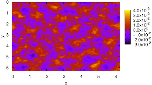
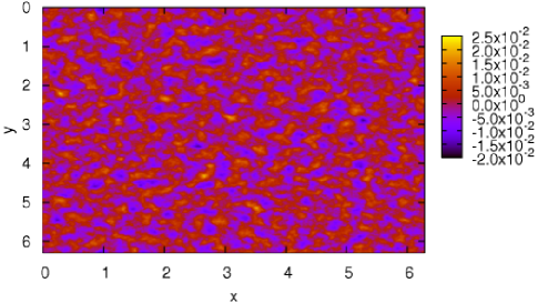
Figure 4: Surface of the fluid $\eta(\vec{r})$ with (left) and without (right) condensate.

Compensated spectrum for direct cascade is given in Fig. 3 (right). As one can see exponent of the spectrum changed and is now closer to the results of weak turbulent theory. The light difference may be a result of the influence of the left edge of inverse cascade, which can play a role of condensate for short scales corresponding to the direct cascade.

Qualitative explanation of the condensate’s influence on the short waves could be the following: let us consider propagating stationary wave with some given slope of the front, much longer wave can be treated as a presence of a strong background flow. If the direction of the flow is opposite to direction of wave propagation the slope of the wave’s front will increase. This is what we see in our simulations. Average steepness $\mu=\sqrt{<|\vec{\nabla}\eta|^{2}>}$ has changed: with condensate $\mu_{c}\simeq 0.14$, without condensate $\mu_{nc}\simeq 0.12$. More detailed picture is given by probability distribution functions (PDFs) for surface slopes (Fig. 5-6). Although maximums of distributions are well described by Gaussian distribution (which is one of the assumption of the weak turbulence theory), we have significant non-Gaussian tails and, what is more important, widths of PDFs are different. It means, that in the presence of condensate steeper waves are more probable.

Figure 5: PDFs of $\vec{\nabla}_{x}\eta$ with (left) and without (right) condensate.

Figure 6: PDFs of $\vec{\nabla}_{y}\eta$ with (solid) and without (dashed) condensate.

Surface elevation PDFs, given in Fig. 7 in both cases are in a good agreement with Tayfun distribution Tayfun1980 , which is the first nonlinear correction to Gaussian distribution.

Figure 7: PDFs of surface elevation $\eta(\vec{r})$ with (left) and without (right) condensate.

In nature it will result in stronger “whitecapping”: formation of white foam cap on the crest of the wave causing additional transport of energy to the small dissipative scale. In the framework of our model such micro-wavebreaking is impossible. Dissipation in the system prevents formation of strong spectrum tails corresponding to formation of discontinuities on the surface. Nevertheless, the mechanism is quite similar: higher steepness means stronger nonlinearity in our system. In this case for harmonics close enough to the dissipation region generation of second and third harmonics acts as fast and effective additional process of energy transport to the dissipative scales. Processes, corresponding to multiple harmonics generation are non-resonant and they are neglected in the theory of wave turbulence. Also it explains why in the experiment in the framework of Zakharov’s equations AS2006 spectra were close to weak turbulent. Zakharov’s equations take into account only resonant interactions and do not describe multiple harmonics generation. We can see, that catastrophic events, like formation of sharp crests, which cannot be described in the statistical framework of kinetic equation, can significantly affect physics in the system. The waves kinetic equation can be augmented by additional dissipation term to simulate this dissipation. As it was shown in recent open field BBY2000 and numerical ZKPR2007 experiments, whitecapping dissipation is a phenomenon similar to a second order phase transition, so even such a moderate change of the average steepness as we observed can cause significant altering of the energy transfer mechanism. Our results in the presence of condensate can be considered as the first proof of a conjecture NZ2008 , that Phillips spectrum corresponds to a physical picture when a balance between nonlinear transport terms and intermittent dissipation takes place.

–Conclusion – In this Letter author presented results of the first direct numerical simulation of the direct cascade in the presence of inverse cascade and condensate. The importance of condensate as a factor, which increases average steepness and stimulates additional intermittant dissipation, is demonstrated. Qualitative explanation of observed spectra is given. The quantitative explanation is a subject of further investigations. Still there is no comprehensive theory of whitecapping, which includes analysis of fully nonlinear equations. One can use presented results for explanation of observed differences in the spectra in open see and water tanks experiments.

- (1) O. M. Phillips, J. Fluid Mech. 4, 426 (1958).
- (2) E. A. Kuznetsov, JETP Letters 80, 83 (2004).
- (3) A. C. Newell and V. E. Zakharov, Phys. Lett. A, article in press (2008).
- (4) K. Hasselmann, J. Fluid Mech. 12, 48, 1 (1962).
- (5) V. E. Zakharov, PhD thesis, Budker Institute for Nuclear Physics, Novosibirsk, USSR (1967).
- (6) V. E. Zakharov, G. Falkovich, and V. S. Lvov, Kolmogorov Spectra of Turbulence I (Springer-Verlag, Berlin, 1992).
- (7) V. E. Zakharov and N. N. Filonenko, Sov. Phys. Dokl. 11, 881 (1967).
- (8) Y. Toba, J. Oceanogr. Soc. Japan 29, 209 (1973).
- (9) M. A. Donelan, J. Hamilton, and W. H. Hui, Phil. Trans. R. Soc. London A315, 509 (1985).
- (10) P. A. Hwang at al., J. Phys. Oceanogr. 30, 2753 (2000).
- (11) S. I. Badulin et al., Nonlin. Proc. Geophys. 12, 891 (2005).
- (12) V. E. Zakharov, Nonlin. Proc. Geophys. 12, 1011 (2005).
- (13) S. I. Badulin et al., Journ. Fluid. Mech. 591, 339 (2007).
- (14) E. Falcon, S. Fauve, and C. Laroche, Phys. Rev. Lett. 98, 154501 (2007).
- (15) P. Denissenko, S. Lukaschuk, and S. Nazarenko, Phys. Rev. Lett. 99, 014501 (2007).
- (16) M. Tanaka, J. Fluid Mech. 444, 199 (2001).
- (17) M. Onorato at al., Phys. Rev. Lett. 89, 14, 144501 (2002).
- (18) N. Yokoyama, J. Fluid Mech. 501, 169 (2004).
- (19) V. E. Zakharov et al., JETP Lett. 82, 8, 487 (2005). arXiv:physics/0508155.
- (20) V. E. Zakharov et al., Phys. Rev. Lett. 99, 164501 (2007). arXiv:0705.2838
- (21) A. O. Korotkevich et al., Eur. J. Mech. B/Fluids, in press (2008). arXiv:physics/0702145
- (22) A. I. Dyachenko, A. O. Korotkevich, and V. E. Zakharov, JETP Lett. 77, 10, 546 (2003). arXiv:physics/0308101
- (23) A. I. Dyachenko, A. O. Korotkevich, and V. E. Zakharov, Phys. Rev. Lett. 92, 13, 134501 (2004). arXiv:physics/0308099.
- (24) Yu. Lvov, S. V. Nazarenko, and B. Pokorni, Physica D 218, 1, 24 (2006). arXiv:math-ph/0507054.
- (25) S. Y. Annenkov and V. I. Shrira, Phys. Rev. Lett. 96, 204501 (2006).
- (26) M. Chertkov et al., Phys. Rev. Lett. 99, 084501 (2007).
- (27) F. Dias, A. I. Dyachenko, and V. E. Zakharov, Phys. Lett. A, 372, 8, 1297 (2008). arXiv:0704.3352
- (28) A. I. Dyachenko, A. O. Korotkevich, and V. E. Zakharov, JETP Lett. 77, 9, 477 (2003). arXiv:physics/0308100.
- (29) S. V. Nazarenko, J. Stat. Mech. L02002 (2006). arXiv:nlin/0510054.
- (30) A. Tayfun, Journ. of Geophys. Res., 85, 1548 (1980).
- (31) M. L. Banner, A. V. Babanin, I. R. Young, J. Phys. Oceanogr. 30, 3145 (2000).
- (32) http://fftw.org, M. Frigo and S. G. Johnson, Proc. IEEE 93, 2, 216 (2005).