X-ray Dust Scattering at Small Angles: The Complete Halo around GX13+1

Abstract

The exquisite angular resolution available with Chandra should allow precision measurements of faint diffuse emission surrounding bright sources, such as the X-ray scattering halos created by interstellar dust. However, the ACIS CCDs suffer from pileup when observing bright sources, and this creates difficulties when trying to extract the scattered halo near the source. The initial study of the X-ray halo around GX13+1 using only the ACIS-I detector done by Smith, Edgar & Shafer (2002) suffered from a lack of sensitivity within $50^{\prime\prime}$ of the source, limiting what conclusions could be drawn.

To address this problem, observations of GX13+1 were obtained with the Chandra HRC-I and simultaneously with the RXTE PCA. Combined with the existing ACIS-I data, this allowed measurements of the X-ray halo between 2-1000”. After considering a range of dust models, each assumed to be smoothly distributed with or without a dense cloud along the line of sight, the results show that there is no evidence in this data for a dense cloud near the source, as suggested by Xiang et al. (2005). Finally, although no model leads to formally acceptable results, the Weingartner & Draine (2001) and nearly all of the composite grain models from Zubko, Dwek & Arendt (2004) give poor fits.

1. Introduction

Practically every band of the electromagnetic spectrum affects or is affected by interstellar (IS) dust grains. In the IR, PAHs emit lines and small grains emit continuum radiation; in the UV/optical, small grains both extinct and scatter light. In X-rays, large dust grains ($>0.1\mu$m) scatter X-rays, creating halos around point sources. The classic paper by Mathis, Rumpl & Nordsieck (1977, MRN77) used the observed optical extinction to determine the size distribution of dust grains between 0.005-0.25$\mu$m. Newer models, such as Weingartner & Draine (2001, WD01), have extended the modeling to include polycyclic aromatic hydrocarbons (PAHs) to match the observed IR emission as well as other constraints on grain abundances. Recently, Zubko, Dwek & Arendt (2004, ZDA04) found that a wide range of dust compositions and size distributions could fit the existing data, and suggested that new observational constraints from X-ray halos are needed to select amongst these models.

X-ray dust scattering halos are created by the small-angle scattering of X-rays as they pass through dust grains. When an incoming X-ray interacts with the electrons in a grain large compared to the X-ray wavelength, the resulting Rayleigh scattering adds coherently in the forward direction leading to small-angle scattering; see van de Hulst (1957) and Mathis & Lee (1991) for details, and Draine (2003) for a comprehensive review. More generally, the scattering problem can be posed as that of a wave interacting with a sphere, in which case the Mie solution applies (e.g. Smith & Dwek, 1998). In either approach, the scattering depends largely on the grain size distribution, with lesser dependencies on the grain composition and position along the line of sight.

Observations of X-ray scattered halos have just begun to significantly impact dust models. Smith, Edgar & Shafer (2002, (SES02)) described Chandra observations of GX13+1 with the ACIS-I detector and showed that dust grains do not have large ($\gtrsim 0.8$) vacuum fractions considered by Mathis & Whiffen (1989). SES02 also found that the extremely large grains found by Ulysses in the solar neighborhood (Landgraf et al., 2000; Witt, Smith & Dwek, 2001) do not seem to be common throughout the Galaxy. Despite these successes, SES02 could not distinguish between the MRN77 and WD01 models. This was in part due to calibration uncertainties as well as inherent limitations of the data. Despite Chandra’s excellent angular resolution, ACIS-I observations of GX13+1 could not measure the halo within $50^{\prime\prime}$, due to massive pileup in the ACIS-I detectors. Draine (2003) and Xiang et al. (2005) have both noted that this result is therefore insensitive to dust near the source, as scattering from dust within the last 25% of the distance would lead to features primarily within the excluded $50^{\prime\prime}$. To address this shortcoming, I obtained a short Chandra HRC-I observation of GX13+1. The multichannel plate design of the HRC-I is far less sensitive to large count rates, which allows GX13+1’s radial profile to be measured to within 2” of the source, far closer than previously possible.

2. Observations

GX13+1 was observed simultaneously with the Chandra HRC-I and RXTE Proportional Counter Array (PCA) on February 8, 2005 for 9.1 ksec (ObsID 6093) and 6.2 ksec (P90173), respectively. CIAO v3.3 software was used to process the Chandra data, which showed significant background flares in addition to the flux from the bright source. Standard processing was used for the RXTE data.

2.1. Selecting Good Events

The full-field lightcurve included significant periods when the count rate approached the 184 cts s^-1 telemetry limit. The expected HRC-I background rate for the full field is $\sim 50$ cts s^-1 (Chandra X-ray Center, 2006). Despite the brightness of the source, the telemetry saturation was in fact primarily due to the particle background. After excluding a 2’ radius circle around GX13+1, the average count rate was $<50$ cts s^-1, but with excursions above 100 cts s^-1 where telemetry saturation would affect the data. To eliminate this problem only time periods where the total counts in the field (i.e, $>2^{\prime}$ from GX13+1) were $<45$ cts s^-1 were included. Although this reduced the total good time to 3.58 ksec, $\sim 200,000$ counts were detected within $2^{\prime}$ of GX13+1 for a source count rate of 54.8 cts s^-1. All of these effects can be seen in Figure 1, which shows the total HRC-I count rate, the HRC-I count rate within $2^{\prime}$ of GX13+1, and the RXTE PCA lightcurve (between 2-9 keV) during the observation. Within $2^{\prime\prime}$ of GX13+1 the count rate during these 3.58 ksec was 42.7 cts s^-1. According to §4.2.3.1 of the Chandra Proposer’s Observatory Guide, the encircled energy within $2^{\prime\prime}$ is $\approx 90$%, rising to $\approx 95\%$ within $10^{\prime\prime}$. Based only on these values, it appears that $\sim 78$% of the total counts are “on-axis” while 22% are scattered by a combination of interstellar dust and the Chandra mirrors.

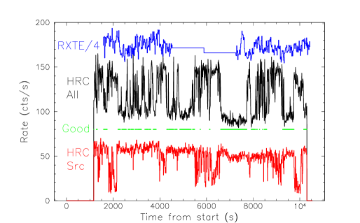
Figure 1.— GX13+1 lightcurve from HRC-I (red) and RXTE (in blue; divided by 4 for clarity). The full HRC-I field is shown in black, and the selected “good time intervals” are shown in green. When the full HRC-I spikes much above 100 cts/s, the telemetry limit affects the source count rate.

The extremely high flux from the source combined with the desire to get the highest possible spatial resolution required an unusual instrument configuration. In collaboration with the CXC Operations team, the HRC-I detector was positioned so that the source would appear in one corner of the HRC-I, while still being on-axis to the HRMA. This offset retained Chandra’s spatial resolution but ensured the source was far away from the normal aimpoint. Figure 2[Left] shows the full field of the HRC-I, with GX13+1 at one corner.

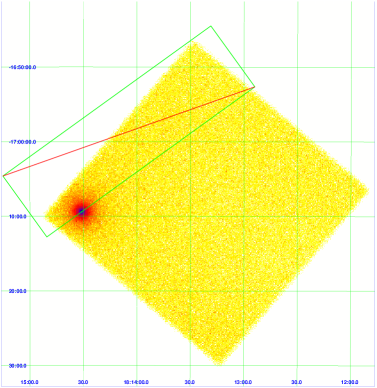
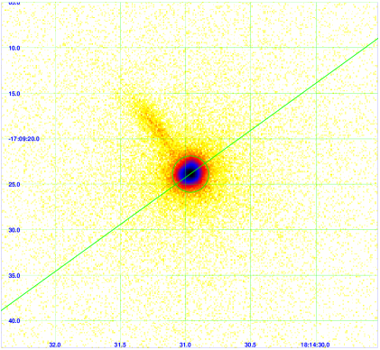
Figure 2.— [Left] The full HRC-I observation of GX13+1, with the excluded rectangular region marked. [Right] Expanded image of GX13+1 on the HRC-I, showing detector “jet” and excluded region. The 2” radius circle shows the near-source region excluded due to likely detector non-linearity.

In Figure 2[Right], a “jet”extending to the NE and containing $\sim 1000$ counts can be seen. This jet is a well-known detector artifact (Murray et al., 2000) which is normally removed by the standard processing to a level of $<0.1\%$ of the total source flux (Murray, 2000). In the case of GX13+1, this jet is $\sim 0.5\%$ of the apparent source count rate. The most likely cause is the high source count rate interfering with the the on-board electronic event processing (Dr. Michael Juda, private communication). Although the jet could be eliminated with aggressive filtering, this would also invalidate the standard calibration. It was therefore decided to simply ignore all events from the “jet”-side of the source, as shown by the box region in Figure 2[Left].

2.2. Extracting the Spectrum and Flux

The surface brightness of the X-ray halo must be normalized by the source flux to make absolute measurements of the dust column density. GX13+1 is observed almost constantly since it is a RXTE All-Sky Monitor (ASM) source with a average rate of 20-30 cts/s. However, as the RXTE ASM has little spectral sensitivity and the HRC-I has no effective energy resolution, simultaneous RXTE PCA observations of GX13+1 were taken to obtain a useful spectrum of the source. Although the RXTE PCA itself has only moderate resolution and little sensitivity below 2 keV, GX13+1’s spectrum is dominated by 2-4 keV photons (SES02). The PCA spectrum is shown in Figure 3[Left] as fit with a simple model consisting of an absorbed multi-color disk model plus a blackbody, following Ueda et al. (2004). The column density was fixed at the value found by Ueda et al. (2004) from the Chandra HETG, ${}_{\rm H}=3.2\times 10^{22}$ cm^-2, since this result is far more accurate than one obtained from the PCA. The best-fit inner temperature of the multicolor disk and the blackbody were 1.73 keV and 3.52 keV, with absorbed 1-10 keV fluxes of $7.43\times 10^{-9}$ erg cm^-2s^-1 and $2.30\times 10^{-10}$ erg cm^-2s^-1, respectively. Despite the large reduced $\chi^{2}_{\nu}$ ($>50$, driven by systematic errors), this model is an adequate fit for this work since only the total flux and the approximate spectral shape are needed to calculate the predicted response of the Chandra HRC-I. Nonetheless, it is important to note that fluxes measured with the RXTE PCA are systematically high by 10-15% in the 2-10 keV range, compared to other X-ray observatories (Jahoda, 2005).

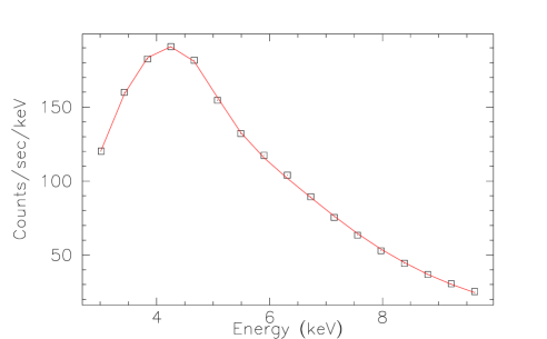
Figure 3.— [Left] The RXTE PCA spectrum of GX13+1, fit with an absorbed multicolor disk plus blackbody model. [Right] The best-fit model folded through the HRC-I response. The integrated count rate predicted is 64.6 cts/s.

To check the expected count rate, we folded this spectrum through the HRC effective area file for on-axis Cycle 7 data (hrciD2005-11-30pimmsN0008.fits), as shown in Figure 3[Right]. The total predicted source count rate in the HRC-I is 64.6 cts s^-1, $\sim 18$% larger than the observed HRC-I count rate of 54.8 cts s^-1 within 2’ of GX13+1. The discrepancy is primarily due to the overestimation from the RXTE PCA calibration, with an additional complication due to spatial variation in the response of the HRC-I that reduces the effective area of the detector corners relative to the center (Donnelly, Brown & Hole, 2003)

The Chandra PSF, measured as a ratio of the surface brightness to the source flux, is the background for this observation. The RXTE PCA, a non-imaging detector, includes both the direct source flux and the scattered halo photons, which must be removed to avoid double-counting. However, as the goal is to measure the scattered halo fraction itself, this problem is recursive. I addressed this by assuming a column density of $3.2\times 10^{22}$ cm^-2 and calculating the total scattered fraction for the MRN77, WD01, and ZDA04 BARE-GR-B models, weighted by the HRC-I response. The resulting halo fraction ranged from 13-26%. This predicted halo strength is consistent with the result that 22% of the total source counts are between $2^{\prime\prime}-120^{\prime\prime}$. Therefore, for purposes of calculating the background PSF, the RXTE PCA flux was reduced by 20% to exclude the halo contribution, with a 7% systematic error. This reduction is in addition to the 15% reduction described above. The 7% error is likely not the dominant term in the systematic error, however. The observation of a very bright source in one corner of the HRC-I detector is at the extreme edge of the available calibration, and so careful consideration of all uncertainties will be required.

Another concern regarding this observation was that a significant short-term change in the source flux, on the order of 12-24 hours, would also affect the halo in a time-delayed manner (e.g. Vaughan et al., 2004). At smaller angles the delay could be even longer. The RXTE ASM data was checked for a 10 day period before the observation, but no strong or significant variation was seen. Although Type I X-ray bursts have been seen from GX13+1 which show $3-4\times$ the normal flux, they only last $\sim 15$ seconds (Matsuba et al., 1995). In this case, no bursts were seen in either the HRC-I or PCA lightcurves, and indeed the halo observation would not be sensitive to such a small variation.

2.3. Point-spread function

An accurate measurement of the Chandra HRC-I point-spread-function (PSF) between 2-100” from the source is crucial to this observation. An accurate raytrace model (ChaRT ), of the Chandra HRMA has been calibrated for near-source ($<2^{\prime\prime}$) photons , SES02 showed that at large scattering angles this model significantly underestimates the PSF, leading to substantial problems in the analysis. Therefore, SES02 relied upon an ACIS-I observation of Her X-1 as a PSF calibrator, but this source is affected by pileup within $\sim 10$” and therefore cannot be used in the 2-10” range.

As shown in Figure 3[Right], the spectrum of GX13+1 peaks at $\sim 2$ keV. The HRC-I’s lack of spectral response means that spectral differences between any calibration source and GX13+1 will lead to additional complications. The best possible calibration source would be a bright, hard, and lightly-absorbed X-ray source observed on-axis with the HRC-I. The X-ray binary LMC X-1 matches these requirements reasonably well, and two Chandra observations (ObsID 1200, 1201) of the source have been done. However, they were both done early in the mission (August 1999) before the HRMA final focus was set and are thus unsuitable. Since then, the brightest hard X-ray source with little absorption and a known (albeit variable) flux to be observed with the HRC-I is 3C273 (ObsID 461 on Jan 22, 2000). Figure 4 shows 3C273’s surface brightness, divided by its source flux, as observed with the Chandra HRC-I (excluding the well-known jet region). The spectrum was taken from a Chandra HETG observation done twelve days earlier (ObsID 459) which is well-fit by an absorbed power-law with $\Gamma=1.67\pm 0.01$ and $F_{X}(2-10{\rm keV})=(1.08\pm 0.03)\times 10^{-10}$ ergs cm^-2s^-1. The absorption column was fixed at the Galactic value, N${}_{\rm H}=1.8\times 10^{20}$ cm^-2. The predicted HRC-I count rate (based on the CXC PIMMS tool) for this spectrum is 8.7 cts/s, while the actual source count rate was 26% higher at 11 cts/s. As the source is variable, this was taken as showing little change and the flux was simply assumed to have increased by 26% during the HRC-I observation. A significant but undetected change in the spectral shape could also cause this change in observed flux and might affect our results. However, BeppoSAX observations of 3C273 over a period of 10 days showed only small changes in the 2-10 keV spectral shape, with $\Gamma$ values ranging from $1.56\pm 0.02$ to $1.64\pm 0.02$ while the flux varied by 15% Haardt et al. (1998). The potential systematic error caused by uncertainty in the true spectrum of 3C273 during its observation with the HRC-I is thus smaller than the error due to unavoidable differences between the spectra of 3C273 and GX13+1.

The core of the PSF of 3C273 was fit with a Gaussian term centered at 0 with FWHM of $1.007_{-0.005}^{+0.004}$” and amplitude $1676\pm 42$ arcmin^-2. In addition, the best-fit model included two power-law terms with $\Gamma_{1}=4.06\pm 0.05,\Gamma_{2}=2.40_{-0.02}^{+0.01}$ and amplitudes $A_{1}=(3.4_{-0.9}^{+1.3})\times 10^{-7},A_{2}=(2.12_{-0.09}^{+0.13})\times 10^{-4}$ arcmin^-2 at 100”. The particle and sky background was fit with a constant, $(2.60\pm 0.02)\times 10^{-3}$ arcmin^-2. As Figure 4 shows the fit is quite good over a large range of surface brightnesses, with the somewhat large reduced $\chi^{2}_{\nu}=2.6$ likely due to the extreme precision of the measurement compared to the relatively simple model.

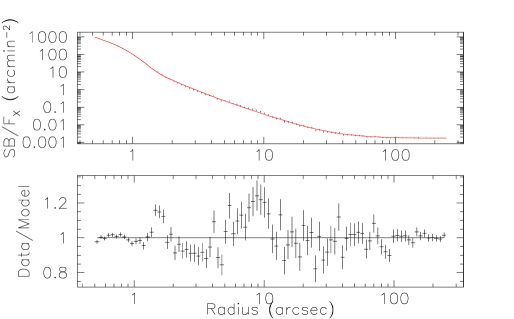
Figure 4.— [Top] The radial profile of 3C273’s surface brightness, divided by the source flux, fit with the sum of a Gaussian plus two power laws and a constant. [Bottom] The ratio of the data and model, showing small excursions at $1.5^{\prime\prime}$ and $10^{\prime\prime}$, but generally good agreement.

3. Results

The HRC-I observations are most useful between 2-100”, since beyond that radius the ACIS-I data can measure the energy-resolved X-ray halo. Therefore, the ACIS-I data were reprocessed (with CIAO 3.3) and reanalyzed following the approach described in SES02 except as noted below. Both the HRC-I and ACIS-I results were used in the final analysis. We note that in reprocessing the ACIS data, the source flux measurement, done via the CCD transfer “streak”, was redone with a better calibration and improved handling of the background subtraction which resulted in an overall $\sim 15$% decrease in the measured source flux. The calibration changes include a spatially-varying modification of order $\pm 5\%$ in the quantum efficiency uniformity in CALDB 2.28, and an energy-dependent increase of up to 16% in the overall effective area which was added in CALDB v3.2.1.

The data were fit using the CIAO fitting engine Sherpa using scattering models based on the exact Rayleigh-Gans (RG) approximation (Smith & Dwek, 1998). This model assumes the grains are spherical but uses the energy-dependent optical constants rather than the Drude approximation when calculating the scattering efficiency. Smith & Dwek (1998) noted that the full Mie treatment is necessary for X-rays $<2$ keV, since the RG overestimates the total scattering at low energies. The HRC-I is sensitive to X-rays between 0.08-10 keV, with peak efficiency between 0.7-2.0 keV. In all cases the halo model for the HRC-I was calculated using an average value weighted by the spectrum of GX13+1 and efficiency of the HRC-I. However, since GX13+1’s spectrum as observed by the HRC-I (see Figure 3[Right]) is dominated by photons with $E>2$ keV, the use of the simpler RG treatment is justified.

The initial analysis assumed the dust was smoothly distributed along the line of sight. Unlike SES02, where the predicted PSF was subtracted from the data, here the PSF was incorporated into the fitting directly to allow for an explicit inclusion of uncertainty in the PSF. Fits to the ACIS-I and HRC-I data included a constant factor that allowed for calibration uncertainty in the overall PSF, caused primarily by systematic errors in the source flux. For both the ACIS-I and HRC-I data this multiplier was allowed to vary by up to 10%. In many cases the fit pushed the multiplier to an extremum of the range, showing that systematic uncertainties remain in the data, although it is not clear what component dominates them. In SES02, systematic errors in the PSF manifested as energy-dependent column density fits, since to first order an error in the PSF could be adjusted by changing the overall halo scattering. As the total halo intensity is inversely proportional to energy, this effect is often a linear dependence of the best-fit N_H on energy. To check for this, I allowed the value of N_H to vary independently in the HRC-I and each energy band of the ACIS-I data. I used the F-test to determine that in only one case (ZDA04 BARE-GR-B) were the best-fit ACIS-I N_H values better described by a linear energy-dependent model than by a constant value. Even in this case, the F-test significance was only 3.5%, a negligible value given the number of different models tried. It seems unlikely, therefore, that there is a significant error in the relative power in the dust-scattered (halo) and mirror-scattered (PSF) photons.

Table 1 shows the best-fit N_H results for the HRC-I and the “average” ACIS-I value fit and the total $\chi^{2}_{\nu}$ assuming smoothly-distributed dust along the line of sight for the MRN77, WD01, and the 15 ZDA04 models. These can be compared to the value of $3.2\times 10^{22}$ cm^-2 found by Ueda et al. (2004). The ACIS-I column densities are $\sim 20\%$ larger than the HRC-I values, although the models with the lowest $\chi^{2}_{\nu}$ values tend to have the best agreement. The most likely cause of this discrepancy is cumulative errors in the source flux measurements combined with calibration differences between the ACIS-I and HRC-I detectors.

Table 1Smooth Dust Model Parameters

Model	NH(HRC)	NH(ACIS)	$\chi^{2}_{\nu}$
	$10^{22}$ cm-2	$10^{22}$ cm-2
MRN77	$2.4\pm 0.2$	$2.85\pm 0.05$	2.0
WD01	$1.51\pm 0.02$	$2.0\pm 0.2$	3.6
BARE-GR-S	$2.7\pm 0.2$	$2.9\pm 0.1$	1.9
BARE-GR-FG	$2.6\pm 0.2$	$3.00\pm 0.04$	1.9
BARE-GR-B	$3.6\pm 0.3$	$3.4\pm 0.4$	2.8
BARE-AC-S	$2.5\pm 0.2$	$3.0\pm 0.1$	2.1
BARE-AC-FG	$2.5\pm 0.1$	$3.0\pm 0.2$	2.2
BARE-AC-B	$3.3\pm 0.3$	$3.60\pm 0.05$	2.2
COMP-GR-S	$2.02\pm 0.02$	$2.9\pm 0.4$	4.9
COMP-GR-FG	$2.23\pm 0.04$	$3.0\pm 0.3$	3.5
COMP-GR-B	$3.0\pm 0.2$	$3.71\pm 0.09$	1.9
COMP-AC-S	$2.41\pm 0.02$	$3.7\pm 0.6$	7.0
COMP-AC-FG	$2.67\pm 0.02$	$3.8\pm 0.5$	5.0
COMP-AC-B	$4.24\pm 0.04$	$6.7\pm 0.9$	5.7
COMP-NC-S	$11.1\pm 0.6$	$13.5\pm 0.9$	2.4
COMP-NC-FG	$2.81\pm 0.02$	$4.6\pm 0.8$	8.6
COMP-NC-B	$3.39\pm 0.03$	$5.9\pm 1.1$	11.7

Figure 5 shows the profile of the HRC-I data along with the ACIS-I data at $2.5\pm 0.1$ keV, near the median energy of the spectrum as observed by the HRC-I. This figure shows the level of agreement between the HRC-I and ACIS-I data agree with each other in the overlap region ($50-100^{\prime\prime}$), as well as the large ($>20\times$) difference in the HRC-I and ACIS-I backgrounds in the $500-1000^{\prime\prime}$ region. The radial profile shown in Figure 5 is fit assuming the line of sight (LOS) dust is “smoothly-distributed” and has a composition and size distribution described by WD01 [Left], and the ZDA04 BARE-GR-S [Right] models. Although both models agree with the overall shape of the radial profile, the ratio plots show that the WD01 model underestimates the ACIS-I data in the $300-500^{\prime\prime}$ range, while the BARE-GR-S model underestimates the HRC-I data in the $10-50^{\prime\prime}$ range.

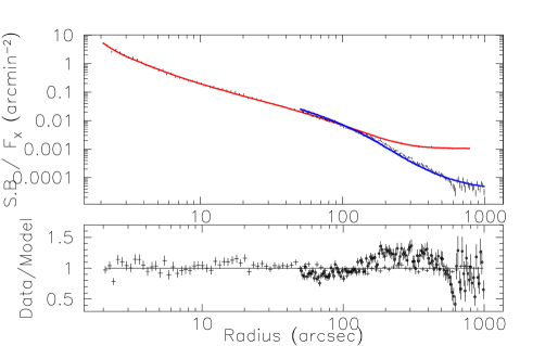
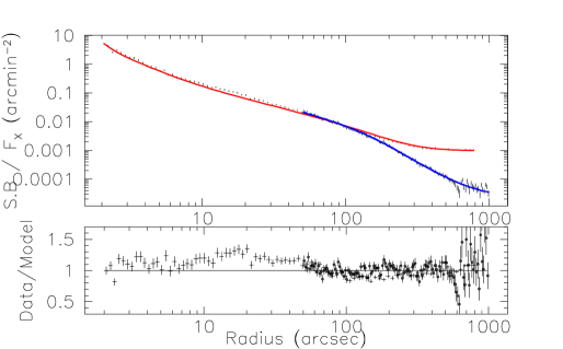
Figure 5.— [Left] The X-ray halo from smoothly-distributed WD01-type grains fit to the radial profile of GX13+1’s surface brightness divided by the source flux. The HRC-I observations are fit with a red line; the ACIS-I data (at 2.5 keV) with a blue line. The ratio of the HRC-I data to the model is shown below with crosses and the ACIS-I data with circles. [Right] Same, for the ZDA04 BARE-GR-S model.

The smoothly distributed dust fits show small discrepancies that might be indications of dusty molecular clouds along the line of sight. These would appear as “bumps” in the profile whose position and strength depends upon the relative distance to the cloud and its column density. I therefore refit the HRC-I and ACIS-I data using a two-component model that included a smoothly-distributed component plus a thin cloud with variable position and column density; the cloud is treated as a sheet with negligible thickness. Models using only a single thin cloud with no smooth component were also considered; these gave generally poor fits independent of the dust model used, and so were abandoned. This is not unexpected since (a) SES02 was unable to fit a single cloud using only the ACIS-I data and (b) GX13+1 is reasonably near the Galactic center ($(l,b)=(13.5^{\circ},0.1^{\circ})$, $D=7\pm 1$ kpc; Bandyopadhyay et al. (1999)) where a sightline dominated by a single cloud would be unusual.

To reduce fit time, the column density of both the smooth component and a cloud was fixed to be the same for all datasets, as was the position of the cloud along the line of sight. While more realistic than allowing the cloud column density to vary as a function of X-ray energy, this has the effect of magnifying residual systematic errors. As noted previously, the halo strength diminishes with energy while the relative PSF strength increases which can create a trend in the best-fit column density as a function of energy. However, since in only one case out of fourteen was such a trend seen previously, it seems unlikely that the systematic errors are driving the resulting best-fit parameters in the smooth plus cloud model.

The best-fit parameters for each model are shown in Table 2. None of the fits are formally acceptable ($\chi^{2}_{\nu}$ ranges from 2.1 to 9.9), although some are clearly better than others. In cases where the best-fit position is 0, the 1$\sigma$ upper limit is shown.

Table 2Smooth Plus Cloud Model Parameters

Model	NH(smooth)	NH(cloud)	Relative	$\chi^{2}_{\nu}$
	$10^{22}$ cm-2	$10^{22}$ cm-2	Position
MRN77	$2.60_{-0.05}^{+0.08}$	$0.69_{-0.03}^{+0.06}$	$<0.003$	2.4
WD01	$1.38\pm 0.02$	$0.46\pm 0.01$	$<0.001$	3.5
BARE-GR-S	$3.02\pm 0.01$	$0.15\pm 0.01$	$0.89\pm 0.01$	2.1
BARE-GR-FG	$2.95\pm 0.01$	$0.11\pm 0.01$	$0.91\pm 0.01$	2.2
BARE-GR-B	$3.51\pm 0.01$	$0.57\pm 0.01$	$0.82\pm 0.01$	2.4
BARE-AC-S	$2.6\pm 0.1$	$0.21\pm 0.06$	$<0.001$	2.4
BARE-AC-FG	$2.6\pm 0.1$	$0.23\pm 0.06$	$<0.001$	2.4
BARE-AC-B	$3.4\pm 0.1$	$0.35\pm 0.14$	$0.85\pm 0.01$	2.1
COMP-GR-S	$1.6\pm 0.1$	$0.82_{-0.09}^{+0.07}$	$<0.0003$	2.9
COMP-GR-FG	$2.0\pm 0.1$	$0.62_{-0.08}^{+0.06}$	$<0.004$	2.6
COMP-GR-B	$3.2\pm 0.1$	$0.23\pm 0.05$	$<0.01$	2.2
COMP-AC-S	$1.6_{-0.1}^{+0.2}$	$1.3\pm 0.1$	$<0.0002$	3.7
COMP-AC-FG	$2.2_{-0.1}^{+0.2}$	$1.0\pm 0.1$	$<0.0003$	3.3
COMP-AC-B	$2.9\pm 0.2$	$2.3\pm 0.1$	$<0.0004$	3.6
COMP-NC-S	$11.4_{-0.3}^{+0.6}$	$1.3\pm 0.3$	$<0.0008$	2.5
COMP-NC-FG	$1.6_{-0.2}^{+0.3}$	$1.9\pm 0.2$	$<0.0001$	4.3
COMP-NC-B	$1.6_{-0.5}^{+0.9}$	$2.5_{-0.5}^{+0.4}$	$<0.00001$	6.5

4. Discussion

Smith, Edgar & Shafer (2002) analyzed the ACIS-I observations of GX13+1’s dust scattered halo and found that the dust size distribution does not extend to very large ($>1\mu$m) grains and that grains do not have a large vacuum fraction. However, the ACIS-I data could not distinguish between the MRN77 and WD01 models, as the two distributions lead to similar scattering profiles at large angles. Similarly, the data left open the possibility that there might be a substantial population of grains near the source (Draine, 2003; Xiang et al., 2005). These would create a near-source scattered halo that was obscured by pileup in the ACIS-I detector. The primary goal of the HRC-I observation was to remove these uncertainties by measuring the halo near the source. This would determine which dust model best fit the data, as well as detecting (or put limits upon) variation in the dust distribution along the line of sight.

The fit results shown in Tables 1 and 2 contain a few surprises. Just as in Smith, Edgar & Shafer (2002), the WD01 model had the smallest column density of any of the models when fit with either smoothly distributed dust or after adding a cloud. However, the overall result was a significantly worse fit than found with either the MRN77 or many of the ZDA04 models. As Figure 5 shows, the smooth WD01 model fits the HRC data well, but underestimates the halo measured by ACIS between $150^{\prime\prime}-400^{\prime\prime}$, while the ZDA04 BARE-GR-S model underestimates the halo measured by the HRC between $10-50^{\prime\prime}$. Examining the other models show that these two cases are representative. Adding a single dust cloud to the model results in a solution with a cloud 70-90% of the distance to the source if the pure smooth model underestimates the halo around $30^{\prime\prime}$. Conversely, adding a cloud component to smooth dust models that underestimate the halo around $300^{\prime\prime}$ tend to put the cloud near the Sun.

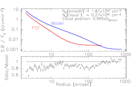
Figure 6.— [Top] Radial profile of GX13+1 from the HRC-I (upper points) with PSF calibration data from 3C273 (lower points). A close approximation to the Xiang et al. (2005) model for GX13+1 using the WD01 model is shown in blue, with the PSF fit to the 3C273 data is shown in red. [Bottom] Ratio of GX13+1 data to Xiang et al. (2005) model.

Although uncertainties remain due to calibration issues, the overall quality of the fits shown in Table 1 and Figure 5 do not support the proposition that a significant cloud of dust is present near GX13+1. In particular, although it is not identical to the Xiang et al. (2005) model, Figure 6 shows the result from a model similar to their fit to the zero-order HETG for GX13+1 using WD01-type dust. This approximation to their model puts a cloud with N${}_{\rm H}=2.7\times 10^{21}$ cm^-2 at a position 99.5% of the distance to GX13+1, along with a smooth distribution with N${}_{\rm H}=1.81\times 10^{22}$ cm^-2. In either their model or my approximation, the cloud near the source dominates the variation in the dust distribution. Figure 6 shows that although the HRC-I data contain an obvious halo, this model is not a good fit and, in fact, removing the cloud improves the fit. Although their model fit can be improved somewhat with a small vertical offset (corresponding to different relative flux calibrations of $\sim 12\%$), the model still predicts 10-20% more halo for $\theta<10^{\prime\prime}$ than is observed. Table 2 confirms this conclusion, finding (in the case of WD01-type dust) a cloud near the Sun, not the source, with N${}_{\rm H}\sim 5\times 10^{21}$ cm^-2.

ZDA04 described in detail how constraining dust models requires combining multiwavelength data from the IR to X-rays while simultaneously considering the metal abundances in the grains. Due to the nature of optical/UV extinction and X-ray scattering, few sources show strong signatures of dust in all of these wavebands (Valencic & Smith, 2007). Nonetheless, it is possible to constrain the allowed dust models by comparing the column density predicted by the models to that measured using other techniques. In the case of GX13+1, measurements of the column density range from $2.5-4.0\times 10^{22}$ cm^-2 (Charles & Naylor, 1992). Optical measurements provide only an upper limit of $2.9\times 10^{22}$ cm^-2 based on plausible but unconfirmed assumptions about the source spectrum(Garcia et al., 1992). The total H I column density through the Galaxy at the position of GX13+1 is $1.8\times 10^{22}$ cm^-2 (Dickey & Lockman, 1990), but this is misses the contribution from molecular H₂ that is likely to be substantial in the Galactic plane. The HETG observation of GX13+1 agrees (weakly) with these results (Ueda et al., 2004), although it does not strongly limit it. Only Mg can be directly measured ($N_{Mg}=1.84^{+0.91}_{-0.49}\times 10^{18}$ cm^-2), equivalent to ${\rm N}_{\rm H}$$=4.8^{+2.4}_{-1.3}\times 10^{22}$ cm^-2 assuming solar abundances. The $2\sigma$ upper limits for Si and S are equivalent to $\mbox{${\rm N}_{\rm H}$}<4\times 10^{22}$ cm^-2. Of course, LMXBs have shown significant variable internal absorption (Hertz & Grindlay, 1983) in X-rays, so this spectral measurement sets at best an upper limit to the actual interstellar component that is responsible for the halo.

Despite these difficulties in independently measuring the total LOS dust column density, we can reasonably justify excluding the value of N${}_{\rm H}=(1.11\pm 0.06)\times 10^{23}$ cm^-2 found in Table 1 for the ZDA04 COMP-NC-S model fit to the HRC-I data. However, this was only model from ZDA04 that used composite grains without bare carbon grains that had a plausible value of $\chi^{2}_{\nu}$. Although more data are needed, this class of models, along with the group of “composite grains with bare amorphous carbon” models are clearly suspect since they do not generate an X-ray halo similar to these observations. In fact, the only smoothly-distributed ZDA04 composite grains model that fit with $\chi^{2}_{\nu}<3$ had graphitic carbon and B star abundances (COMP-GR-B). After adding a dust cloud to the model, the COMP-GR-B model fit with $\chi^{2}_{\nu}=2.2$ while the next best fit (excluding the unrealistic COMP-NC-S model) was COMP-GR-FG with $\chi^{2}_{\nu}=2.6$, a significantly worse fit.

5. Conclusions

The principal results from this analysis are:

1. Although challenging, HRC-I observations can be used to recover the near-source region excluded by pileup in the ACIS-I detector. The lack of energy resolution can be finessed if another measurement of the source spectrum is available.

2. Fitting the source profile and background PSF independently improves overall results, since calibration uncertainties in the flux from the source and background objects can then be included explicitly.

3. There is no strong signature of a dust cloud at the source in the radial profile, as suggested by Xiang et al. (2005), although some models include a cloud $\sim 90$% of the distance to the source.

4. In agreement with SES02, the WD01 model underestimates the total column density to the source, and again leads to poor fits, although not so bad as to be excluded given the calibration uncertainties.

5. Some models from the ZDA04 paper, if not conclusively excluded, are at least implausible. In general, the ZDA04 models with composite grains (excepting the graphitic carbon model with B star abundances) gave poor fits, while the bare carbon and silicate grain models tended to fit well.

It should be noted that the relatively good fits found using the simple smoothly-distributed dust model are somewhat surprising, since X-ray halos probe both the largest grains whose size and composition are the least constrained from observations in other wavelengths. Additionally, X-ray halos are primarily observed through highly-absorbed lines of sight. These probe dust in dense molecular clouds that cannot be observed in the optical or UV due to the extremely large extinction. Finally, all of these models assume spherical grains, although recently some calculations have been done on aspherical grains (Draine & Allaf-Akbari, 2006) that show the effects are small ($<20\%$) for the WD01 model at $\sim 2$ keV. Despite these potential problems, a number of existing grain models agree quite well with the observations, suggesting grains in dense clouds (with the exception of the densest regions that take up very little volume and may be optically-thick to X-rays) are not too dissimilar from grains in less dense regions.

References

- Bandyopadhyay et al. (1999) Bandyopadhyay, R. M., Shahbaz, T., Charles, P. A. & Naylor, T. 1999, MNRAS, 306, 417
- Chandra X-ray Center (2006) Chandra X-ray Center Proposer’s Guide, v 9.0 2006, http://asc.harvard.edu/proposer/POG/html/HRC.html
- Charles & Naylor (1992) Charles, P. A. & Naylor, T. 1992, MNRAS 255, 6
- Dickey & Lockman (1990) Dickey, J. M. & Lockman, F. J. 1990, ARA&A, 28, 215
- Donnelly, Brown & Hole (2003) Donnelly, R. H., Brown, J. P. & Hole, K. T. 2003, http://asc.harvard.edu/cal/Hrc/Documents/hrci_qeu.ps
- Draine (2003) Draine, B. T. 2003, ApJ, 598, 1026
- Draine & Allaf-Akbari (2006) Draine, B. T., & Allaf-Akbari, K. 2006, ApJ, 652, 1318
- Garcia et al. (1992) Garcia, M. R. et al. 1992, AJ, 103, 1325
- Haardt et al. (1998) Haardt, F. et al. 1998, A&A, 340, 35
- Henke, Gullikson & Davis (1993) Henke, B. L., Gullikson, E. M. & Davis, J. C. 1993, ADNDT, 54, 2
- Hertz & Grindlay (1983) Hertz, P. & Grindlay, J. 1983, ApJ, 275, 105
- Jahoda (2005) Jahoda, K. 2005, http://astrophysics.gsfc.nasa.gov/xrays/programs/ rxte/pca/flux_scale.pdf
- Landgraf et al. (2000) Landgraf, M., Baggaley, W. J., Grün, E., Krg̈er, H., & Linkert, G. 2000 J. Geophys. Res., 105, 10343
- Mathis & Whiffen (1989) Mathis, J. S. & Whiffen, G. 1989, ApJ, 341, 808
- Mathis & Lee (1991) Mathis, J. S. & Lee, C. W. 1991, ApJ, 376, 490
- Mathis, Rumpl & Nordsieck (1977) Mathis, J. S., Rumpl, W. & Nordsieck, K. H. 1977, ApJ, 280, 425
- Murray et al. (2000) Murray, S. S., et al. 2000, Proc. SPIE, 4140, 144
- Murray (2000) Murray, S. S. 2000, http://cxc.harvard.edu/cal/Hrc/Documents/ghosts.ps
- Matsuba et al. (1995) Matsuba, E. et al. 1995, PASJ, 47, 575
- Smith & Dwek (1998) Smith, R. K. & Dwek, E. 1998, ApJ, 503, 831