Measuring the cosmological parameters with the – correlation of Gamma–Ray Bursts
Abstract
We have used the – correlation of GRBs to measure the cosmological parameter M. By adopting a maximum likelihood approach which allows us to correctly quantify the extrinsic (i.e. non–Poissonian) scatter of the correlation, we constrain (for a flat universe) M to 0.04–0.40 (68% confidence level), with a best fit value of M , and exclude M = 1 at 99.9% confidence level. If we release the assumption of a flat universe, we still find evidence for a low value of M (0.04–0.50 at 68% confidence level) and a weak dependence of the dispersion of the – correlation on Λ (with an upper limit of Λ at 90% confidence level). Our approach makes no assumptions on the – correlation and it does not use other calibrators to set the “zero’ point of the relation, therefore our treatment of the data is not affected by circularity and the results are independent of those derived via type Ia SNe (or other cosmological probes). Unlike other multi-parameters correlations, our analysis grounds on only two parameters, then including a larger number (a factor ) of GRBs and being less affected by systematics. Simulations based on realistic extrapolations of ongoing (and future) GRB experiments (e.g., Swift, Konus–Wind, GLAST) show that: i) the uncertainties on cosmological parameters can be significantly decreased; ii) future data will allow us to get clues on the “dark energy” evolution.
keywords:
gamma–rays: observations – gamma–rays: bursts – cosmology: cosmological parameters.1 Introduction
Gamma–ray Bursts (GRBs) are the brightest cosmological sources in the universe, with isotropic luminosities up to 1054 erg cm-2 s-1and a redshift distribution extending at least up to 6.3 (e.g., Tagliaferri et al. 2005). Thus, these sources may be interesting for cosmological studies, if one can use them to provide measurements of the cosmological parameters independently of other methods, like the CMB (e.g., De Bernardis et al. 2000; Spergel et al. 2003; Dunkley et al. 2008 ; Komatsu et al. 2008), type Ia SN (e.g., Perlmutter et al. 1998; Perlmutter et al. 1999; Riess et al. 1998; Riess et al. 2004; Astier et al. 2006), Baryon Acoustic Oscillations (BAO) (e.g., Eisenstein et al. 2005; Tegmark et al. 2006; Percival et al. 2007), galaxy clusters (e.g., Rosati, Borgani & Norman 2002; Voit 2005). However, GRBs are not standard candles, given that their luminosities span several orders of magnitude under the assumption of both isotropic and collimated emission ( e.g., Ghirlanda et al. 2006). In the recent years, several attempts to ”standardize” GRB have been made, mainly on the basis of correlations involving: a) a GRB intensity indicator, like the isotropic–equivalent radiated energy () or the isotropic–equivalent peak luminosity (); b) the photon energy at which the time averaged Fν spectrum peaks (”peak energy”, ); c) other observables, like the break time of the afterglow light curve, tb, or the ”high signal time scale” T0.45 (Ghirlanda, Ghisellini & Lazzati, 2004; Firmani et al., 2006). Finally, Schaefer (2007) used different correlations (spectrum–energy, time lag – luminosity, peak luminosity – variability) to construct a GRB Hubble diagram and constrain the cosmological parameters.
These analyses have provided useful constraints on M and Λ consistent with those derived from type Ia SNe, see, e.g., Ghirlanda et al. (2006) for a review. However, the use of these correlations for cosmology is controversial. For example, because of the lack of low redshift GRBs they cannot be directly calibrated. On the other hand the calibration of a spectrum–energy correlation using SNe-Ia as calibrators (Kodama et al., 2008; Liang et al., 2008) is an interesting attempt to use GRBs as cosmological probes, but it may look suspicious that this method gives very similar results to those obtained via SNe. Thus, particular care and sophisticated statistical methodologies have to be adopted in order to avoid circularity problems when constructing a GRB Hubble diagram. In addition, recent analyses based on updated samples of GRBs showed that the dispersion of three–parameter correlations could be significantly larger than thought before (Campana et al., 2007; Ghirlanda et al., 2007; Rossi et al., 2008).
In this article we investigate the possibility of constraining the cosmological parameters from the – correlation. This correlation was initially discovered on a small sample of BeppoSAX GRBs with known redshift (Amati et al., 2002) and confirmed afterwards by Swift observations (Amati, 2006). Although it was the first ”spectrum–energy” correlation discovered for GRBs (and the most firmly established one, to date) it was never used for cosmology purposes, because of its significant ”extrinsic” scatter (i.e., a scatter in excess to the ”intrinsic” Poissonian fluctuations of the data). However, the conspicuous increasing of GRB discoveries combined with the fact that – correlation needs only two parameters that are directly inferred from observations (this fact minimizes the effects of systematics and increases the number of GRBs that can be used, by a factor ) makes the use of this correlation an interesting tool for cosmology.
Our study was motivated by our finding that, in the assumption of a flat universe, the obtained by fitting the – correlation with a power-law varies with the value of M assumed to compute , has its minimum value for M0.25, very close the value obtained with SNe-Ia approach. In this paper we show indeed that a small fraction of the extrinsic scatter is due to to the choice of cosmological parameters, thus allowing us to constrain M and, to a smaller extent, Λ.
| GRB | Fluence(a) | (b) | Instruments | Refs. for (c) | ||
|---|---|---|---|---|---|---|
| (10-5 erg cm-2) | (keV) | (1052 erg) | spectrum | |||
| 970228 | 0.695 | 1.30.1 | 19564 | 1.600.12 | SAX | (1) |
| 970508 | 0.835 | 0.340.07 | 14543 | 0.610.13 | SAX | (1) |
| 970828 | 0.958 | 12.31.4 | 586117 | 293 | GRO | (1) |
| 971214 | 3.42 | 0.870.11 | 685133 | 213 | SAX | (1) |
| 980326 | 1.0 | 0.180.04 | 71 | 0.48 | SAX | (1) |
| 980613 | 1.096 | 0.190.03 | 19489 | 0.590.09 | SAX | (1) |
| 980703 | 0.966 | 2.90.3 | 50364 | 7.20.7 | GRO | (1) |
| 990123 | 1.60 | 35.85.8 | 1724466 | 22937 | SAX/GRO/KW | (1) |
| 990506 | 1.30 | 21.72.2 | 677156 | 949 | GRO/KW | (1) |
| 990510 | 1.619 | 2.60.4 | 42342 | 173 | SAX | (1) |
| 990705 | 0.842 | 9.81.4 | 459139 | 183 | SAX/KW | (1) |
| 990712 | 0.434 | 1.40.3 | 9315 | 0.670.13 | SAX | (1) |
| 991208 | 0.706 | 17.21.4 | 31331 | 22.31.8 | KW | (1) |
| 991216 | 1.02 | 24.82.5 | 648134 | 677 | GRO/KW | (1) |
| 000131 | 4.50 | 4.70.8 | 987 416 | 17230 | GRO/KW | (1) |
| 000210 | 0.846 | 8.00.9 | 75326 | 14.91.6 | KW | (1) |
| 000418 | 1.12 | 2.80.5 | 28421 | 9.11.7 | KW | (1) |
| 000911 | 1.06 | 23.04.7 | 1856371 | 6714 | KW | (1) |
| 000926 | 2.07 | 2.60.6 | 31020 | 27.15.9 | KW | (1) |
| 010222 | 1.48 | 14.61.5 | 76630 | 819 | KW | (1) |
| 010921 | 0.450 | 1.80.2 | 12926 | 0.950.10 | HET | (1) |
| 011121 | 0.36 | 24.36.7 | 1060265 | 7.82.1 | SAX/KW | (2) |
| 011211 | 2.14 | 0.500.06 | 18624 | 5.40.6 | SAX | (1) |
| 020124 | 3.20 | 1.20.1 | 448148 | 273 | HET/KW | (1) |
| 020405 | 0.69 | 8.40.7 | 35410 | 100.9 | SAX/KW | (2) |
| 020813 | 1.25 | 16.34.1 | 590151 | 6616 | HET/KW | (1) |
| 020819B | 0.410 | 1.60.4 | 7021 | 0.680.17 | HET | (1) |
| 020903 | 0.250 | 0.0160.004 | 3.371.79 | 0.00240.0006 | HET | (1) |
| 021004 | 2.30 | 0.270.04 | 266117 | 3.30.4 | HET | (1) |
| 021211 | 1.01 | 0.420.05 | 12752 | 1.120.13 | HET/KW | (1) |
| 030226 | 1.98 | 1.30.1 | 28966 | 12.11.3 | HET | (1) |
| 030323 | 3.37 | 0.120.04 | 270113 | 2.80.9 | HET | (3) |
| 030328 | 1.52 | 6.40.6 | 32855 | 473 | HET/KW | (1) |
| 030329 | 0.17 | 21.53.8 | 10023 | 1.50.3 | HET/KW | (1) |
| 030429 | 2.65 | 0.140.02 | 12826 | 2.160.26 | HET | (1) |
| 030528 | 0.78 | 1.40.2 | 579.0 | 2.50.3 | HET | (3) |
| 040912 | 1.563 | 0.210.06 | 4433 | 1.30.3 | HET | (4) |
| 040924 | 0.859 | 0.490.04 | 10235 | 0.950.09 | HET/KW | (1) |
| 041006 | 0.716 | 2.30.6 | 9820 | 3.00.9 | HET | (1) |
| 050318 | 1.44 | 0.420.03 | 11525 | 2.200.16 | SWI | (1) |
| 050401 | 2.90 | 1.90.4 | 467110 | 357 | KW | (1) |
| 050416A | 0.650 | 0.0870.009 | 25.14.2 | 0.100.01 | SWI | (1) |
| 050525A | 0.606 | 2.60.5 | 12710 | 2.500.43 | SWI | (1) |
| 050603 | 2.821 | 3.50.2 | 1333107 | 604 | KW | (1) |
| 050820 | 2.612 | 6.40.5 | 1325 | 97.47.8 | KW | (5) |
| 050904 | 6.29 | 2.00.2 | 31781094 | 12413 | SWI/KW | (6) |
| 050922C | 2.198 | 0.470.16 | 415111 | 5.31.7 | HET | (1) |
| 051022 | 0.80 | 32.63.1 | 754258 | 545 | HET/KW | (1) |
| 051109A | 2.346 | 0.510.05 | 539200 | 6.50.7 | KW | (1) |
| 060115 | 3.53 | 0.250.04 | 28534 | 6.30.9 | SWI | (7) |
| 060124 | 2.296 | 3.40.5 | 784285 | 41 6 | KW | (8) |
| 060206 | 4.048 | 0.140.03 | 39446 | 4.30.9 | SWI | (7) |
| 060218 | 0.0331 | 2.20.1 | 4.90.3 | 0.00530.0003 | SWI | (9) |
| 060418 | 1.489 | 2.30.5 | 572143 | 133 | KW | (10) |
| GRB | Fluence(a) | (b) | Instruments | Refs. for (c) | ||
|---|---|---|---|---|---|---|
| (10-5 erg cm-2) | (keV) | (1052 erg) | spectrum | |||
| 060526 | 3.21 | 0.120.06 | 10521 | 2.60.3 | SWI | (11) |
| 060614 | 0.125 | 5.92.4 | 5545 | 0.210.09 | KW | (12) |
| 060707 | 3.425 | 0.230.04 | 27928 | 5.41.0 | SWI | (7) |
| 060814 | 0.84 | 3.80.4 | 473155 | 7.00.7 | KW | (13) |
| 060908 | 2.43 | 0.730.07 | 514102 | 9.80.9 | SWI | (7) |
| 060927 | 5.60 | 0.270.04 | 47547 | 13.82.0 | SWI | (7) |
| 061007 | 1.261 | 21.12.1 | 890124 | 869 | KW/SUZ | (14) |
| 061121 | 1.314 | 5.10.6 | 1289153 | 22.52.6 | KW/SUZ | (15) |
| 061126 | 1.1588 | 8.71.0 | 1337410 | 303 | SWI/RHE | (16) |
| 070125 | 1.547 | 13.31.3 | 934148 | 80.28.0 | KW | (17) |
| 071010B | 0.947 | 0.740.37 | 10120 | 1.70.9 | KW | (18) |
| 071020 | 2.145 | 0.870.40 | 1013160 | 9.54.3 | KW | (19) |
| 071117 | 1.331 | 0.890.21 | 647226 | 4.10.9 | KW | (20) |
| 080319B | 0.937 | 49.73.8 | 126165 | 1149 | KW | (21) |
| 080319C | 1.95 | 1.50.3 | 906272 | 14.12.8 | KW | (22) |
| 080411 | 1.03 | 5.70.3 | 52470 | 15.60.9 | KW | (23) |
-
Notes. (a) Bolometric fluence computed in the [ – ] keV energy range.
(b) Computed by assuming H0 =70 km s-1 Mpc-1, M = 0.3 and Λ = 0.7 .
(c)References for the spectral parameters and for the values and uncertainties of and : (1) Amati (2006) and references therein; (2) Ulanov et al. (2005) and refined analysis of BeppoSAXdata; (3) Sakamoto et al. (2005); (4) Stratta et al. (2006); (5) Cenko et al. (2006); (6) Krimm et al. (2006); (7) Sakamoto et al. (2008a); (8) Golenetskii et al. (2006a); (9) Campana et al. (2006); (10) Golenetskii et al. (2006b); (11) Schaefer (2007) and references therein; (12) Amati et al. (2007) and references therein; (13) Golenetskii et al. (2006c); (14) Mundell et al. (2007) and references therein; (15) Ghirlanda et al. (2007) and references therein; (16) Perley et al. (2008); (17) Golenetskii et al. (2007a); (18) Golenetskii et al. (2007b); (19) Golenetskii et al. (2007c); (20) Golenetskii et al. (2007d); (21) Golenetskii et al. (2008a); (22) Golenetskii et al. (2008b); (23) Golenetskii et al. (2008c).
 ,
,
2 The updated – sample
Previous analyses of the – plane of GRBs shows that different classes of GRBs exhibit different behaviours: while normal long GRBs and X–Ray Flashes (XRF, i.e. particularly soft bursts) follow the – correlation, short GRBs and the peculiar very close and sub–energetic GRB 980425 do not (Amati et al. 2007). Therefore, in our analysis we considered only long GRB/XRF. The sample of long GRB/XRF used in this paper (updated to April, 11 2008) is reported in Table 1 and includes 70 GRBs. We report, for each GRB, the redshift, the fluence and the cosmological rest–frame spectral peak energy, =(1+). The redshift distribution covers a broad range of , from 0.033 to 6.3, thus extending far beyond that of Type Ia SNe (z 1.7). For Swift GRBs, the value derived from BAT spectral analysis alone were conservatively taken from the results reported by the BAT team (Sakamoto et al., 2008a, b). Other BAT values reported in the literature were not considered, because either they were not confirmed by Sakamoto et al. (2008a, b) refined analysis (e.g., Cabrera et al. 2007) or they are based on speculative methods (Butler et al., 2007).
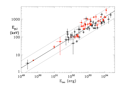
In Table 1 we also report the values of computed from published spectral parameters and fluences by following the standard method described, e.g., by Amati (2006) and assuming H km s-1 Mpc-1, and (references are reported in Table 1). An analysis of Figure 1 (left panel) shows that, for this ”standard” cosmology, all GRBs in our sample follow the – correlation; in particular, Swift GRBs are well consistent with the – correlation based on GRBs discovered by other instruments characterised by different trigger thresholds and sensitivities (as a function of energy). This fact points out that the – correlation is not affected by significant selection effects (see also Ghirlanda et al. 2008).
If we fit the data of Figure 1 with a simple power–law, we find an index and a normalization , consistent with results of previous analyses (e.g., Amati 2006). However, despite the very high significance of the correlation (Spearman’s for 70 events), the fit with a power–law provides an highly unacceptable value (408/68). This is clear evidence of the existence of a significant extrinsic scatter, which is superimposed to the Poissonian one and implies the existence of ”hidden” parameters, connected with GRB phenomenology, which contribute to define the location of a GRB in the – plane. It should be noted that systematics affecting both and may contribute to the extrinsic scatter, even if there is evidence that they are not a dominant component (Landi et al., 2006).



3 Cosmological parameters derived from the – correlation
The main goal of this paper is to investigate if the extrinsic dispersion of the – correlation is sensitive at varying the values of the cosmological parameters M and Λ. We emphasize that this method does not suffer from circularity, since we do not assume an – relation based on a particular choice of the cosmological parameters or calibrate it by using other cosmological probes.
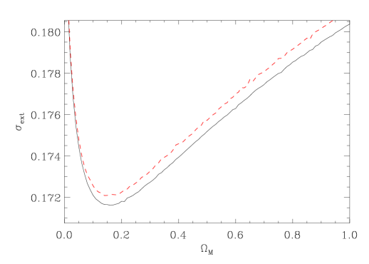
As a first step, under the assumption of a flat universe, we studied the trend of the values obtained by fitting the – correlation with a simple power–law, for different choices of M. Here and in the the following, we assumed H0 = 70 km s-1 Mpc-1. Figure 2 (left) shows that the extrinsic scatter of the correlation indeed decreases with cosmology, and minimizes for M 0.25. This result is in qualitative agreement with the one obtained, e.g., with SNe (Perlmutter et al., 1998, 1999; Riess et al., 1998, 2004; Astier et al., 2006).
In order to better characterize the dependence of the – extrinsic scatter on cosmology, we have used the maximum likelihood method (hereafter MLM) as discussed by D’Agostini (2005) (see also Guidorzi et al. 2006, Amati 2006 and Rossi et al. 2008 for other applications of this methodology). This method assumes that, if the correlated data (xi,yi) can be described by a linear function with the addition of an extrinsic scatter ext among the free parameters, the optimal values of the parameters (, , and ext) can be obtained by minimizing the –log(likelihood) function, in which the uncertainties on both (xi,yi) are taken into account. The general log(likelihood) function is given by:
| (1) |
where, in our case, log(), x = 0 and y = ext. We remark that setting x = 0 does not affect the general validity of this formula.
As an example, the fit of the correlation with this method by using the values reported in Table 1 provides the following parameters value: , and (68% c.l.; consistent with the results reported by Amati 2006 for a smaller sample of 41 GRBs). In Figure 1 (right) we show the distribution of the normalised scatter of the data (see, e.g., Rossi et al. 2008 for details on the computation of this quantity) with superimposed the normalised Gaussian. It is apparent that the scatter of the – correlation is indeed dominated by the extrinsic (i.e. non–Poissonian) variance.
For the goals of this paper, we repeated the above analysis by varying M, always under the assumption of a flat universe. Figure 2 (right) and Figure 3 (left) show that the values of the –log(likelihood) and of the extrinsic variance ext are indeed sensitive to M, both showing a clear minimum around M 0.15. Also the slope of the correlation is sensitive to the adopted cosmology, as shown in Figure 3 (right). By using the probability density function, the MLM also allows us to constrain M, that results to be in the range 0.04–0.40 at 68% and in the range 0.02–0.68 at 90% c.l (Table 2). An M value of 1 can be exluded at 99.9% c.l.
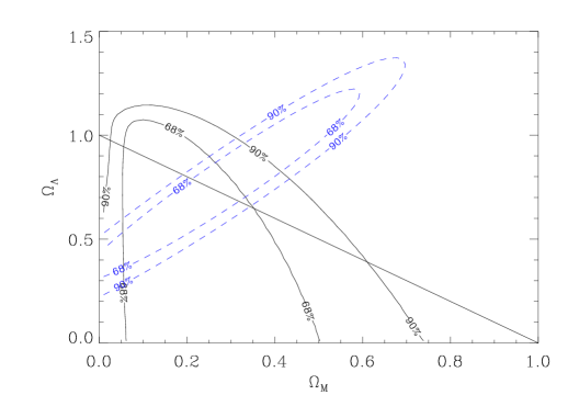
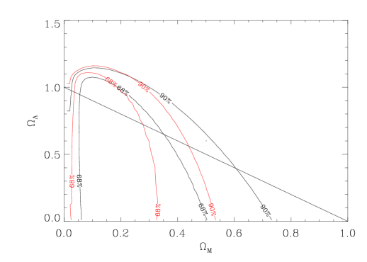
If we release the flat universe hypothesis and let M and Λ vary independently (Figure 4, left), we still find evidence for an universe with a low value of M (0.04–0.50 at 68% c.l.). Only an upper limit of 1.05 can be set to Λ (see Table 2). This fact is not surprising, given that the redshift distribution of GRBs is expected to produce very vertically elongated contours in the M – Λ plane (Ghirlanda et al., 2006; Kodama et al., 2008). The complementarity of GRB with other cosmological probes can be seen in Figure 4, where we plot, in addition to our results, the contours derived from SN Ia by Astier et al. (2006). As can be seen, already with the present sample of GRB, significantly improved constraints on M can be obtained by the combination of the two probes.
We have also investigated the estimate of the free paramaters of the the inverse relation plus the extrinsic scatter parameter . The results are fully consistent with previous ones and satisfy the expectation that , where is the Pearson’s weighted linear-correlation coefficient (e.g., Bevington 1969, Bendat & Piersol 2000). For a flat universe with M= 0.3, we find , , and .
Finally, we tested our results using the likelihood function suggested by Reichart (2001). The results obtained are fully consistent with the results above (Figure 2, left). This shows that the constraints that we have derived on the cosmological parameters do not depend significantly on the adopted statistical methodology and confirms the general soundness of our approach.
| Method | c.l. | M(flat) | M | Λ |
|---|---|---|---|---|
| scatter | 68% | 0.04 – 0.40 | 0.04 – 0.50 | 1.05 |
| 90% | 0.02 – 0.68 | 0.01 – 0.75 | 1.15 | |
| scatter | 68% | 0.04 – 0.40 | 0.05 – 0.41 | 1.05 |
| (self calib.) | 90% | 0.02 – 0.67 | 0.01 – 0.73 | 1.13 |
| scatter | 68% | 0.03 – 0.28 | 0.03 – 0.33 | 1.10 |
| () | 90% | 0.01 – 0.49 | 0.01 – 0.53 | 1.17 |

4 Future perspectives
4.1 Enrichment and redshift extension of the sample
In order to estimate the accuracy on cosmological parameters achievable by ongoing and future experiments, we have carried out a number of simulations based on an enriched sample of GRBs. By using the slope, normalization and extrinsic scatter of the – correlation obtained with the real sample of 70 GRBs and assuming, as an example, M=0.27, Λ=0.73, we generated 150 random GRBs with an accuracy on and of 20%. For 90% of the simulated GRBs, the redshift was randomly chosen from the GRB redshift distribution of our sample. For the remaining 10% of simulated GRBs we assumed a value of redshift larger than 6. The number of GRBs, and the accuracy on and , of the simulated sample are those that will realistically be provided in the next years by joint observations of Swift and GLAST/GBM (plus also Konus-Wind, Suzaku, RHESSI, AGILE, etc.). Also the extension of the redshift distribution up to at least is consistent both with theoretical predictions based on star formation rate evolution and the expected improvement in the sensitivity of hard X–ray and optical/near–infrared telescopes, that will be used to detect and follow–up GRBs and measure GRB redshift (e.g., Salvaterra et al. 2007 Salvaterra & Chincarini 2007).
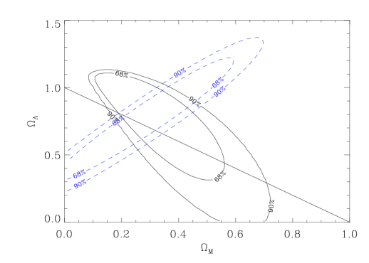
In Figure 4 (right) we show the confidence level contours for Mand Λ obtained by applying the method described in Section 3 to the sample made of the 70 “real” GRBs plus the 150 “simulated” ones. In Table 3, we report the constraints on cosmological parameters both in the assumption of a flat universe and by varying simultaneously M and Λ. A simple comparison with Table 2 shows that the simulated sample decreases the uncertainty range of M from 10 to only a factor 2. In addition, as can be seen in Figure 4 (right), significantly improved constraints on both M and Λ will be obtained by the combination of the contours obtained from GRBs with those from other probes, like, e.g., SN Ia.
Finally we note that the – correlation, because it needs the measure of a third observable (i.e. the break time in the optical afterglow light curve) requires the estimates of and for a number of GRBs larger by more than a factor of 3 than required by the – correlation. For instance, the simulations performed by Ghirlanda et al. (2006) with 150 GRBs correspond to a “real” sample of at least 500 GRBs having both and measured.
4.2 Calibrating the – correlation
One of the main problems with the use of GRB correlations for cosmology is the lack of low–redshift GRBs (i.e. lying at z 1) allowing for a cosmology–independent calibration similarly to type Ia SNe. This problem can be partly overcome by fitting the correlation in a sub–sample of GRBs lying at similar redshifts. This technique was proposed for future calibration of the slope of the – correlation (e.g., Ghirlanda et al. 2006), but can be effectively used for the – correlation, due to the much larger number of events that can be included in the – sample with respect to the – one. By studying the redshift distribution of the GRBs in our sample, we find that there are 18 events lying at redshift between 0.8 and 1.2. The analysis of this sub–sample with the MLM method provides, indeed, evidence of a very low variation of as a function of cosmological parameters. For instance, by assuming a flat universe, we find that the best–fit values are in the range =0.493–0.496, to be compared to =0.477–0.560 obtained on the whole sample of 70 GRB. The value of holds stable within this interval even by varying both M and Λ in the [0,1] range. The dependence of on the dark energy equation of state (parametrised as discussed in next section) is also within this interval. However, when taking into account the uncertainty resulting from the fits, the constraint on the calibrated slope of the – correlation becomes larger: = 0.44–0.55, for both a flat and general universe. Thus, the applicability of the method is currently hampered by the large uncertainty affecting , which results in a marginal improvements of the c.l. of cosmological parameters (Figure 5, left; Table 2). On the other hand, if we apply this calibration method to the simulated sample of 70 + 150 GRB, the improvement in the estimates of cosmological parameters is significant (see Table 3 and compare Figure 5, right, with Figure 4, right).
A second possibility to calibrate the slope of the correlation is to derive it on robust physical basis. Several analyses reported above or elsewhere (e.g., Ghirlanda et al. 2008) point out a slope of =0.5. This value is also predicted by several theoretical models, involving in various forms synchrotron, inverse Compton, thermal and Comptonised thermal emissions; see, e.g., Zhang & Mészáros (2002); Thompson et al. (2007). Figure 5 (red contours) and Table 3 illustrate quite clearly that the correlation fitted with the MLM method after assuming improves significantly the accuracy degree of the cosmological parameter measurements.
4.3 Investigating the evolution of the dark energy
The GRB redshift distribution extends up to , which is well above that of SNe-Ia (). Therefore, at least in principle, GRBs are powerful tools to study the evolution of dark energy with the redshift. In the following, we adopt the parametrization of the dark energy equation of state proposed by Chevallier & Polarski (2001); Linder & Utherer (2005), i.e. , where:
| (2) |
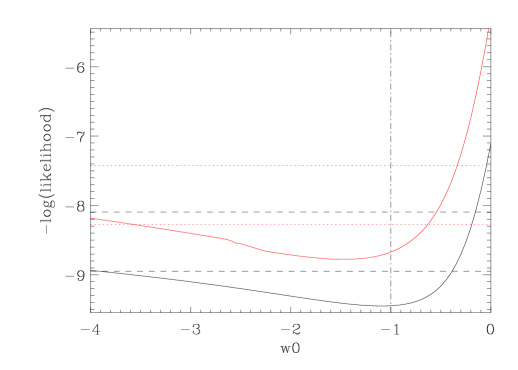
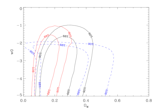
As shown in Figure 6 (left), with our sample of 70 GRBs we find that the –log(likelihood) computed with the MLM by assuming a flat universe with M = 0.27 and by setting = 0 is indeed sensitive to , with a minimum around (corresponding to a cosmological constant). Unfortunately, within the limits of present GRB sample no significant constraints on can be provided. Even after assuming , can be constrained only to be between 3.7 and 0.7 at 68% c.l. In Figure 6 (right) we show the M – confidence level contours obtained with the sample of 70 real + 150 simulated GRBs by assuming a flat universe with = 0 (continuous lines) and = 4 (dashed line). As can be seen, such a sample would provide clear evidence of 1 and some hints on .
| Method | c.l. | M(flat) | M | Λ |
|---|---|---|---|---|
| scatter | 68% | 0.21 – 0.50 | 0.11 – 0.57 | 0.35 – 1.12 |
| 90% | 0.16 – 0.66 | 0.08 – 0.73 | 1.15 | |
| scatter | 68% | 0.22 – 0.48 | 0.12 – 0.49 | 0.47 - 1.10 |
| (self calib.) | 90% | 0.17 – 0.59 | 0.10 – 0.69 | 0.10 - 1.11 |
| scatter | 68% | 0.13 – 0.27 | 0.18 – 0.28 | 0.62 – 1.10 |
| () | 90% | 0.11 – 0.35 | 0.06 – 0.35 | 0.50 – 1.12 |
5 Conclusions
We have used an updated sample of 70 GRBs aimed at deriving the cosmological parameters M and Λ from the – correlation of GRBs. With respect to previous attempts mainly based on the – and – –T0.45 correlations, the use of – correlation has the advantages of requiring only two parameters, both directly inferred from observations. This fact allows for the use of a richer sample of GRBs (e.g., a factor 3-4 larger than used in the – correlation), and a reduction of systematics, with respect to three–parameters spectrum–energy correlations.
Our method consists of studying the dependence of the dispersion of the – correlation on cosmological parameters by adopting a maximum likelihood method, which allowed us to parameterise and quantify correctly the extrinsic (i.e. non–Poissonian) scatter component. From our analysis, a number of significant results do emerge:
a) a simple power–law fit shows a clear trend of the dispersion, with a minimum at M = 0.2–0.4 (for a flat universe). By refining the fit with the MLM, we found that both the extrinsic variance and the slope of the correlation show a significant dependence on cosmology. From the study of the log(likelihood) we derived M = 0.04–0.40 at 68% c.l and 0.02-0.68% at 90% confidence levels;
b) after assuming “a priori” a slope , consistently with both observations and the predictions of several models for GRB prompt emissions, we derive M = 0.01–0.49 at 90%;
c) if we release the assumption of a flat universe, we still find evidence for a value of M (0.04–0.50 at 68% c.l.) and a weak dependence of the dispersion of the – correlation on with an upper limit of 1.15 (90% c.l.);
d) our study does not make assumptions on the – correlation or make use of independent calibrators to set the “zero point” of the relation, therefore our approach does not suffer from circularity and provides independent evidence for the existence of a gravitationally repulsive energy component (”dark energy”) which accounts for a large fraction of the energy density of the universe;
e) in a flat universe, the – correlation is also (weakly) sensitive to the parameter of the equation of state of dark energy;
f) we have simulated the impact of ongoing/planned GRB experiments (e.g., Swift + GLAST) on the future M and Λ measurements and shown that the uncertainties can be decreased by almost an order of magnitude with respect to those obtained with the current GRB sample.
References
- Amati et al. (2002) Amati L. et al., 2002, A&A, 390, 81
- Amati (2006) Amati L., 2006, MNRAS, 372, 233
- Amati et al. (2007) Amati L. et al., 2007, A&A, 463, 913
- Astier et al. (2006) Astier P. et al. 2006, A&A, 447, 31
- Bendat & Piersol (2000) Bendat J.S., Piersol A.G., 2000, ”Random Data: Analysis and Measurement Procedure – 3rd ed.”, Wiley Series in Probability and Statistics, John Wiley & Sons, Inc., New York (USA)
- Bevington (1969) Bevington P.R., 1969, ”Data Reduction and Error Analysis for the Physical Sciences”, McGraw–Hill, New York (USA)
- Butler et al. (2007) Butler N.R., Kocevski D., Bloom J.S., Curtis J.L., 2007, ApJ, 671, 656
- Cabrera et al. (2007) Cabrera I.J. et al., 2007, MNRAS, 382, 342
- Campana et al. (2006) Campana S. et al., 2006, Nature, 442, 1008
- Campana et al. (2007) Campana S. et al., 2007, A&A, 472, 395
- Cenko et al. (2006) Cenko S.B., Kasliwal M., Harrison F.A., 2006, ApJ, 652, 490
- Chevallier & Polarski (2001) Chevallier M., Polarski D., 2001, Int. J. Mod. Phys., D10, 213
- D’Agostini (2005) D’Agostini G., 2005, physics/0511182
- De Bernardis (2000) De Bernardis P. et al., 2003, Nature, 404, 955
- Dunkley (2008) Dunkley J. et al., 2008, ApJS, submitted (arXiv:0803.0586)
- Eisenstein et al. (2005) Eisenstein D.J. et al., 2005, ApJ, 633, 560
- Firmani et al. (2006) Firmani C. et al., 2006, MNRAS, 370, 185
- Ghirlanda, Ghisellini & Lazzati (2004) Ghirlanda G., Ghisellini G., Lazzati D., 2004, ApJ, 616, 331
- Ghirlanda et al. (2006) Ghirlanda G., Ghisellini G., Firmani C., 2006, New Journal of Physics, 8, 123
- Ghirlanda et al. (2007) Ghirlanda G., Nava L., Ghisellini G., Firmani C., 2007, A&A, 466, 127
- Ghirlanda et al. (2008) Ghirlanda G., Nava L., Ghisellini G., Firmani C., Cabrera J.I., 2008, MNRAS, 387, 319
- Golenetskii et al. (2006a) Golenetskii S. et al.,2006, GCN 4539
- Golenetskii et al. (2006b) Golenetskii S. et al.,2006, GCN 4989
- Golenetskii et al. (2006c) Golenetskii S. et al.,2006, GCN 5460
- Golenetskii et al. (2007a) Golenetskii S. et al., 2007, GCN 6049
- Golenetskii et al. (2007b) Golenetskii S. et al., 2007, GCN 6879
- Golenetskii et al. (2007c) Golenetskii S. et al., 2007, GCN 6960
- Golenetskii et al. (2007d) Golenetskii S. et al., 2007, GCN 7114
- Golenetskii et al. (2008a) Golenetskii S. et al., 2008, GCN 7482
- Golenetskii et al. (2008b) Golenetskii S. et al., 2008, GCN 7487
- Golenetskii et al. (2008c) Golenetskii S. et al., 2008, GCN 7589
- Guidorzi et al. (2006) Guidorzi C. et al., 2006, MNRAS, 371, 843
- Kodama et al. (2008) Kodama Y. et al., 2008, MNRAS, in press (arXiv:0802.3428)
- Komatsu (2008) Komatsu J. et al., 2008, ApJS, submitted (arXiv:0803.0547)
- Krimm et al. (2006) Krimm H., et al., 2006, AIP Proc., 836, 145
- Landi et al. (2006) Landi R., Amati L., Guidorzi C., Frontera F., Montanari E., 2006, Nuovo CImento B, 121, 1503
- Liang et al. (2008) Liang N., Xiao W.K., Liu Y., Zhang S.N., 2008, ApJL, 685, 354
- Linder & Utherer (2005) Linder E.V., Utherer D., 2005, PhRvD, 72, 3509
- Mészáros (2006) Mészáros P., 2006, Prog.Phys, 69, 2269
- Mundell et al. (2007) Mundell C.G. et al. 2007, ApJ, 660, 489
- Percival et al. (2007) Percival W.J. et al. 2007, MNRAS, 381, 1053
- Perley et al. (2008) Perley C.G. et al. 2008, ApJ, 672, 449
- Perlmutter et al. (1998) Perlmutter S. et al. 1998, Nature, 391, 51
- Perlmutter et al. (1999) Perlmutter S. et al. 1999, ApJ, 517, 565
- Reichart (2001) Reichart D.E., 2001, ApJ, 553, 235
- Riess et al. (1998) Riess A.G. et al., 1998, ApJ, 116, 1009
- Riess et al. (2004) Riess A.G. et al., 2004, ApJ, 607, 665
- Rosati, Borgani & Norman (2002) Rosati P., Borgani S., Norman C., 2002, ARA&A, 40, 539
- Rossi et al. (2008) Rossi et al., 2008, MNRAS, 388, 1284
- Sakamoto et al. (2005) Sakamoto T. et al., 2005, ApJ, 629, 311
- Sakamoto et al. (2008a) Sakamoto T. et al., 2008, ApJS, 175, 169
- Sakamoto et al. (2008b) Sakamoto T. et al., 2008, ApJ, 679, 570
- Salvaterra et al. (2007) Salvaterra R., Campana S., Chincarini G., Covino S., Tagliaferri G, 2007, MNRAS, 385, 189
- Schaefer (2007) Schaefer B.E., 2007, ApJ, 660, 16
- Spergel et al. (2003) Spergel D.N. et al., 2003, ApJS, 148, 175
- Stratta et al. (2006) Stratta G. et al., 2006, A&A, 461, 485
- Tagliaferri et al. (2005) Tagliaferri G. et al., 2005, A&A, 443, L1
- Tegmark et al. (2006) Tegmark M. et al., 2006, PhRvD, 74, 3507
- Thompson et al. (2007) Thompson T. et al., 2007, ApJ, 602, 875
- Ulanov et al. (2005) Ulanov M.V. et al., 2005, Nuovo Cimento C, 28, 351
- Voit (2005) Voit G.M. et al., 2005, Rev.Mod.Phys, 77, 207
- Zhang & Mészáros (2002) Zhang, B., Mészáros, P., 2002, ApJ, 581, 1236