The mass density field in simulated non-Gaussian scenarios

Abstract

In this work we study the properties of the mass density field in the non-Gaussian world models simulated by Grossi et al. (2007). In particular we focus on the one-point density probability distribution function of the mass density field in non-Gausian models with quadratic non-linearities quantified by the usual parameter $f_{\rm{NL}}$. We find that the imprints of primordial non-Gaussianity are well preserved in the negative tail of the probability function during the evolution of the density perturbation. The effect is already noticeable at redshifts as large as 4 and can be detected out to the present epoch. At $z=0$ we find that the fraction of the volume occupied by regions with underdensity $\delta<-0.9$, typical of voids, is about 1.3 per cent in the Gaussian case and increases to $\sim 2.2$ per cent if $f_{\rm{NL}}=-1000$ while decreases to $\sim 0.5$ per cent if $f_{\rm{NL}}=+1000$. This result suggests that void-based statistics may provide a powerful method to detect non-Gaussianity even at low redshifts which is complementary to the measurements of the higher-order moments of the probability distribution function like the skewness or the kurtosis for which deviations from the Gaussian case are detected at the 25-50 per cent level.

1 Introduction

The renewed interest on studying deviations from Gaussianity in the primordial density fields has been recently prompted by new observations and theoretical progress.

On the theoretical side, inflation-based non-Gaussian (NG) models have been thoroughly investigated (see, e.g., Bartolo et al., 2004, and references therein) and can be used to make robust predictions for quantities that can be potentially observed like the mass function of virialized structures (Matarrese et al., 2000), their biasing (Matarrese et al., 1986; Grinstein & Wise, 1986; Dalal et al., 2008; Matarrese & Verde, 2008), the topology of the large scale structure (LSS) of the universe (Matsubara, 2003), and higher-order clustering statistics like the bi-spectrum (Hikage et al., 2006).

On the observational side, the cosmic microwave background (CMB) has provided the most stringent constraints so far on the level of non-Gaussianity. The most recent analysis of the WMAP 5-year temperature fluctuation maps (Komatsu et al., 2008) shows that the primordial NG signal on the very large scales probed by CMB is tiny (see the discussion in Sect.3). Yet the latest claims of a positive detection of NG features in the WMAP 3-year data reported by Yadav & Wandelt (2008) has renewed the interest in NG models, shifting the focus to smaller scales where NG features can only be spotted through the analysis of the Large Scale Structure (LSS) of the universe at much lower redshifts. In this respect, current observations and future planned experiments will certainly deliver new information capable of setting new and stringent constraints on the amount of non-Gaussianity.

In this framework numerical experiments represent the only tool capable of bridging the gap between theoretical analytic predictions that usually involve simplifying hypotheses, and LSS-based observations, where non-linear effects play a non-negligible role. In this respect, different groups have performed new, independent numerical experiments (see, e.g., Mathis et al., 2004; Kang et al., 2007; Grossi et al., 2007; Dalal et al., 2008).

In this work we use the highest-resolution experiments performed so far of physically motivated NG models that have been described in detail by (Grossi et al., 2007, hereafter G07). In that work we have studied the evolution of massive dark matter haloes in non-Gaussian scenarios quantified by the mass function, and compared it with analytic predictions. In a subsequent paper we have used the same numerical experiments to investigate the topological properties of the mass density field quantified by the Minkowski Functionals (Hikage et al., 2008).

Here we focus on the probability distribution function of the mass density field [PDF hereafter] which describes the probability that a randomly placed cell of specified volume and shape contains a specified density. In absence of primordial non-Gaussianity, the PDF has a Gaussian form initially, but develops a positive skewness and kurtosis at later times. Deviations from the original Gaussian shape originate from the non-linear evolution of density fluctuations and non-linear distortions induced by departures from the Hubble flow, if redshifts are used to estimate galaxy distances. In our analysis we will ignore the latter and use N-body simulations to account for non-Gaussianity induced by non-linear dynamics with the purpose of characterizing the best range of scales and density in which primordial non-Gaussianity dominates over late contributions.

Our approach should be regarded as complementary to the analytic methods that model the evolution of the PDF in a Gaussian scenario using either perturbation theory or excursion set methods (see, e.g., Lam & Sheth, 2008, and references therein). Assessing the goodness of these methods is beyond the scope of this work. However, as a by-product, we will compare our result to the lognormal model to evaluate whether this simple analytic prediction is accurate enough to allow measuring non-Gaussianity in the PDF or whether more sophisticated models are required.

Finally, we point out that our analysis should be regarded as somewhat ideal since, like in majority of the theoretical PDF studies, we focus on the effects on the non-linear evolution of density fluctuations ignoring not only redshift-space distortions but also deviations from Gaussianity due to galaxy biasing.

This paper is organized as follows. In Section 2 we introduce the NG model considered here. The characteristics of our N-body simulations are presented in Section 3, where we also give details on the method adopted to implement suitable NG initial conditions. In Section 4 we illustrate how primordial non-Gaussianitities affect the redshift evolution of different quantities like the clustering properties (Section 4.1), the probability distribution function of density fluctuations (Section 4.2) and its high-order moments (Section 4.3) We discuss the results and conclude in Section 5.

2 Non-Gaussian models

It is possible to model the level of primordial non-Gaussianity predicted by a large class of models for the generation of the initial seeds for structure formation (including standard single-field and multi-field inflation, the curvaton and the inhomogeneous reheating scenarios) using a quadratic term in the Bardeen’s gauge-invariant potential $\Phi$, which, on scales much smaller than the Hubble radius, reduces to minus the usual peculiar gravitational potential:

$$\Phi=\Phi_{\rm L}+f_{\rm{NL}}\left(\Phi_{\rm L}^{2}-\langle\Phi_{\rm L}^{2}\rangle\right)\;.$$ (1)

In the previous equation $\Phi_{\rm L}$ represents a Gaussian random field, while the specific value of the dimensionless non-linearity parameter $f_{\rm{NL}}$ depends on the assumed scenario (see, e.g., Bartolo et al., 2004). Note that in the literature there are two conventions for equation (1), based on the LSS and the CMB, respectively (see a discussion in Matarrese & Verde, 2008). Here we follow the first one, for which $\Phi$ is the gravitational potential linearly extrapolated to $z=0$.

It is worth stressing that detailed second-order calculations of the evolution of perturbations from the inflationary period to the present time show that equation (1) is not generally valid. In fact the quadratic, NG contribution to the gravitational potential should be represented as a convolution with a kernel $f_{\rm NL}({\bf x},{\bf y})$ rather than a product (see, e.g., Bartolo et al., 2005). Since in this paper we will consider models for which $|f_{\rm NL}|\gg 1$, all space-dependent contributions to $f_{\rm NL}$ can be safely neglected and $f_{\rm NL}$ can be approximated by a constant. In particular the simulations that we will analyse here assume $f_{\rm NL}=\pm 100,\pm 500,\pm 1000$. We notice that owing to the smallness of $\Phi$, the contribution of non-Gaussianity implied by these values of $f_{\rm NL}$ is always within the percent level of the total primordial gravitational potential, and does not appreciably affect the linear matter power spectrum.

We notice that the considered range is larger than that allowed by present CMB data. In fact, the analysis performed by Komatsu et al. (2008) on the WMAP 5-year maps finds $9<f_{\rm NL}<111$ for the 95 per cent confidence level. Our choice for the $f_{\rm NL}$ range is motivated by two different reasons. First, the LSS provides observational constraints which are a priori independent of the CMB. Second, $f_{\rm NL}$ is not guaranteed to be scale independent, while the LSS and CMB probe different scales. Indeed some inflationary scenarios do predict large and scale-dependent $f_{\rm NL}$ (see, e.g., Chen, 2005; Shandera & Tye, 2006).

3 N-body simulations

The set of 7 simulations presented here (see also Grossi et al., 2007; Hikage et al., 2008) is characterized by different values of $f_{\rm{NL}}$, and adopts the same so-called ‘concordance’ $\Lambda$CDM model consisting of a flat universe dominated by a dark energy component given in the form of a cosmological constant $\Lambda$. The relevant cosmological parameters match those determined using the WMAP first-year data (Spergel et al., 2003), i.e. $\Omega_{m0}=0.3$ for the matter density parameter, $\Omega_{\Lambda 0}=0.7$ for the $\Lambda$ contribution to the density parameter, $h=0.7$ for the Hubble parameter (in units of $100$ km s^-1 Mpc^-1). The initial power spectrum, which adopts a cold dark matter (CDM) transfer function, has a spectral index $n=1$ and its amplitude guarantees that the r.m.s. of density fluctuations measured in spheres of radius $8h^{-1}$ Mpc is $\sigma_{8}=0.9$. We recall that the recent analysis of the WMAP 5-year data (Komatsu et al., 2008; Dunkley et al., 2008) provided a slightly different set of best-fitting cosmological parameters. In particular, they suggest smaller values for both $\sigma_{8}$ and $\Omega_{\rm m0}$. Adopting the first set of parameters rather than the second does affect the outcome of some statistical analyses presented in this work. However, it does not influence the general results that focus on the relative differences between models characterized by a different degree of primordial non-Gaussianity.

All N-body simulations have been performed at the CINECA Supercomputing Centre (Bologna) and at the ‘Rechenzentrum der Max-Planck-Gesellschaft’ (Garching) by using the publicly available code GADGET-2 (Springel, 2005), which is a more flexible and efficient version of the numerical code GADGET (Springel et al., 2001), thanks to the improved parallelization strategy. The gravitational acceleration is computed using the tree method, in combination with a particle-mesh (PM) scheme for long-range force. In this work we follow the evolution of collisionless dark matter particles, only. Therefore we are not making use of the hydrodynamic capability of the numerical code.

In all experiments we loaded a computational box of (500 Mpc/$h)^{3}$ with $800^{3}$ particles: the corresponding particle mass is then $m=2.033\times 10^{10}h^{-1}M_{\odot}$. The gravitational force has a Plummer-equivalent softening length of $\epsilon_{l}=12.5h^{-1}$ kpc. The grid used by GADGET in the PM scheme was set to have $1024^{3}$ nodes. The runs produced 31 outputs from the initial redshift and the present time; the redshifts of the last 25 outputs have been fixed in order to have a comoving distance of $250h^{-1}$ Mpc (i.e. half box) between them: this will allow to easily build past-light cone realizations for different complementary studies already in progress.

3.1 Setting non-Gaussian initial conditions

The most critical step in performing the simulations is setting up suitable NG initial conditions without modifying the power spectrum of density fluctuations, $P(k)$, which has to be identical to that of the Gaussian case.

To do that we start by performing a random realization of a Gaussian gravitational potential $\Phi_{\rm L}$ characterized by a power-law spectrum $P(k)\propto k^{-3}$. This is done in Fourier space using a $1024^{3}$ grid, by applying the standard technique based on the combination of a random phase with an amplitude extracted from a Rayleigh distribution corresponding to the desired $P(k)$. This gravitational potential is then inverse-Fourier transformed back to real space to include the NG term: $\Phi_{\rm NL}=f_{\rm{NL}}\left(\Phi_{\rm L}^{2}-\langle\Phi_{\rm L}^{2}\rangle\right)$. As a final step we go back to $k$-space to account for the CDM matter transfer function. This procedure, which improves the original one proposed by Moscardini et al. (1991), guarantees that different NG models with different values of $f_{\rm{NL}}$ have the same linear power spectra, all consistent with that of the Gaussian case, as we have checked. Besides the Gaussian case with $f_{\rm{NL}}=0$, we have considered six different NG models characterized by $f_{\rm{NL}}=\pm 100,\pm 500,\pm 1000$.

The initial conditions for our N-body simulations are then obtained by using the resulting gravitational potential to perturb a uniform distribution of particles according to the Zel’dovich approximation. In order to avoid applying this technique beyond its range of validity, the initial redshift $z_{i}$ is fixed in such a way that the maximum (absolute) value for the density fluctuations on the grid is smaller than 0.5. As a result the redshift at which we start the simulation depends on the $f_{\rm{NL}}$ value and varies in the range $[73,100]$ with the highest redshift corresponding to the largest $f_{\rm{NL}}$ (absolute) value. In order to avoid spurious effects due to the non perfect isotropy of a grid, we prefer to perturb a glass-like distribution, obtained as a result of a N-body simulation where the sign of gravity has been reversed. As discussed by White (1994), this technique avoids the presence of preferred directions in the cubic grid, so the initial distribution retains the uniformity feature. For this purpose, we replicate 8 times a $100^{3}$ glass file along each Cartesian axis, exploiting the periodic conditions.

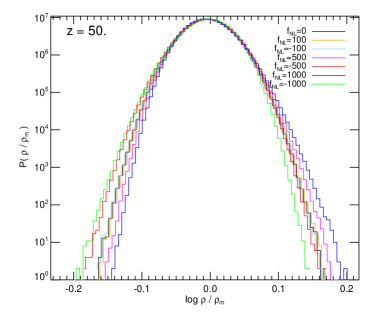
In Fig. 1 we show the probability density function of the density field, as measured in the earliest output ($z=50$) common to all our 7 simulations. It is computed on a $512^{3}$ grid, using the Triangular Shape Cloud (TSC) scheme (see, e.g. Hockney & Eastwood, 1988). From the plot it is evident that the larger the value of $f_{\rm{NL}}$, the more pronounced is the high-density tail. This reflects on the values of the skewness of the density distribution $\langle\delta^{3}\rangle$, which ranges at $z=50$ between $1.3\times 10^{-5}$ for $f_{\rm{NL}}=-1000$ and $1.4\times 10^{-4}$ for $f_{\rm{NL}}=1000$. Note that the positive values of the skewness in models with negative $f_{\rm{NL}}$ are produced by the first stages of the gravitational evolution. In fact, taking into account our sign choice in the relation between potential and density, we expect a negative (positive) skewness for the PDF when a negative (positive) $f_{\rm{NL}}$ is used. We have checked this by analyzing the simulated density field at the redshift corresponding to our initial conditions. We find that at $z_{i}$ the skewness is $-3.9\times 10^{-6}$ and $1.2\times 10^{-5}$, for $f_{\rm{NL}}=-1000$ and $f_{\rm{NL}}=1000$, respectively. The small asymmetry in the two values of the skewness is partially due to sample variance and also to the fact that the two quantities refer to different epoch since $z_{i}=96.7$ for $f_{\rm{NL}}=-1000$ and $z_{i}=100.8$ for $f_{\rm{NL}}=+1000$. The redshift evolution of the probability distribution function of density fluctuations and its moments will be discussed in detail in Sections 4.2 and 4.3.

Figure 1: The PDF for the different models (as indicated in the plot) as computed at the earliest common redshift ($z=50$).

Figure 2: Slice maps of the simulated mass density fields at $z=5.15$, $z=3.96$, $z=2.13$ and $z=0$ (rows from top to bottom). The side length is $500h^{-1}$ Mpc, while the thickness is $31.25h^{-1}$ Mpc. The panels in the middle column show the logarithm of the projected density. The left and right panels are the relative residuals for the $f_{\rm NL}$=$\pm 1000$ runs (equation [2]). Each panel has the corresponding colour bar; note that for the sake of clarity the considered ranges are different from redshift to redshift.

4 Results

In this section we investigate the evolution of the dimensionless power spectrum $\Delta^{2}(k)$, and the one-point distribution function of the mass overdensity $p(\delta,R_{s})$, focusing on its high-order moments and low-density tails.

4.1 Redshift evolution of clustering

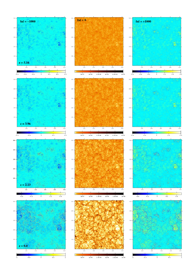
A first visual impression of how the value of $f_{\rm{NL}}$ affects the clustering evolution can be gained by looking at Fig. 2, where we show maps of the mass density field at different redshifts ranging from $z=5.16$ and $z=0$. Each slice has a side length of $500h^{-1}$ Mpc and a thickness of $31.25h^{-1}$ Mpc. The central column presents the results for the Gaussian simulation (i.e. $f_{\rm{NL}}=0$), while the relative residuals for $f_{\rm NL}=-1000$ and $f_{\rm NL}=1000$ are shown in the corresponding panels of the left and right columns. The residuals are calculated at each pixel as

$$\Delta\rho_{x}=(\rho_{x}-\rho_{0})/\rho_{0}\ ,$$ (2)

where $\rho_{x}$ represents the density for the NG map with $f_{\rm NL}=x$ and $\rho_{0}$ refers to the Gaussian field. All density fields in the plots have evolved from the same random realization of the underlying linear gravitational potential, irrespective of the statistics. For this reason, the maps of the residuals show similar features but with opposite signs.

As a first quantitative statistical test, we consider the dimensionless power spectrum $\Delta^{2}$, defined as the contribution to the variance of the fractional density per unit $\ln k$:

$$\Delta^{2}(k)\equiv\frac{d\sigma^{2}}{d\ln k}=\frac{1}{2\pi^{2}}k^{3}P(k)\ .$$ (3)

In the previous formula $P(k)$ is the matter density power spectrum.

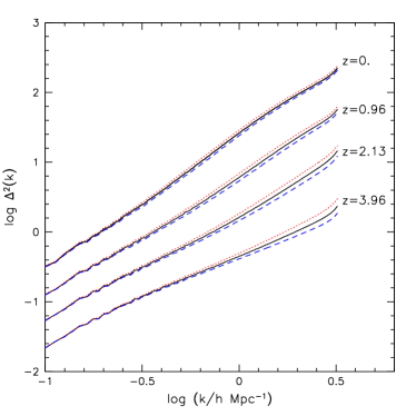
The effect of non-Gaussianity can be appreciated in Fig. 3 where we show $\Delta^{2}(k)$ computed at four different redshifts, ranging from $z=3.96$ to $z=0$. For the sake of clarity we present the results only for the scales which are in the non-linear regime (i.e. for $k>0.1$ $h$/Mpc). Moreover we show only the two most extreme NG models ($f_{\rm{NL}}=\pm 1000)$, which are compared to the Gaussian reference one.

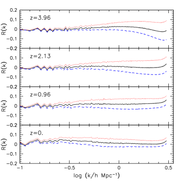
As expected, at a given redshift, a positive value of $f_{\rm{NL}}$ tends to increase the power at small scales, anticipating the formation of cosmic structures with respect to the Gaussian case. On the opposite, negative $f_{\rm{NL}}$ values delay structure formation. Fig. 3 shows that the effect is very small at $z=0$ and increases with the redshift. However, even at $z=3.96$ the largest deviations from the Gaussian case at $k=0.5$ $h$/Mpc do not exceed the 30 per cent level, i.e. well below those found in the negative tail of the PDF, as we will show in the next Section. In order to better quantify this effect, in Fig. 4 we present, for the same models and redshifts shown in Fig. 3, the logarithmic deviation, $R(k)$, of the measured $\Delta^{2}_{\rm sim}(k)$ from the analytic expression $\Delta^{2}_{\rm th}(k)$ that Smith et al. (2003) have obtained from the analysis of a large library of N-body simulations. We point out that this analytic model can be applied only to models with Gaussian initial conditions. Indeed in the simulation with $f_{\rm{NL}}=0$ we find $R(k)\equiv\log\Delta^{2}_{\rm sim}(k)-\log\Delta^{2}_{\rm th}(k)<0.01$. In the two NG models with $f_{\rm{NL}}=\pm 1000$ the dimensionless power spectrum deviates from the Gaussian case (and from the Smith et al. (2003) predictions) at $k\sim 1$ $h$/Mpc by $|R|\sim 0.04$ at $z=3.96$, $|R|\sim 0.05$ at $z=2.13$ and $z=0.96$, and $|R|\sim 0.03$ at $z=0$. Notice that at redshifts $z\ga 4$ (not shown in the plot), the differences between the dimensionless power spectra computed for the Gaussian and NG models decrease because non-linear effects on the scale of interest become negligible at large redshifts. This result suggests that the best redshift range to spot primordial non-Gaussianity is $2\la z\la 4$.

Figure 3: The redshift evolution of the dimensionless power spectrum $\Delta^{2}$. For clarity, only the non-linear scales are shown. Different lines refer to models with different primordial non-Gaussianity: $f_{\rm{NL}}=0$ (solid line), $f_{\rm{NL}}=1000$ (dotted line), $f_{\rm{NL}}=-1000$ (dashed line).

Figure 4: The logarithmic deviation $R(k)\equiv\log\Delta^{2}_{\rm sim}(k)-\log\Delta^{2}_{\rm th}(k)$ is shown for the same models and redshifts presented in Fig. 3. Here $\Delta^{2}_{\rm th}(k)$ is computed using the analytic expression of Smith et al. (2003), which is valid only for the Gaussian case.

4.2 Probability distribution function of density fluctuations

The simplest way to characterize the cosmological density field is its one-point PDF, i.e. the probability of a density fluctuation $\delta$ measured at the generic position, on a suitable smoothing scale, $R_{s}$. If the PDF of the primordial density field is Gaussian then it remains Gaussian as long as density fluctuations evolve in the linear regime. When $|\delta|\sim 1$, non-linear evolution strongly modifies the Gaussian shape of the original PDF. This picture has been confirmed by the results of different N-body simulations performed in the cold dark matter framework (see, e.g. Kayo et al., 2001, and references therein). These numerical experiments show that the evolved PDF is well approximated by a lognormal distribution:

$$P_{LN}(\delta)=\frac{1}{\sqrt{2\pi S^{2}}}\exp\left[-\frac{\left[\ln(1+\delta)+S^{2}/2\right]^{2}}{2S^{2}}\right]\frac{1}{1+\delta}\ ,$$ (4)

where the parameter $S$ is related to the variance $\sigma^{2}\equiv\langle\delta^{2}\rangle$ of the density fluctuation field: $S^{2}=\ln(1+\sigma^{2})$. The validity of this result has been thoroughly checked in the weakly non-linear regime but also seems to apply well in the non-linear regime, at least for $\sigma\la 4$ and $\delta\la 100$. This result is further corroborated by the statistical analysis of the three-dimensional distribution of galaxies (see, e.g., Croton et al., 2004; Marinoni et al., 2005). A discussion of the possible role of the lognormal distribution for cosmological structure formation can be found in Coles & Jones (1991).

Here we extend the previous analysis by investigating to what extent the lognormal model can be successfully applied to describe the evolved PDF in scenarios with primordial non-Gaussianity. To do this we have computed the mass density field of our simulations using the TSC scheme to distribute each particle mass at the points of a regular grid. To study the clustering evolution we have considered different outputs corresponding to different redshifts ($z=3.96,2.13,0.96,0$). Moreover, since the non-linear scale increases with time we have also considered two different grids: a finer one consisting of $512^{3}$ points, corresponding to a smoothing radius of $R_{s}\sim 0.98$ Mpc/h, suitable for the early stages of the evolution, and a coarser one, with $128^{3}$ points ($R_{s}\sim 3.91$ Mpc/h) for the low-redshift outputs. The PDF at the very early times ($z=50$) has been already shown in Fig. 1. It is evident that deviations from Gaussianity are very tiny even for the most extreme NG models, as quantified by the low values of the skewness.

Figure 5: The redshift evolution of the cumulative PDF of the density field smoothed on two different scales. Panels on the left: smoothing radius $R_{s}\sim 0.98$ Mpc/h. Panels on the right: smoothing radius $R_{s}\sim 3.91$ Mpc/h. The different panels refer to the four redshifts explored, indicated in the plots. Different line-styles refer to models with different primordial non-Gaussianity: $f_{\rm{NL}}=0$ (solid line), $f_{\rm{NL}}=1000$ (dotted line), $f_{\rm{NL}}=-1000$ (dashed line).

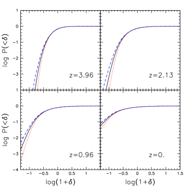
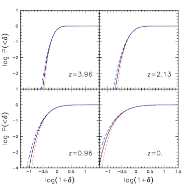
In Fig. 5 we show the cumulative PDFs at four different epochs. We prefer to show the cumulative rather than the differential PDF since, for a given overdensity threshold, the difference in the PDFs quantifies the difference in the volume occupied by structure below threshold, i.e. a quantity that can be potentially measured from real datasets. It is evident from the plots in Fig. 5 that the largest differences between models are in the low-density tail corresponding to $\log(1+\delta)\la-1$, as expected from a visual impression of Fig. 2 in which the most prominent features in the map of the residuals occur in regions that are below average density in the Gaussian case (shown in the central panels). These residuals are seen already at $z=5.16$ and their magnitude increases with time. Negative $f_{\rm{NL}}$ values increase the probability of underdense regions with respect to the Gaussian case. The opposite holds true for positive $f_{\rm{NL}}$. On the contrary, in the high-density tail, the differences between the models are much less evident. The differences are more noticeable at $z=2.13$ and decrease both at higher and lower redshifts, as already pointed out.

Finally, departures from the Gaussian case are more evident when the density field is smoothed on a small scale ($R_{s}\sim 0.98$ Mpc/h in the plots on the left hand side of Fig. 5), but can still be appreciated when smoothing on a scale of $\sim 3.91$ Mpc/h (shown in the panels on the right). Considering the density maps with $R_{s}\sim 3.91$ Mpc/h, commonly adopted in similar analyses, and an underdensity threshold $\delta=-0.9$, a value close to the mean void underdensity in numerical simulations (Colberg et al., 2008), we find that at $z=0$ only 1.3 per cent of the volume is below threshold in the Gaussian case. The difference with the NG models is striking, since the volume reduces by a factor 2.3 in the case of $f_{\rm{NL}}=1000$ and increases by $\sim 70$ per cent when $f_{\rm{NL}}=-1000$. At higher redshifts the differences further increase. With the same overdensity threshold we find that if $f_{\rm{NL}}=1000$ the volume occupied by regions with $\delta<0.9$ is a factor of $\sim 6.5$ smaller than in the Gaussian case while if $f_{\rm{NL}}=-1000$ the volume is $\sim 17$ times larger. One should note, however, that the volume fraction below this density threshold rapidly decreases with the redshift. At $z=0.9$ this fraction is only 0.007 per cent for $f_{\rm{NL}}=0$. The fact that at all redshifts departures from Gaussianity preferentially occur in low-density environments strongly suggest that dedicated statistical tests related to the void probability could be successfully applied to spot primordial non-Gaussianity. It is worth pointing out that this is a promising observational test also at the present epoch since the volume occupied by voids, in which the NG features are still well preserved, increases with time.

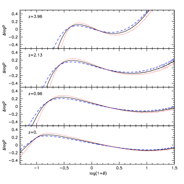
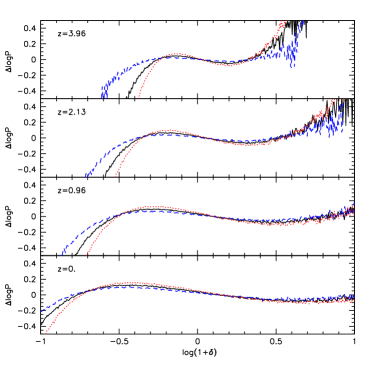
In order to check if a lognormal distribution provides a good description of the evolved PDFs even in the NG case, we compute the logarithmic deviation, $\Delta\log P\equiv\log PDF-\log P_{LN}$, where the reference lognormal $P_{LN}$ is computed from equation (4), adopting for the variance $\sigma^{2}$ the value computed directly from the N-body outputs. We notice that the value of the mass variance $\sigma^{2}$ that we measure in the Gaussian simulation agrees, at the few percent level, with the theoretical predictions of Peacock & Dodds (1996) and Smith et al. (2003), hence confirming the results of Kayo et al. (2001).

The results are displayed in Fig. 6 for the same models, redshifts and smoothing radii presented in Fig. 5. In general a lognormal distribution provides a reasonable fit to the evolved PDFs. The match is very good at intermediate overdensities ($-0.2\la\log(1+\delta)\la 0.6$) and improves when the smoothing length increases. The deviation $\Delta\log P$ increases towards both the high and the low-density tails. This trend is systematic and independent of the primordial non-Gaussianity. In particular the lognormal distribution tends to over(under)-estimate the probability of the under(over)-dense regions, and therefore cannot describe the statistical properties of both voids and highly-clustered regions. We recall that analytic theoretical predictions for the PDF, different from the lognormal model, which agree at few per cent level in the void regime have been very recently proposed by Lam & Sheth (2008).

Figure 6: The logarithmic deviation of the PDF from a lognormal distribution, $\Delta\log P$, is shown for the same models and redshifts presented in Fig. 5. Results for smoothing radii $R_{s}\sim 0.98$ and $R_{s}\sim 3.91$ Mpc/h are displayed in the left and right panels, respectively. Different lines refer to models with different primordial non-Gaussianity: $f_{\rm{NL}}=0$ (solid line), $f_{\rm{NL}}=1000$ (dotted line), $f_{\rm{NL}}=-1000$ (dashed line).

4.3 High-order moments

A way to quantify the PDF properties is to measure its high-order moments. Rigorously speaking all moments have to be specified to fully describe a distribution function. However, for practical purposes a reasonable characterization of the bulk of the PDF can be achieved using the small-order moments up to the fourth. Therefore, here we consider the second, the third and the fourth-order moments of the distribution, namely its variance $\sigma^{2}\equiv\langle\delta^{2}\rangle$, skewness $\gamma\equiv\langle\delta^{3}\rangle$ and kurtosis $\kappa\equiv\langle\delta^{4}\rangle$.

The gravity-driven clustering evolution amplifies these moments. Their growth rate, however, does not depend on the level of primordial non-Gaussianity. This is evident from Fig. 7, where we show the redshift evolution of variance, skewness and kurtosis relative to the PDF measured on the finer ($512^{3}$) grid, i.e. to a smoothing radius $R_{s}\sim 0.98$ Mpc/h. For the sake of clarity and to avoid overcrowding, we display the results for the Gaussian case ($f_{\rm{NL}}=0$) and for the two most extreme NG models ($f_{\rm{NL}}=\pm 1000$) only. The evolution of each moments is very similar in the three models, characterized by different line-styles. This is particularly evident for the variance, $\sigma^{2}$, and reflect the fact that the power spectra of the various models remain almost identical throughout the evolution. Focusing on $\gamma$ we note that NG models with positive (negative) $f_{\rm{NL}}$, characterized by a positive (negative) primordial skewness, have values of $\gamma$ that are systematically larger (smaller) than the Gaussian case by about 25 per cent . This difference, originated from the different initial conditions, is kept at the same level through the evolution history. Indeed, to a first approximation, the gravitational evolution is expected to couple high-order moments to the variance (see below), the evolution of which has only a weak dependence on $f_{\rm{NL}}$, as witnessed by the fact that the evolution of $P(k)$ depends only weakly on $f_{\rm{NL}}$ (see Section 4.1). This is also confirmed by the analysis of the other simulations of NG models with $|f_{\rm{NL}}|<1000$ (not shown). These same considerations apply to the kurtosis, $\kappa$ for which, however, deviations from the Gaussian case at $z=0$ amount to $\sim 50$ per cent.

Figure 7: The redshift evolution of variance $\sigma^{2}$, skewness $\gamma$ and kurtosis $\kappa$. Labels on the plot identifies the different moments. Different line-styles refer to models with different primordial non-Gaussianity: $f_{\rm{NL}}=0$ (solid line), $f_{\rm{NL}}=1000$ (dotted line), $f_{\rm{NL}}=-1000$ (dashed line).

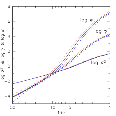
Starting from Gaussian density fluctuations, perturbation theory shows that gravitational instability leads to hierarchical scaling relations between the variance of the PDF and its higher-order moments. For this reason it is useful to repeat the previous analysis using two different quantities: the normalized skewness, defined as, $S\equiv\gamma/\sigma^{4}$ and the normalized kurtosis, $K\equiv(\kappa-3\sigma^{4})/\sigma^{6}$. Predictions of the perturbation theory by different authors have been successfully tested using N-body simulations (see, e.g., Lucchin et al., 1994, and references therein). The results, however, revealed that the values of $S$ and $K$ depend on the shape of the primordial power spectrum and on the shape and scale $R$ of the smoothing filter. For instance, with a Gaussian filter and a cold dark matter power spectrum, typical values are $S\sim 3$ and $K\sim 16$ (Kayo et al., 2001). These values also agree with the predictions of the lognormal model described by equation (4), for which (Kayo et al., 2001)

$$S(R)=3+\sigma^{2}(R)$$ (5)

and

$$K(R)=16+15\sigma^{2}(R)+6\sigma^{4}(R)+\sigma^{6}(R)\ .$$ (6)

We recall that the hierarchical scaling relations are a prediction derived under the assumption of Gaussian fluctuations. For this reason, possible deviations from the theoretical predictions have to be regarded as a signature of primordial non-Gaussianity. This is in essence the so-called skewness test suggested by Coles & Jones (1991) and Silk & Juszkiewicz (1991), according to which departures from a constant value $S$ on scales in which fluctuations are still evolving in the weakly non-linear regime provide a powerful test for NG models, as demonstrated by the analysis of first-generation NG simulations (Coles et al., 1993).

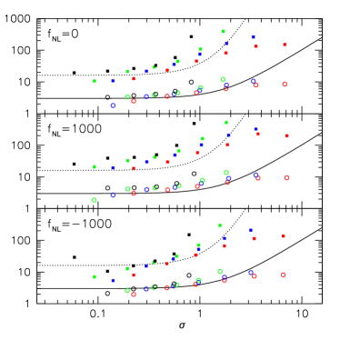
We have repeated the same test using both the normalized skewness $S$ and kurtosis $K$. The results are shown in Fig. 8 in which both quantities are shown as a function of the r.m.s. $\sigma$. The different panels refer to different numerical simulations and compare the measured $K$ (filled squares) and $S$ (open circles) with theoretical predictions of the lognormal model for which $S(R)$ and $K(R)$ are provided by equations (5) and (6) (solid and dashed curves, respectively). Each panel combines results obtained at different redshifts ($z=3.96$, $z=2.13$, $z=0.96$ and $z=0$) and using different smoothing radii ($R_{s}=(1,2,4,8,16,32)\times\Delta x$, with $\Delta x\sim 0.98$ Mpc/h). The magnitude of both moments increases with $\sigma$, independently of the value of $f_{\rm{NL}}$. Focusing on the top panel, we notice that in the low-$\sigma$ regime (i.e. $\sigma\la 1$) $S(\sigma)$ flattens but is not quite constant, which would be at variance with the predictions of the hierarchical model. However, we attribute this mismatch to a spurious effect deriving from the use of different smoothing scales. A similar trend is also seen in the two NG cases in the same low-$\sigma$ range. We conclude that, given the smallness of the effect, it is difficult to disentangle the signature of primordial non-Gaussianity from the spurious signal produced by the varying smoothing radii, hence reducing the power of the skewness test. Using the normalized kurtosis has two potential advantages. First, the signal is more than one order of magnitude larger than the normalized skewness. And second, the differences between Gaussian and NG cases in the same $\sigma$-range are significantly larger. However, as shown by Kayo et al. (2001), kurtosis has larger error than skewness. Therefore to decide which statistics is more sensitive to primordial non-Gaussianity one should perform an accurate error analysis, which is beyond the scope of this work. Such analysis would also allow to estimate and correct for systematic effects induced by the finite size of the computational box although in our case, given the large size of the computational box, the correction factor, estimated according to Kayo et al. (2001), is very small and can be safely neglected.

The plot confirms that in the weakly non-linear regime a lognormal model predicts fairly well the normalized high-order moments. Discrepancies become very significant during the non-linear evolution, i.e. when $\sigma\geq 3$ in the $S$ case and when $\sigma\geq 1$ in the $K$ case. We note that in the high-$\sigma$ regime the lognormal model systematically over-predicts the amplitude of the normalized moments in both the Gaussian and the NG models.

Figure 8: The normalized skewness $S$ (open circles) and the normalized kurtosis $K$ (filled squares) of the simulated density field as a function of $\sigma$. The corresponding theoretical values predicted by equations (5) and (6) are shown with a solid and a dashed line, respectively. Different panels refer to models with different primordial non-Gaussianity. Top: Gaussian model $f_{\rm{NL}}=0$. Middle: NG model with $f_{\rm{NL}}=+1000$ . Bottom: NG model with $f_{\rm{NL}}=-1000$ . Moments have been computed using different smoothing radii [$R_{s}=(1,2,4,8,16,32)\times\Delta x$, with $\Delta x\sim 0.98$ Mpc/h]. The colours of the symbols correspond to measurements at different redshifts: $z=3.96$ (red), $z=2.13$ (blue), $z=0.96$ (green) and $z=0$ (black).

5 Discussion and conclusions

In this work we have investigated the properties of the mass density field extracted from the N-body experiments of NG scenarios presented in Grossi et al. (2007). These models are physically motivated in the context of the inflationary theory, and cover a large range of primordial non-Gaussianity: $-1000<f_{NL}<1000$. Moreover the state-of-the art (mass, force and spatial) resolution of these simulations allows us to study the evolution of the primordial non-Gaussianity on both linear and non-linear scales, from very high redshifts to the present epoch.

Our results show that clustering properties are little affected by primordial non-Gaussianity, which is soon erased by the effect of non-linear evolution. Indeed, the power spectrum of our most extreme models matches the Gaussian case within 20-30 per cent. On the contrary, the one-point PDF of the mass density field represents a promising tool to distinguish among competing NG models. In fact, while in the high-density tail the primordial signal is quickly obliterated by non-linearly induced non-Gaussianity, in the low-density regions the primordial non-Gaussianity stands out, expecially at intermediate ($1\la z\la 2$) redshifts. The differences are preserved up to the present epoch.

This result suggests that statistics related to the void distribution could provide a powerful tool to detect primordial non-Gaussianity. Unfortunately, studying low-density environments is challenging from both a practical and a theoretical point of view. First of all, a theoretical difficulty is represented by the fact that no such statistical tool has been proposed in the context of NG models. Furthermore, even in Gaussian scenarios, there is no unique way of estimating a well-defined statistic like, for example, the void probability function. In this respect, significant progress has been recently made to define efficient and reliable void finding algorithms (see for example the comparison presented in Colberg et al., 2008, and references therein). Finally, all statistics aimed at probing low-density regions are notoriously difficult to apply because of the sparseness of the data. However, this problem might be overcome by exploiting quasar high-resolution spectra thanks to the intrinsic relation between the properties of the void in the three-dimensional mass distribution and the ”flux-voids” (defined as the connected regions in the one-dimensional flux distribution above the mean flux level; see Viel et al., 2008). We plan to investigate this issue in detail by means of dedicated, high-resolution hydrodynamical simulation of NG models.

Using spectra of distant objects to spot voids allows, in principle, to study their properties and therefore to investigate non-Gaussianity at all redshifts. At high $z$ this method will complement other statistics which are also effective in detecting NG features, like the occurrence of rare events represented by the abundance of massive clusters (see, e.g., Grossi et al., 2007), the topology of the mass distribution, that has been investigated by Hikage et al. (2008). Finally, in this paper we have studied the skewness and the kurtosis of the PDF and found that neither is very sensitive to primordial non-Gaussianity, even at very high redshifts. In this respect the bispectrum represents a much more powerful statistical tool that has been extensively used to constrain the amount of primordial non-Gaussianity in the CMB (see, e.g., Komatsu et al., 2003; Cabella et al., 2006; Spergel et al., 2007; Creminelli et al., 2007; Komatsu et al., 2008). Also, it has been successfully applied to the existing galaxy surveys at low redshift to assess the amount of non-linearity in galaxy biasing (Verde et al., 2002; Gaztañaga & Scoccimarro, 2005; Pan & Szapudi, 2005). In a future paper we plan to use our simulations to assess the power of the bispectrum in high-redshift surveys as a probe of primordial non-Gaussianity (see Sefusatti & Komatsu, 2007).

References

- Bartolo et al. (2004) Bartolo N., Komatsu E., Matarrese S., Riotto A., 2004, Phys. Rep., 402, 103
- Bartolo et al. (2005) Bartolo N., Matarrese S., Riotto A., 2005, J. Cosmology Astropart. Phys., 10, 103
- Cabella et al. (2006) Cabella P., Hansen F. K., Liguori M., Marinucci D., Matarrese S., Moscardini L., Vittorio N., 2006, MNRAS, 369, 819
- Chen (2005) Chen X., 2005, Phys. Rev. D, 72, 123518
- Colberg et al. (2008) Colberg J. M., et al., 2008, MNRAS, 387, 933
- Coles & Jones (1991) Coles P., Jones B., 1991, MNRAS, 248, 1
- Coles et al. (1993) Coles P., Moscardini L., Lucchin F., Matarrese S., Messina A., 1993, MNRAS, 264, 749
- Creminelli et al. (2007) Creminelli P., Senatore L., Zaldarriaga M., Tegmark M., 2007, J. Cosmology Astropart. Phys., 3, 5
- Croton et al. (2004) Croton D. J., et al., 2004, MNRAS, 352, 1232
- Dalal et al. (2008) Dalal N., Doré O., Huterer D., Shirokov A., 2008, Phys. Rev. D, 77, 123514
- Dunkley et al. (2008) Dunkley J., et al., 2008, preprint, astro-ph/0803.0586
- Gaztañaga & Scoccimarro (2005) Gaztañaga E., Scoccimarro R., 2005, MNRAS, 361, 824
- Grinstein & Wise (1986) Grinstein B., Wise M. B., 1986, ApJ, 310, 19
- Grossi et al. (2007) Grossi M., Dolag K., Branchini E., Matarrese S., Moscardini L., 2007, MNRAS, 382, 1261
- Hikage et al. (2008) Hikage C., Coles P., Grossi M., Moscardini L., Dolag K., Branchini E., Matarrese S., 2008, MNRAS, 385, 1613
- Hikage et al. (2006) Hikage C., Komatsu E., Matsubara T., 2006, ApJ, 653, 11
- Hockney & Eastwood (1988) Hockney R. W., Eastwood J. W., 1988, Computer simulation using particles. Bristol: Hilger, 1988
- Kang et al. (2007) Kang X., Norberg P., Silk J., 2007, MNRAS, 376, 343
- Kayo et al. (2001) Kayo I., Taruya A., Suto Y., 2001, ApJ, 561, 22
- Komatsu et al. (2003) Komatsu E., et al., 2003, ApJS, 148, 119
- Komatsu et al. (2008) Komatsu E., et al., 2008, preprint, astro-ph/0803.0547
- Lam & Sheth (2008) Lam T. Y., Sheth R. K., 2008, MNRAS, 386, 408
- Lucchin et al. (1994) Lucchin F., Matarrese S., Melott A. L., Moscardini L., 1994, ApJ, 422, 430
- Marinoni et al. (2005) Marinoni C., et al., 2005, A&A, 442, 801
- Matarrese et al. (1986) Matarrese S., Lucchin F., Bonometto S. A., 1986, ApJ, 310, L21
- Matarrese & Verde (2008) Matarrese S., Verde L., 2008, ApJ, 677, L77
- Matarrese et al. (2000) Matarrese S., Verde L., Jimenez R., 2000, ApJ, 541, 10
- Mathis et al. (2004) Mathis H., Diego J. M., Silk J., 2004, MNRAS, 353, 681
- Matsubara (2003) Matsubara T., 2003, ApJ, 584, 1
- Moscardini et al. (1991) Moscardini L., Matarrese S., Lucchin F., Messina A., 1991, MNRAS, 248, 424
- Pan & Szapudi (2005) Pan J., Szapudi I., 2005, MNRAS, 362, 1363
- Peacock & Dodds (1996) Peacock J. A., Dodds S. J., 1996, MNRAS, 280, L19
- Sefusatti & Komatsu (2007) Sefusatti E., Komatsu E., 2007, Phys. Rev. D, 76, 083004
- Shandera & Tye (2006) Shandera S. E., Tye S.-H. H., 2006, J. Cosmology Astropart. Phys., 5, 7
- Silk & Juszkiewicz (1991) Silk J., Juszkiewicz R., 1991, Nat, 353, 386
- Smith et al. (2003) Smith R. E., et al., 2003, MNRAS, 341, 1311
- Spergel et al. (2003) Spergel D. N., et al., 2003, ApJS, 148, 175
- Spergel et al. (2007) Spergel D. N., et al., 2007, ApJS, 170, 377
- Springel (2005) Springel V., 2005, MNRAS, 364, 1105
- Springel et al. (2001) Springel V., Yoshida N., White S. D. M., 2001, New Astronomy, 6, 79
- Verde et al. (2002) Verde L., et al., 2002, MNRAS, 335, 432
- Viel et al. (2008) Viel M., Colberg J. M., Kim T.-S., 2008, MNRAS, 386, 1285
- White (1994) White S. D. M., 1994, preprint, astro-ph/9410043
- Yadav & Wandelt (2008) Yadav A. P. S., Wandelt B. D., 2008, Phys. Rev. Lett., 100, 181301