Spatial characterization of the magnetic field profile of a probe tip used in magnetic resonance force microscopy

Abstract

We have developed the experimental approach to characterize spatial distribution of the magnetic field produced by cantilever tips used in magnetic resonance force microscopy (MRFM). We performed MRFM measurements on a well characterized diphenyl-picrylhydrazyl (DPPH) film and mapped the 3D field profile produced by a $Nd_{2}Fe_{14}B$ probe tip. Using our technique field profiles of arbitrarily shaped probe magnets can be imaged.

Magnetic resonance force microscopy attracted a lot of interest in the last few years due to its high force sensitivity and excellent spatial resolution of magnetic properties. MRFM has been used in studies of electron and nuclear spin systems culminating in the detection of the force signal originating from a single electron spin Rugar 2004 . Recent experiments on nuclear spins of ${}^{19}F$ in $CaF_{2}$ samples demonstrated the spatial resolution of 90 nm Mamin 2007 , orders of magnitude better than conventional magnetic resonance imaging technique. In the long term, MRFM is envisioned as a possible route to achieve imaging of individual molecules. Experiments on ferromagnetic systems showed the potential for spatially resolved ferromagnetic resonance in continuous and microfabricated samples Nazaretski 2007 ; Mewes 2006 . In MRFM experiments, force F exerted on a cantilever, is a convolution of the sample’s magnetization and the gradient of the magnetic field produced by the probe tip. To perform correct imaging, quantitative knowledge of the spatial distribution of the tip field is required. At present, the most common way to characterize magnetic tips is to use the cantilever magnetometry Rossel 1996 ; Stipe 2001 . It provides information about the magnetic moment of the tip m, however, it is also sensitive to the relative orientation of m with respect to the external magnetic field and the direction of cantilever’s oscillations. Moreover, the detailed spatial field profile of the magnetic tip can not be inferred. Alternative approach utilizes the spectroscopic nature of MRFM and has been demonstrated in previous studies Mamin 2007 ; Chao 2004 ; Wago 1998 ; Bruland 1998 ; Hammel 2003 . In these experiments the strength of the probe field has been determined from the position of the onset in the MRFM spectra as a function of the probe-sample separation $z$. Based on this information, the point dipole approximation has been used to model the magnetic tip. The situation becomes more complicated if the shape of the tip is irregular or m is tilted with respect to the $\hat{z}$ direction. Under these circumstances the one-dimensional approach is insufficient, and does not reveal the spatial field profile of the probe tip. In this letter we propose a method for detailed mapping of the tip magnetic field, free of any assumptions about the tip shape, size, or composition.
In MRFM experiments the magnetic tip of a cantilever is used to generate the inhomogeneous magnetic field causing local excitation of the spin resonance in a small volume of the sample known as sensitive slice. The resonance condition is written as follows

$$|{\bf H}_{tot}(r)|=\frac{\omega_{RF}}{\gamma},$$ (1)

where $\gamma$ is the gyromagnetic ratio. The total field ${\bf H}_{tot}(r)$ can be expressed as

$${\bf H}_{tot}(r)={\bf H}_{ext}+{\bf H}_{tip}(r),$$ (2)

where ${\bf H}_{ext}$ is the externally applied magnetic field and ${\bf H}_{tip}(r)$ is the field of the probe tip. Width $\Delta z$ of the sensitive slice is determined by the ratio of the resonance linewidth $\Delta H_{res}$ and the strength of the gradient field $\nabla H_{tip}$ produced by the probe tip, $\Delta z$ = $\frac{\Delta H}{|\nabla H_{tip}|}$ Suter 2002 . Three dimensional images of electron spin densities can be reconstructed by performing lateral and vertical scanning of the sensitive slice across the sampleWago 1998 ; Chao 2004 .

The concept behind our method for detailed characterization of the tip field profile is illustrated in Fig. 1. It requires a thin-film sample with sharp edges. When the sensitive slice touches the sample edge, a leading edge signal is detected. At this location, the sample edge is a tangent line to the sensitive slice for a reasonable magnetic tip. Thus, scanning in 3D and recording the locations corresponding to the leading edge enables full reconstruction of the sensitive slice. If desired, it can be then parameterized using dipolar, quadrupolar, etc moments.

To illustrate this procedure, we report on MRFM measurements on a well characterized DPPH film, while laterally scanning the cantilever over its edge. We used a commercially available Veeco $Si_{3}N_{4}$ cantilever with the resonance frequency of $\approx$ 8 kHz and the spring constant $k$ of $\approx$ 0.01 N/m Veeco . The original tip was removed by focused ion milling and a small magnetic particle of $Nd_{2}Fe_{14}B$ available from Magnequench Inc. Magnequench has been glued to the end of a cantilever with Stycast 1266 epoxy in the presence of an aligning magnetic field. Consequently, the tip has been magnetized in the field of 80 kOe. The MRFM tip has a spherical shape with the diameter of $\approx$ 2.4 $\mu$m and its SEM images are shown in panels (1) and (2) in Fig. 2. The saturation magnetization of $Nd_{2}Fe_{14}B$ particles has been measured in a SQUID magnetometer, and is equal to $4\pi M_{s}$ = 13 kG Nazaretski 2006a . Based on the SEM image we estimate the probe moment to be (7.5$\pm$0.4)$\times$10^-9 emu, in agreement with the value of (6.9$\pm$0.5)$\times$10^-9 emu measured by the cantilever magnetometry. The cantilever is mounted on top of a double scanning stage of a low temperature MRFM system Nazaretski 2006 ; Attocube . For data acquisition, the temperature was stabilized at 10 K and the amplitude modulation scheme has been implemented to couple to the in-resonance spins. The DPPH powder DPPH was dissolved in acetone and deposited on a 100 $\mu$m thick silicon wafer in a spin-coater at 3000 rpm. To protect the film, 20 nm of Ti was deposited on top of DPPH. Approximately 2$\times$1.6 mm² piece was cleaved from a wafer and glued to the strip-line resonator of the microscope. The structure of the film and sharpness of edges were inspected in SEM and are shown in Fig. 2. The film was found to be continuous, and its thickness varied between 400 and 600 nm.

Fig. 3 shows the typical MRFM spectrum recorded in a DPPH film. When the tip is located above the film, the strongest tip field experienced by the sample is situated directly under the probe magnet (assuming ${\bf m}$ $\parallel$ ${\bf H}_{ext}$). The field value in the MRFM spectrum where the sensitive slice just touches the DPPH film is called the leading edge Suter 2002 , and is indicated by arrows in Fig. 3.

The large positive peak at $\approx$ 3.34 kOe corresponds to the bulk-like resonance. It originates from the large region of the sample where the tip field is small, but due to the large number of spins the MRFM signal is significant. The field difference between the bulk-like resonance and the position of the leading edge provides the direct measure of the probe field strength.

Fig. 1 shows the schematic of the characterization experiment. We fixed the probe-sample separation $z$, and approached different edges of the DPPH film while tracking the leading edge. The left panel of Fig. 4 shows the field evolution of the leading edge for two values of $z$ and three different directions of lateral scanning over the film edge. The almost identical shape of the curves indicates that m is approximately parallel to the direction of ${\bf H}_{ext}$. In the first approximation, our tip can be modeled as a magnetic dipole. The field profile produced on the surface of the sample can be written as follows Jackson 1975 :

$$H(R,\theta,\varphi) =\frac{4\pi M_{s}r_{0}^{3}}{3}\times\{\frac{-3z(\sin\theta(x\sin\varphi+y\cos\varphi))}{R^{5}}+$$ (3)

$$+\frac{3z^{2}\cos\theta}{R^{5}}-\frac{\cos\theta}{R^{3}}\},$$

where $4\pi M_{s}$ is the saturation magnetization of $Nd_{2}Fe_{14}B$, $r_{0}$ is the radius of the tip, $R$ is the vector to the point where the field is determined, $\theta$ and $\varphi$ are the angles which describe the spatial orientation of m (see Fig. 1).
The right panel of Fig. 4 shows the z-component of the probe field on the sample’s surface as a function of $z$. Solid line is the fit using Eq. 3 and assuming parallel orientation of m and ${\bf H}_{ext}$. Fig. 5(a) shows the comparison between the lateral field profile of the tip simulated according to Eq. 3, and the actual data points taken from the left panel of Fig. 4. Good agreement between the observed and expected behavior suggests that, indeed, our probe tip can be approximated as a dipole, and its magnetization is aligned along the direction of ${\bf H}_{ext}$. In case of any significant misalignment the tip field profile would change substantially, as shown in Fig. 5(a). For both simulations shown in Fig. 4 and 5, we had to offset the probe-sample separation by 1.42 $\pm$ 0.03 $\mu$m ($z$ is the only free parameter in the fit) which suggests that due to the short range probe-sample interaction the cantilever snaps to the sample at distances smaller than 1.42 $\mu$m Berger 1999 ; Dorofeyev 1999 . The presence of an offset may indicate the reduced magnetic moment of the tip. However, our cantilever magnetometry measurements of the tip moment agree well with the expected value, as mentioned earlier in the paper. Moreover, in Fig. 5(b) we show the calculated spatial field profile of 2 $\mu$m, 2.2 $\mu$m and 2.4 $\mu$m diameter tips. The fit for the 2.4 $\mu$m diameter tip provides the best agreement with the data points. Another argument in support of our tip model pertains to the magnitude of the MRFM force exerted on a cantilever in a particular sensitive slice. In Fig. 3 we take the measured MRFM force at $H_{ext}$ = 3.038 kOe and compare it to our estimates. The calculations yield the force value of $\approx$ 6.9$\times$10^-13 N in good agreement with the measured value of 5.7$\times$10^-13 N. Thus, dipolar approximation and our assumptions for the tip moment were adequate for the present experiment. Importantly, the same technique could be applied to map field profile from a more irregular tip.

In summary, we have studied the evolution of locally excited electron-spin resonance in a DPPH film. By tracking the position of the leading edge in MRFM spectra for different hight and direction of the approach to the sample, we have determined the spatial field profile of the cantilever tip. Measuring the MRFM signal onset over the large range of positions with adequate sensitivity allows to deconvolve the spatial field profile produced by arbitrarily shaped magnetic tips used in the magnetic resonance force microscopy.

This work was supported by the US Department of Energy and was performed, in part, at the Center for Integrated Nanotechnologies at Los Alamos and Sandia National Laboratories. Personnel at Ohio State University was supported by the US Department of Energy through grant DE-FG02-03ER46054.

Figure Caption

FIG.1 Schematic of the tip characterization technique. Detection of the leading edge signal indicates that the sample edge is tangent to the sensitive slice. 3D scanning can thus be used to fully reconstruct the shape of the sensitive slice.

FIG.2 Panel (1)and (2): SEM images of the probe magnet. Panel (3) shows the edge of the DPPH film and panel (4) is the top view showing fine structures on the surface of the film.

FIG.3 Amplitude and phase of the MRFM signal recorded at $T$ = 10 K, $\omega_{RF}$ = 9.35 GHz, $z$ = 0.73 $\mu$m. The position of the leading edge is indicated by arrows.

FIG.4 Left panel: field evolution of the leading edge as a function of lateral position over the DPPH film edge. The upper and lower set of curves correspond to $z$ = 2.35 $\mu$m and $z$ = 0.53 $\mu$m respectively. Circles represent the approach of the sample from side ’1’, squares from side ’2’ and triangles form side ’3’ of the sample as shown in Fig. 1. Right panel: the $z$-component of the tip field as a function of the probe-sample separation (left Y-axis) and the corresponding field gradient (right Y-axis). Solid curve is the fit to Eq. 3.

FIG.5 (a) Lateral field profile of the tip for approaches of sides ’1’ and ’3’ of the sample, as shown in Fig. 1. Data points are taken from the left panel in Fig. 4. ’0’ on the X-axis corresponds to the edge of the film. Upper and lower data points correspond to $z$ = 0.53 $\mu$m and $z$ = 2.35 $\mu$m respectively. Solid curve is fitted to the data using Eq. 3. Dotted and dashed lines show the expected field profile of the tip where $\theta$ = $\varphi$ = 20^∘ and $\theta$ = -20^∘, $\varphi$ = 20^∘ respectively. (b) expected field profile for the tip with $r_{0}$=1.2 $\mu$m, z-offset=1.4 $\mu$m (solid line), $r_{0}$=1.1 $\mu$m, z-offset=1.12 $\mu$m (dotted line) and $r_{0}$=1.0 $\mu$m, z-offset=0.85 $\mu$m (dashed line).

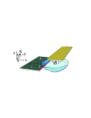
Figure 1:

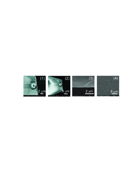
Figure 2:

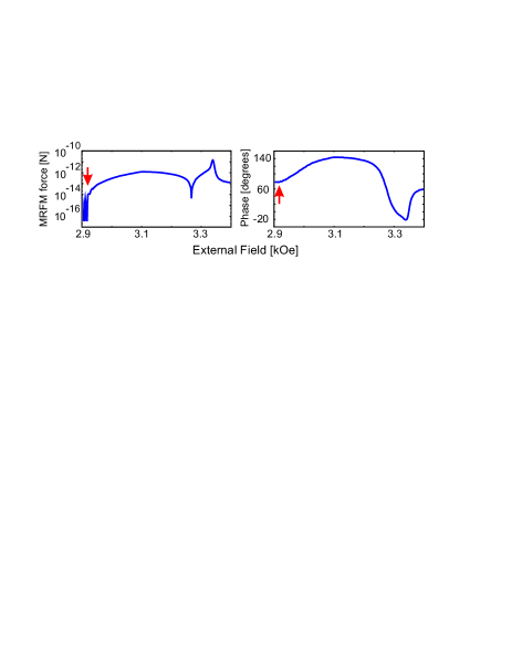
Figure 3:

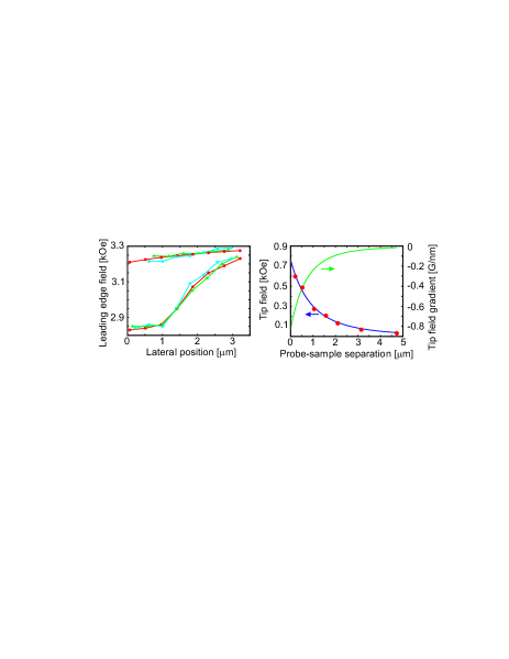
Figure 4:

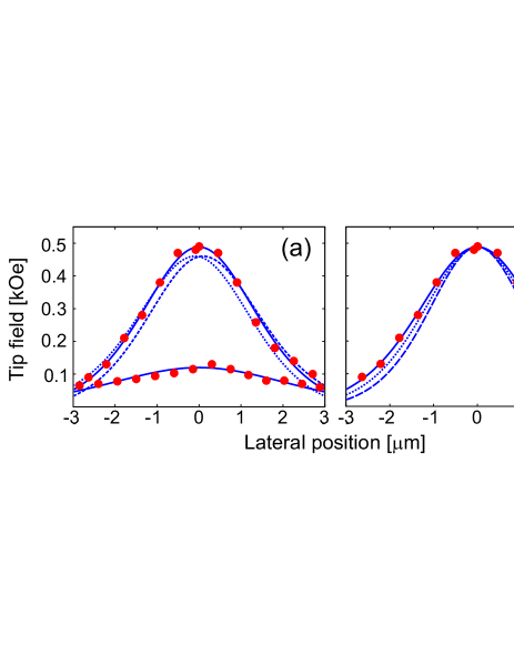
Figure 5:

References

- (1) D. Rugar, R. Budakian, H. J. Mamin, and W. Chui, Nature 430, 329 (2004)
- (2) H.J. Mamin, M. Poggio, C. L. Degen, D. Rugar, Nature Nanotech. 2, 301 (2007)
- (3) E. Nazaretski, D. V. Pelekhov, I. Martin, M. Zalalutdinov, J. W. Baldwin, T. Mewes, B. Houston, P. C. Hammel, and R. Movshovich, Appl. Phys. Lett. 90 234105 (2007)
- (4) T. Mewes, J. Kim, D. V. Pelekhov, G. N. Kakazei, P. E. Wigen, S. Batra, and P. C. Hammel, Phys. Rev. B 74, 144424 (2006)
- (5) S. Chao, W. M. Dougherty, J. L. Garbini and J. A. Sidles, Rev. Sci. Inst. 75, 1175 (2004)
- (6) K. Wago, D. Botkin, C. S. Yannoni, and D. Rugar, Appl. Phys. Lett. 72, 2757 (1998)
- (7) K. J. Bruland, W. M. Dougherty, J. L. Garbini, J. A. Sidles, and S. H. Chao, Appl. Phys. Lett. 73, 3159 (1998)
- (8) P. C. Hammel, D. V. Pelekhov, P. E. Wigen, T. R. Gosnell, M. M. Mizdor, and M. L. Roukes, Proceedings of IEEE, 91 789 (2003)
- (9) C. Rossel, P. Bauer, D. Zech, J. Hofer, M. Willemin, and H. Keller, J. Appl. Phys., 79 8166 (1996)
- (10) B. C. Stipe, H. J. Mamin, T. D. Stowe, T. W. Kenny, and D. Rugar, Phys. Rev. Lett. 86, 2874 (2001)
- (11) B. C. Stipe, H. J. Mamin, C. S. Yannoni, T. D. Stowe, T. W. Kenny, and D. Rugar, Phys. Rev. Lett. 87, 277602 (2001)
- (12) Veeco Probes, type MLCT-NO, cantilever C
- (13) http://www.magnequench.com/
- (14) Staveley Sensors piezotube is mounted on top of an Attocube 3D positioner ANPxyz100/LIN/LT/HV equipped with the optical position redout.
- (15) E. Nazaretski, J. D. Thompson, M. Zalalutdinov, J. W. Baldwin, B. Houston, T. Mewes, D. V. Pelekhov, P. Wigen, P. C. Hammel, and R. Movshovich, J. Appl. Phys. 101, 074905 (2007)
- (16) E. Nazaretski, T. Mewes, D. Pelekhov, P. C. Hammel, and R. Movshovich, AIP Conf. Proc. 850, 1641 (2006)
- (17) Sigma Chemical Co. (St. Louis, USA)
- (18) A. Suter, D. Pelekhov, M. Roukes, and P. C. Hammel, J. Magn. Res., 154, 210 (2002)
- (19) J. D. Jackson Classical Electrodynamics 3rd edition, Wiley, New York, 1999
- (20) M. Saint Jean, S. Hudlet, C. Guthmann, and J. Berger, J. Appl. Phys. 86, 5245 (1999)
- (21) I. Dorofeyev, H. Fuchs, G. Wenning, and B. Gotsmann, Phys. Rev. Lett. 83, 2402 (1999)