Asymptotically Good LDPC Convolutional Codes Based on Protographs

Abstract

LDPC convolutional codes have been shown to be capable of achieving the same capacity-approaching performance as LDPC block codes with iterative message-passing decoding. In this paper, asymptotic methods are used to calculate a lower bound on the free distance for several ensembles of asymptotically good protograph-based LDPC convolutional codes. Further, we show that the free distance to constraint length ratio of the LDPC convolutional codes exceeds the minimum distance to block length ratio of corresponding LDPC block codes.

I Introduction

Along with turbo codes, low-density parity-check (LDPC) block codes form a class of codes which approach the (theoretical) Shannon limit. LDPC codes were first introduced in the $1960$s by Gallager [1]. However, they were considered impractical at that time and very little related work was done until Tanner provided a graphical interpretation of the parity-check matrix in 1981 [2]. More recently, in his Ph.D. Thesis, Wiberg revived interest in LDPC codes and further developed the relation between Tanner graphs and iterative decoding [3].

The convolutional counterpart of LDPC block codes was introduced in [4], and LDPC convolutional codes have been shown to have certain advantages compared to LDPC block codes of the same complexity [5, 6]. In this paper, we use ensembles of tail-biting LDPC convolutional codes derived from a protograph-based ensemble of LDPC block codes to obtain a lower bound on the free distance of unterminated, asymptotically good, periodically time-varying LDPC convolutional code ensembles, i.e., ensembles that have the property of free distance growing linearly with constraint length.

In the process, we show that the minimum distances of ensembles of tail-biting LDPC convolutional codes (introduced in [7]) approach the free distance of an associated unterminated, periodically time-varying LDPC convolutional code ensemble as the block length of the tail-biting ensemble increases. We also show that, for protographs with regular degree distributions, the free distance bounds are consistent with those recently derived for regular LDPC convolutional code ensembles in [8] and [9]. Further, for protographs with irregular degree distributions, we obtain new free distance bounds that grow linearly with constraint length and whose free distance to constraint length ratio exceeds the minimum distance to block length ratio of the corresponding block codes.

The paper is structured as follows. In Section II, we briefly introduce LDPC convolutional codes. Section III summarizes the technique proposed by Divsalar to analyze the asymptotic distance growth behavior of protograph-based LDPC block codes [10]. In Section IV, we describe the construction of tail-biting LDPC convolutional codes as well as the corresponding unterminated, periodically time-varying LDPC convolutional codes. We then show that the free distance of a periodically time-varying LDPC convolutional code is lower bounded by the minimum distance of the block code formed by terminating it as a tail-biting LDPC convolutional code. Finally, in Section V we present new results on the free distance of ensembles of LDPC convolutional codes based on protographs.

II LDPC convolutional codes

We start with a brief definition of a rate $R=b/c$ binary LDPC convolutional code $\mathcal{C}$. (A more detailed description can be found in [4].) A code sequence $\mathbf{v}_{[0,\infty]}$ satisfies the equation

$$\mathbf{v}_{[0,\infty]}\mathbf{H}_{[0,\infty]}^{\mathtt{T}}=\mathbf{0},$$ (1)

where $\mathbf{H}_{[0,\infty]}^{\mathtt{T}}$ is the syndrome former matrix and

$\mathbf{H}_{[0,\infty]}=$
$\left[\begin{array}[]{cccccc}\mathbf{H}_{0}(0)&&&&\\ \mathbf{H}_{1}(1)&\mathbf{H}_{0}(1)&&&\\ \vdots&\vdots&&\ddots&\\ \mathbf{H}_{m_{\text{s}}}(m_{\text{s}})&\mathbf{H}_{m_{\text{s}}-1}(m_{\text{s}})&\ldots&\mathbf{H}_{0}(m_{\text{s}})&\\ &\mathbf{H}_{m_{\text{s}}}(m_{\text{s}}+1)&\mathbf{H}_{m_{\text{s}}-1}(m_{\text{s}}+1)&\ldots&\mathbf{H}_{0}(m_{\text{s}}+1)\\ &\ddots&\ddots&&\ddots\end{array}\right]$

is the parity-check matrix of the convolutional code $\mathcal{C}$. The submatrices $\mathbf{H}_{i}(t)$, $i=0,1,\cdots,m_{\text{s}}$, $t\geq 0$, are binary $\left(c-b\right)\times c$ submatrices, given by

$$\mathbf{H}_{i}(t)=\left[\begin{array}[]{ccc}h_{i}^{(1,1)}(t)&\cdots&h_{i}^{(1,c)}(t)\\ \vdots&&\vdots\\ h_{i}^{(c-b,1)}(t)&\cdots&h_{i}^{(c-b,c)}(t)\\ \end{array}\right],$$ (2)

that satisfy the following properties:

1. $\mathbf{H}_{i}(t)=\mathbf{0},~{}i<0$ and $i>m_{s},~{}\forall~{}t.$

2. There is a $t$ such that $\mathbf{H}_{m_{\text{s}}}(t)\neq\mathbf{0}.$

3. $\mathbf{H}_{0}(t)\neq\mathbf{0}$ and has full rank $\forall\,\,t$.

We call $m_{\text{s}}$ the syndrome former memory and $\nu_{\text{s}}=(m_{\text{s}}+1)\cdot c$ the decoding constraint length. These parameters determine the width of the nonzero diagonal region of $\mathbf{H}_{[0,\infty]}.$ The sparsity of the parity-check matrix is ensured by demanding that its rows have very low Hamming weight, i.e., $w_{H}(\mathbf{h}_{i})<<(m_{\text{s}}+1)\cdot c,~{}i>0$, where $\mathbf{h}_{i}$ denotes the $i$-th row of $\mathbf{H}_{[0,\infty]}$. The code is said to be regular if its parity-check matrix $\mathbf{H}_{[0,\infty]}$ has exactly $J$ ones in every column and, starting from row $(c-b)m_{\text{s}}+1$, $K$ ones in every row. The other entries are zeros. We refer to a code with these properties as an $(m_{\text{s}},J,K)$-regular LDPC convolutional code, and we note that, in general, the code is time-varying and has rate $R=1-J/K$. An $(m_{\text{s}},J,K)$-regular time-varying LDPC convolutional code is periodic with period $T$ if $\mathbf{H}_{i}(t)$ is periodic, i.e., $\mathbf{H}_{i}(t)=\mathbf{H}_{i}(t+T),\forall~{}i,t$, and if $\mathbf{H}_{i}(t)=\mathbf{H}_{i},\forall~{}i,t$, the code is time-invariant.

An LDPC convolutional code is called irregular if its row and column weights are not constant. The notion of degree distribution is used to characterize the variations of check and variable node degrees in the Tanner graph corresponding to an LDPC convolutional code. Optimized degree distributions have been used to design LDPC convolutional codes with good iterative decoding performance in the literature (see, e.g., [7, 11, 12, 13]), but no distance bounds for irregular LDPC convolutional code ensembles have been previously published.

III Protograph Weight Enumerators

Suppose a given protograph has $n_{v}$ variable nodes and $n_{c}$ check nodes. An ensemble of protograph-based LDPC block codes can be created by the copy-and-permute operation [14]. The Tanner graph obtained for one member of an ensemble created using this method is illustrated in Fig. 1.

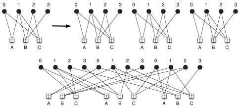
Figure 1: The copy-and-permute operation for a protograph.

The parity-check matrix $H$ corresponding to the ensemble of protograph-based LDPC block codes can be obtained by replacing ones with $N\times N$ permutation matrices and zeros with $N\times N$ all zero matrices in the underlying protograph parity-check matrix $P$, where the permutation matrices are chosen randomly and independently. The protograph parity-check matrix $P$ corresponding to the protograph given in Figure 1 can be written as

,

where we note that, since the row and column weights of $P$ are not constant, $P$ represents the parity-check matrix of an irregular LDPC code. If a variable node and a check node in the protograph are connected by $r$ parallel edges, then the associated entry in $P$ equals $r$ and the corresponding block of $H$ consists of a summation of $r$ $N\times N$ permutation matrices. The sparsity condition of an LDPC parity-check matrix is thus satisfied for large $N$. The code created by applying the copy-and-permute operation to an $n_{c}\times n_{v}$ protograph parity-check matrix $P$ has block length $n=Nn_{v}$. In addition, the code has the same rate and degree distribution for each of its variable and check nodes as the underlying protograph code.

Combinatorial methods of calculating ensemble average weight enumerators have been presented in [10] and [15]. The remainder of this Section summarizes the methods presented in [10].

III-A Ensemble weight enumerators

Suppose a protograph contains $m$ variable nodes to be transmitted over the channel and $n_{v}-m$ punctured variable nodes. Also, suppose that each of the $m$ transmitted variable nodes has an associated weight $d_{i}$, where $0\leq d_{i}\leq N$ for all $i$. Let $S_{d}=\{(d_{1},d_{2},\ldots,d_{m})\}$ be the set of all possible weight distributions such that $d_{1}+\ldots+d_{m}=d$, and let $S_{p}$ be the set of all possible weight distributions for the remaining punctured nodes. The ensemble weight enumerator for the protograph is then given by

$$A_{d}=\sum_{\{d_{k}\}\in S_{d}}\sum_{\{d_{j}\}\in S_{p}}A_{\mathbf{d}},$$ (3)

where $A_{\mathbf{d}}$ is the average number of codewords in the ensemble with a particular weight distribution $\textbf{d}=(d_{1},d_{2},\ldots,d_{n_{v}})$.

III-B Asymptotic weight enumerators

The normalized logarithmic asymptotic weight distribution of a code ensemble can be written as $r(\delta)=\lim_{n\rightarrow\infty}\textrm{sup }r_{n}(\delta),$ where $r_{n}(\delta)=\frac{\textrm{ln}(A_{d})}{n}$, $\delta=d/n$, $d$ is the Hamming distance, $n$ is the block length, and $A_{d}$ is the ensemble average weight distribution.

Suppose the first zero crossing of $r(\delta)$ occurs at $\delta=\delta_{min}$. If $r(\delta)$ is negative in the range $0<\delta<\delta_{min}$, then $\delta_{min}$ is called the minimum distance growth rate of the code ensemble. By considering the probability

$$\mathbb{P}(d<\delta_{min}n)=\sum^{\delta_{min}n-1}_{d=1}A_{d},$$

it is clear that, as the block length $n$ grows, if $\mathbb{P}(d<\delta_{min}n)<<1$, then we can say with high probability that the majority of codes in the ensemble have a minimum distance that grows linearly with $n$ and that the distance growth rate is $\delta_{min}$.

IV Free distance bounds

In this section we present a method for obtaining a lower bound on the free distance of an ensemble of unterminated, asymptotically good, periodically time-varying LDPC convolutional codes derived from protograph-based LDPC block codes. To proceed, we will make use of a family of tail-biting LDPC convolutional codes with incremental increases in block length. The tail-biting codes will be used as a tool to obtain the desired bound on the free distance of the unterminated codes.

IV-A Tail-biting convolutional codes

Suppose that we have an $n_{c}\times n_{v}$ protograph parity-check matrix $P$, where gcd$(n_{c},n_{v})=y$. We then partition $P$ as a $y\times y$ block matrix as follows:

$$P=\left[\begin{array}[]{ccc}P_{1,1}&\ldots&P_{1,y}\\ \vdots&&\vdots\\ P_{y,1}&\ldots&P_{y,y}\end{array}\right],$$

where each block $P_{i,j}$ is of size $n_{c}/y\times n_{v}/y$. $P$ can thus be separated into a lower triangular part, $P_{l}$, and an upper triangular part minus the leading diagonal, $P_{u}$. Explicitly,

$P_{l}=\left[\begin{array}[]{cccc}P_{1,1}&&\\ P_{2,1}&P_{2,2}&&\\ \vdots&\vdots&\ddots&\\ P_{y,1}&P_{y,2}&\ldots&P_{y,y}\end{array}\right]\textrm{ and }P_{u}=\left[\begin{array}[]{cccc}&P_{1,2}&\ldots&P_{1,y}\\ &&\ddots&\vdots\\ &&&P_{y-1,y}\\ &&&\end{array}\right]$,

where blank spaces correspond to zeros. This operation is called ‘cutting’ a protograph parity-check matrix.

Rearranging the positions of these two triangular matrices and repeating them indefinitely results in a parity-check matrix $H_{cc}$ of an unterminated, periodically time-varying convolutional code with constraint length $\nu_{\text{s}}=n_{v}$ and period $T=y$ given by

$$H_{\textrm{cc}}=\left[\begin{array}[]{cccc}P_{l}&&&\\ P_{u}&P_{l}&&\\ &P_{u}&P_{l}&\\ &&\ddots&\ddots\end{array}\right].$$ (4)

Note that if gcd$(n_{c},n_{v})=1$, we cannot form a square block matrix larger than $1\times 1$ with equal size blocks. In this case, $P_{l}=P$ and $P_{u}$ is the all zero matrix of size $n_{c}\times n_{v}$. This trivial cut results in a convolutional code with syndrome former memory zero, with repeating blocks of the original protograph on the leading diagonal. It is necessary in this case to create a larger protograph parity-check matrix by using the copy and permute operation on $P$. This results in an $Mn_{c}\times Mn_{v}=n_{c}^{\prime}\times n_{v}^{\prime}$ parity-check matrix for some small integer $M$. The $n_{c}^{\prime}\times n_{v}^{\prime}$ protograph parity-check matrix can then be cut following the procedure outlined above. In effect, the choice of $M\times M$ permutation matrix creates a mini ensemble of block codes suitable to be unwrapped to an ensemble of convolutional codes.

We now introduce the notion of tail-biting convolutional codes by defining an ‘unwrapping factor’ $\lambda$ as the number of times the sliding convolutional structure is repeated. For $\lambda>1$, the parity-check matrix $H_{\textrm{tb}}^{(\lambda)}$ of the desired tail-biting convolutional code can be written as

$$H_{\textrm{tb}}^{(\lambda)}=\left[\begin{array}[]{ccccc}P_{l}&&&&P_{u}\\ P_{u}&P_{l}&&&\\ &P_{u}&P_{l}&&\\ &&\ddots&\ddots&\\ &&&P_{u}&P_{l}\end{array}\right]_{\lambda n_{c}\times\lambda n_{v}}.$$

Note that the tail-biting convolutional code for $\lambda=1$ is simply the original block code.

IV-B A tail-biting LDPC convolutional code ensemble

Given a protograph parity-check matrix $P$, we generate a family of tail-biting convolutional codes with increasing block lengths $\lambda n_{v}$, $\lambda=1,2,\ldots$, using the process described above. Since tail-biting convolutional codes are themselves block codes, we can treat the Tanner graph of $H_{\textrm{tb}}^{(\lambda)}$ as a protograph for each value of $\lambda$. Replacing the entries of this matrix with either $N\times N$ permutation matrices or $N\times N$ all zero matrices, as discussed in Section III, creates an ensemble of LDPC codes that can be analyzed asymptotically as $N$ goes to infinity, where the sparsity condition of an LDPC code is satisfied for large $N$. Each tail-biting LDPC code ensemble, in turn, can be unwrapped and repeated indefinitely to form an ensemble of unterminated, periodically time-varying LDPC convolutional codes with constraint length $\nu_{s}=Nn_{v}$ and, in general, period $T=\lambda y$.

Intuitively, as $\lambda$ increases, the tail-biting code becomes a better representation of the associated unterminated convolutional code, with $\lambda\rightarrow\infty$ corresponding to the unterminated convolutional code itself. This is reflected in the weight enumerators, and it is shown in Section V that increasing $\lambda$ provides us with distance growth rates that converge to a lower bound on the free distance growth rate of the unterminated convolutional code.

IV-C A free distance bound

Tail-biting convolutional codes can be used to establish a lower bound on the free distance of an associated unterminated, periodically time-varying convolutional code by showing that the free distance of the unterminated code is lower bounded by the minimum distance of any of its tail-biting versions. A proof can be found in [9].

Theorem 1

Consider a rate $R=(n_{v}-n_{c})/n_{v}$ unterminated, periodically time-varying convolutional code with decoding constraint length $\nu_{\text{s}}=Nn_{v}$ and period $T=\lambda y$. Let $d_{min}$ be the minimum distance of the associated tail-biting convolutional code with length $n=\lambda Nn_{v}$ and unwrapping factor $\lambda>0$. Then the free distance $d_{free}$ of the unterminated convolutional code is lower bounded by $d_{min}$ for any unwrapping factor $\lambda$, i.e.,

$$d_{free}\geq d_{min},\quad\forall\lambda>0.$$ (5)

A trivial corollary of the above theorem is that the minimum distance of a protograph-based LDPC block code is a lower bound on the free distance of the associated unterminated, periodically time-varying LDPC convolutional code. This can be observed by setting $\lambda=1$.

IV-D The free distance growth rate

One must be careful in comparing the distance growth rates of codes with different underlying structures. A fair basis for comparison generally requires equating the complexity of encoding and/or decoding of the two codes. Traditionally, the minimum distance growth rate of block codes is measured relative to block length, whereas constraint length is used to measure the free distance growth rate of convolutional codes. These measures are based on the complexity of decoding both types of codes on a trellis. Indeed, the typical number of states required to decode a block code on a trellis is exponential in the block length, and similarly the number of states required to decode a convolutional code is exponential in the constraint length. This has been an accepted basis of comparing block and convolutional codes for decades, since maximum-likelihood decoding can be implemented on a trellis for both types of codes.

The definition of decoding complexity is different, however, for LDPC codes. The sparsity of their parity-check matrices, along with the iterative message-passing decoding algorithm typically employed, implies that the decoding complexity per symbol depends on the degree distribution of the variable and check nodes and is independent of both the block length and the constraint length. The cutting technique we described in Section IV-A preserves the degree distribution of the underlying LDPC block code, and thus the decoding complexity per symbol is the same for the block and convolutional codes considered in this paper.

Also, for randomly constructed LDPC block codes, state-of-the-art encoding algorithms require only $O(g)$ operations per symbol, where $g<<n$ [16], whereas for LDPC convolutional codes, if the parity-check matrix satisfies the conditions listed in Section II, the number of encoding operations per symbol is only $O(1)$ [17]. Here again, the encoding complexity per symbol is essentially independent of both the block length and the constraint length.

Hence, to compare the distance growth rates of LDPC block and convolutional codes, we consider the hardware complexity of implementing the encoding and decoding operations in hardware. Typical hardware storage requirements for both LDPC block encoders and decoders are proportional to the block length $n$. The corresponding hardware storage requirements for LDPC convolutional encoders and decoders are proportional to the decoding constraint length [17].

V Results and Discussion

V-A Distance growth rate results

We now present distance growth rate results for several ensembles of rate $1/2$ asymptotically good LDPC convolutional codes based on protographs.

Example $1$ Consider a $(3,6)$ regular LDPC code with the folowing protograph:

.

For this example, the minimum distance growth rate is $\delta_{min}=0.023$, as originally calculated by Gallager [1]. A family of tail-biting LDPC convolutional code ensembles can be generated according to the following cut:

.

For each $\lambda$, the minimum distance growth rate $\delta_{min}$ was calculated for the tail-biting LDPC convolutional codes using the approach outlined in Section IV-B. The distance growth rates for each $\lambda$ are given as

$$\delta_{min}=\frac{d_{min}}{n}=\frac{d_{min}}{\lambda Nn_{v}}=\frac{d_{min}}{\lambda\nu_{\text{s}}}.$$ (6)

The free distance growth rate of the associated rate $1/2$ ensemble of unterminated, periodically time-varying LDPC convolutional codes is $\delta_{free}=d_{free}/\nu_{\text{s}}$, as discussed above. Then (5) gives us the lower bound

$$\delta_{free}=\frac{d_{free}}{\nu_{\text{s}}}\geq\frac{d_{min}}{\nu_{\text{s}}}=\lambda\delta_{min}$$ (7)

for $\lambda\geq 1$. These growth rates are plotted in Fig. 2.

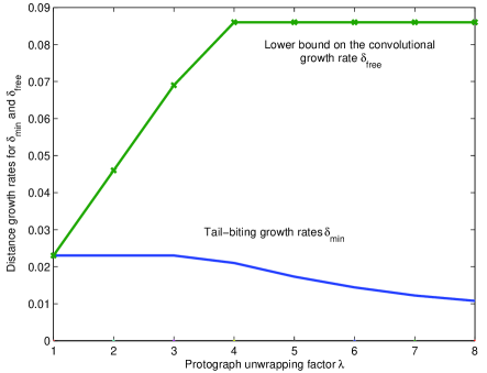
Figure 2: Distance growth rates for Example $1$.

We observe that, once the unwrapping factor $\lambda$ of the tail-biting convolutional codes exceeds $3$, the lower bound on $\delta_{free}$ levels off at $\delta_{free}\geq 0.086$, which agrees with the results presented in [8] and [9] and represents a significant increase over the value of $\delta_{min}$. In this case, the minimum weight codeword in the unterminated convolutional code also appears as a codeword in the tail-biting code.

Example $2$ The following irregular protograph is from the Repeat Jagged Accumulate [19] (RJA) family. It was shown to have a good iterative decoding threshold ($\gamma_{\textrm{iter}}=1.0$ dB) while maintaining linear minimum distance growth ($\delta_{min}=0.013$). We display below the associated $P$ matrix and cut used to generate the family of tail-biting LDPC convolutional code ensembles.

$\leftrightsquigarrow$ .

We observe that, as in Example $1$, the minimum distance growth rates calculated for increasing $\lambda$ provide us with a lower bound on the free distance growth rate of the convolutional code ensemble using (7). The lower bound was calculated as $\delta_{free}\geq 0.057$ (for $\lambda\geq 5$), significantly larger than the minimum distance growth rate $\delta_{min}$ of the underlying block code ensemble.

Example $3$ The following irregular protograph is from the Accumulate Repeat Jagged Accumulate family (ARJA) [19]:

,

where the undarkened circle represents a punctured variable node. This protograph is of significant practical interest, since it was shown to have $\delta_{min}=0.015$ and iterative decoding threshold $\gamma_{\textrm{iter}}=0.628$, i.e., pre-coding the protograph of Example $2$ provides an improvement in both values.

In this ARJA example, the protograph matrix $P$ is of size $n_{c}\times n_{v}=3\times 5$. We observe that gcd$(n_{c},n_{v})=1$, and thus we have the trivial cut mentioned in Section IV-A. We must then copy and permute $P$ to generate a mini ensemble of block codes. Results are shown for one particular member of the mini ensemble with $M=2$, but a change in performance can be obtained by varying the particular permutation chosen. Increasing $\lambda$ for the chosen permutation results in a lower bound, found using (7), of $\delta_{free}\geq 0.053$ for $\lambda\geq 4$. Again, we observe a significant increase in $\delta_{free}$ compared to $\delta_{min}$.

V-B Simulation results

Simulation results for LDPC block and convolutional codes based on the protograph of Example $3$ were obtained assuming BPSK modulation and an additive white Gaussian noise channel (AWGNC). All decoders were allowed a maximum of $100$ iterations, and the block code decoders employed a syndrome-check based stopping rule. As a result of their block structure, tail-biting LDPC convolutional codes were decoded using standard LDPC block decoders employing a belief-propagation decoding algorithm. The LDPC convolutional code, on the other hand, was decoded by a sliding-window based belief-propagation decoder [4]. The resulting bit error rate (BER) performance is shown in Fig.3.

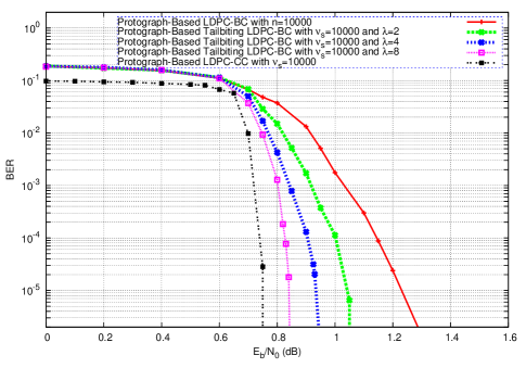
Figure 3: Simulation results for Example $3$.

We note that the protograph-based tail-biting LDPC convolutional codes outperform the underlying protograph-based LDPC block code (which can also be seen as a tail-biting code with unwrapping factor $\lambda=1$). Larger unwrapping factors yield improved error performance, eventually approaching the performance of the unterminated convolutional code, which can be seen as a tail-biting code with an infinitely large unwrapping factor. We also note that no error floor is observed for the convolutional code, which is expected, since the code ensemble is asymptotically good and has a relatively large ($\delta_{free}\geq 0.053$) distance growth rate.

We also note that the performance of the unterminated LDPC convolutional code is consistent with the iterative decoding threshold computed for the underlying protograph. At a moderate constraint length of $10000$, the unterminated code achieves $10^{-5}$ BER at roughly $0.12$ dB away from the threshold, and with larger block (constraint) lengths, the performance will improve even further. This is expected, since both the unterminated and the tail-biting convolutional codes preserve the same degree distribution as the underlying protograph.

VI Conclusions

In this paper, asymptotic methods were used to calculate a lower bound on the free distance that grows linearly with constraint length for several ensembles of unterminated, protograph-based periodically time varying LDPC convolutional codes. It was shown that the free distance growth rates of the LDPC convolutional code ensembles exceed the minimum distance growth rates of the corresponding LDPC block code ensembles. Further, we observed that the performance of the LDPC convolutional codes is consistent with the iterative decoding thresholds of the underlying protographs.

References

- [1] R. G. Gallager, “Low-density parity-check codes”, IRE Trans. Inform. Theory, IT-8: 21-28, Jan. 1962.
- [2] R. Michael Tanner, “A Recursive Approach to Low Complexity Codes”, IEEE Trans. Inform. Theory, IT-27, pp.533-547, Sept. 1981.
- [3] N. Wiberg, “Codes and decoding on general graphs”, Ph.D. Thesis, Dept. of E. E., Linköping University, Linköping, Sweden.
- [4] A. Jiménez-Felström and K. Sh. Zigangirov, “Time-varying periodic convolutional codes with low-density parity-check matrices”, IEEE Trans. Inform. Theory, IT-45, pp.2181-2191, Sept. 1999.
- [5] D. J. Costello, Jr., A. Pusane, S. Bates, and K. Sh. Zigangirov, “A comparison between LDPC block and convolutional codes”, Proc. Inform. Theory and App. Workshop, San Diego, CA, Feb. 2006.
- [6] D. J. Costello, Jr., A. E. Pusane, C. R. Jones, and D. Divsalar, “A comparison of ARA- and protograph-based LDPC block and convolutional codes”, Proc. Inform. Theory and App. Workshop, San Diego, CA, Feb. 2007.
- [7] M. Tavares, K. Sh. Zigangirov, and G. Fettweis, “Tail-Biting LDPC Convolutional Codes”, Proc. IEEE Int. Symp. on Inform. Theory, Nice, France, June 2007.
- [8] A. Sridharan, D. Truhachev, M. Lentmaier, D. J. Costello, Jr., and K. Sh. Zigangirov, “Distance bounds for an ensemble of LDPC convolutional codes”, IEEE Trans. Inform. Theory, IT-53, pp. 4537-4555, Dec. 2007.
-
[9]
D. Truhachev, K. Sh.
Zigangirov, and D. J. Costello, Jr., “Distance bounds for periodic