One-dimensional phase transitions in a two-dimensional optical lattice

Abstract

A phase transition for bosonic atoms in a two-dimensional anisotropic optical lattice is considered. If the tunnelling rates in two directions are different, the system can undergo a transition between a two-dimensional superfluid and a one-dimensional Mott insulating array of strongly coupled tubes. The connection to other lattice models is exploited in order to better understand the phase transition. Critical properties are obtained using quantum Monte Carlo calculations. These critical properties are related to correlation properties of the bosons and a criterion for commensurate filling is established.

1 Introduction

Atoms in optical lattices offer new versatile ways of studying many-body phenomena jessen1996 ; bloch2005 . Interference patterns of laser light provide periodic potentials for atoms, which are cooled to the nanokelvin range using laser and evaporative cooling. In this way, ground-state properties of these interesting many-body systems may be probed using a variety of optical techniques.

The optical potentials can be controlled with great range and precision, giving access to any kind of Bravais lattice as well as superlattices and quasiperiodic potentials grynberg2001 . The geometrical setup and choice of polarisation determine the lattice geometry, and the laser irradiance determines the amplitude of the potential. If the laser light is detuned to the red of the atomic transition, the potential will typically form an array of wells in which the atoms may be trapped if the potential is deep enough. The height and width of the potential barriers separating the wells determine the rate of tunnelling between them. In this way, the dimensionality of the sample can be controlled: making the potential barriers high enough in one Cartesian direction will effectively inhibit all tunnelling and result in a stack of independent, two-dimensional (2D) lattices. Increasing the potential along a second direction yields a 2D array of 1D tubes of atoms.

Recently, such dimensional crossovers in optical lattices and their relation to other theoretical models have attracted considerable attention. References ho2004 ; cazalilla2006 ; gangardt2006 studied a 2D array of one-dimensional tubes of atoms, known as Tomonaga-Luttinger liquids (TLL) giamarchi2004 . In a random-phase approximation, phase boundaries, coherence properties and excitation spectra were expressed in terms of the parameters that characterise the TLLs. In Ref. bergkvist2007 , we studied the corresponding situation in a 2D lattice geometry and investigated the relation between this model and a classical XY model sachdev1999 . It was determined that the transition between independent TLL tubes and a 2D superfluid is of Berezinskii-Kosterlitz-Thouless (BKT) type melko2004 ; weber1988 ; olsson1995b if the density is held fixed, and as an example, the critical point was determined for a specific value of tunnelling matrix element and filling.

In this paper, we further investigate the transitions in the 2D case. Using quantum Monte Carlo calculations, we investigate the link between coherence properties and the critical point for the phase transition. We confirm that the transition is determined by a TLL theory and that it depends crucially on the commensurability of the atoms in the lattice. In Sec. 2, we lay out the theory. In Sec. 3, we show how the present Hamiltonian is equivalent to other lattice models, which clarifies the nature of the phase transition. Section 4 explains the numerical method and the finite-size scaling performed in order to locate the phase transition, and presents the results for the phase transition at unit filling. In Sec. 5 we show how it is linked to the coherence properties. In Sec. 6, it is illustrated how changing one of the parameters of the theory allows for a crossing a two subsequent phase transitions. In Sec. 7, we investigate commensurability and density dependence, and finally in Sec. 8 we summarise and conclude.

2 Phase transitions in a 2D Hubbard model

Consider a one-component gas of bosonic atoms in a 3D lattice potential created by three standing waves at right angles,

$$V({\mathbf{r}})=V_{0x}\cos^{2}k_{\rm L}x+V_{0y}\cos^{2}k_{\rm L}y+V_{0z}\cos^{2}k_{\rm L}z,$$ (1)

where $k_{\rm L}=2\pi/\lambda$ is the angular wave number of the light, and the potential heights $V_{0x},V_{0y}$ and $V_{0z}$ are determined by the laser irradiance and detuning. In the tight-binding approximation, the many-body Hamiltonian is expanded in a basis of Wannier functions $w_{n}({\mathbf{r}}-{\mathbf{r}}_{i})$, each of which is localised in a well centred at position ${\mathbf{r}}_{i}$, where $i$ labels the wells and $n$ is a band index. If the wells are tight enough, and the atoms are cold enough, only the lowest-energy Wannier function within each well, $w_{0}({\mathbf{r}}-{\mathbf{r}}_{i})$, needs to be taken into account; this is the lowest Bloch band. The gas is then described by the bosonic single-band Hubbard model jaksch1998 ,

$$H=-\sum_{<ij>}t_{ij}(a_{i}a^{\dagger}_{j}+{\rm h.c.})+\frac{U}{2}\sum_{i}a^{\dagger}_{i}a^{\dagger}_{i}a_{i}a_{i}-\mu\sum_{i}a^{\dagger}_{i}a_{i},$$ (2)

where $i$ is a placeholder for the three indices $i_{x},i_{y},i_{z}$ enumerating the lattice sites in the Cartesian directions, and the sum subscripted $<\!\!ij\!\!>$ runs over pairs of neighbouring sites. The parameter $U$ is the on-site interaction strength, $t_{ij}$ is the tunnelling matrix element for the barriers between sites $i$ and $j$, and $\mu$ is the chemical potential, adjusted in the calculations to give the desired density of atoms. The on-site interaction strength is defined as

$$U=\frac{2\pi\hbar^{2}a}{m}\int\mathrm{d}^{3}r|w_{0}({\mathbf{r}}-{\mathbf{r}}_{i})|^{4},$$ (3)

where $a$ is the s-wave scattering length of the atoms and $m$ is the atomic mass. Since this optical lattice is created by three independent pairs of standing waves, the tunnelling matrix element $t_{ij}$ in one particular term takes on one of three values. If the wells $i$ and $j$ are neighbours along the $x$ direction, its value is

$$t_{x}=\int\mathrm{d}^{3}{\mathbf{r}}w_{0}^{*}(x,y,z)\left[-\frac{\hbar^{2}}{2m}\nabla^{2}+V({\mathbf{r}})\right]w_{0}(x+d,y,z),$$ (4)

where $d=\lambda/2$ is the lattice spacing. The tunnelling matrix elements $t_{y}$ and $t_{z}$ are defined similarly.

It turns out that the tunnelling matrix elements depend exponentially on the potential depth jaksch1998 . As a result, one can easily make $t_{x}$, $t_{y}$ and $t_{z}$ differ by orders of magnitude by a judicious choice of the laser irradiances. Thus, $V_{0z}$ can be chosen large enough that $t_{z}$ can be neglected and the sample is effectively 2D. In the following, we confine the discussion to the 2D Bose-Hubbard model (henceforth referred to as the Hubbard model for brevity). The phase diagram is sketched in Fig. 1 and we now describe the general features.

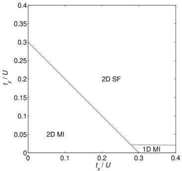
Figure 1: Predicted phases of the anisotropic Hubbard model in two dimensions. “2D MI” and “2D SF” stand for the two-dimensional Mott insulating phase and superfluid phase, respectively. The phase “1D MI” is predicted to exist only when one of the side lengths of the system is finite. In this figure, the system extends infinitely along the $y$ direction and is 4 sites wide in the $x$ direction. The slight decrease of the corresponding phase boundary is not visible in the figure.

When both $t_{x}$ and $t_{y}$ are small compared with $U$, and in addition the number of bosons is commensurate with the number of lattice sites, the sample is Mott insulating (MI), with exponentially decaying phase correlations and suppressed fluctuations in the number of particles per site. In the opposite limit, when $t_{x}$ and $t_{y}$ are of the same order as $U$ or larger, the ground state is the 2D superfluid (2D SF) state, characterised by long-range phase coherence in 2D and a fluctuating number of particles per site. In one dimension with one particle per site, there is a quantum phase transition between these phases at $t/U=0.3$ kuhner2000 . In higher dimensions, one may apply a mean-field approximation sachdev1999 , dictating that the transition occurs when the sum of all matrix elements equals the 1D value, i.e.,

$$\frac{t_{x}+t_{y}}{U}=0.3$$ (5)

in two dimensions. The exact, numerically obtained 2D result freericks1996 deviates slightly from this mean-field result. Furthermore, quantum Monte Carlo calculations performed on finite systems tend to underestimate the critical value for the phase transition.

If one of the tunnelling matrix elements, say $t_{x}$, is relatively large and the other, $t_{y}$, is small, there may in fact under certain circumstances exist a phase where there is superflow along one dimension but not along the other. Such a state will be called the 1D MI phase. It turns out that in an infinite 2D system, such a state is absent: if there is superflow in the $x$ direction, then any nonzero tunnelling along the $y$ direction will put the sample into the 2D SF state efetov1974 (as a corollary, any finite tunnelling along the $z$ direction will result in a 3D SF state). However, as was first noted by Ho et al. and Gangardt et al. ho2004 ; cazalilla2006 ; gangardt2006 (although applied to the 3D case), the situation changes when the sample is finite along the strongly coupled $x$ direction. The system can then be thought of as an array of finite tubes lining up along the $y$ direction and extending along the $x$ direction.

Because of the finite excitation energy within the tubes, there can now exist a 1D MI phase if $t_{y}$ is sufficiently small. By the same argument, the tunnelling along the $z$ direction can be neglected, as we assumed.

In a finite system, there is no true phase transition. In practice, this is not a problem since the phase transition is replaced by a crossover. In theory, it is always possible to let the system extend indefinitely along the weakly coupled $y$ direction, while keeping it finite along the $x$ direction. There is then a true phase transition between insulating and superfluid behaviour along the $y$ direction. We call this the 1D MI - 2D SF transition.

In Refs. ho2004 ; cazalilla2006 ; gangardt2006 , the 1D tubes were described using TLL theory. This theory describes a 1D many-body system, which is characterised by two parameters independently of statistics and the detailed properties of the constituent particles, namely the sound velocity $v_{\rm s}$ and the TLL parameter $K$, defined as

$$K=\frac{v_{\rm F}}{v_{\rm s}}.$$ (6)

Here, $v_{\rm F}=\hbar\pi\rho/(md)$, where $\rho$ is the filling factor, i.e., the number of bosons per site, and $d$ is the lattice constant. The TLL parameter $K$ determines the behaviour of the particle-particle correlations $\Gamma(i,j)$, which obey the power law

$$\Gamma(i,j)\equiv\langle a^{\dagger}_{i}a_{j}\rangle\propto|{\mathbf{r}}_{i}-{\mathbf{r}}_{j}|^{-1/(2K)}.$$ (7)

For the discussion of the correlations along different directions, we introduce the notation $\Gamma_{x}$ and $K_{x}$ for the correlations within the strongly coupled tubes, as well as $\Gamma_{y}$ and $K_{y}$ for describing correlations along the weakly coupled $y$ direction.

Since a larger $K_{x}$ implies greater coherence along the $x$ direction, we expect $K_{x}$ to increase with $t_{x}/U$. Furthermore, it is a known exact result that

$$2\leq K_{x}<\infty$$ (8)

for a system of lattice bosons with only on-site interactions giamarchi2004 . If one further decreases the tunnelling beyond the point where $K_{x}=2$, one enters the MI phase. However, the quantitative relation between $t_{x}$ and $K_{x}$ is not known in closed form.

3 Equivalence to other lattice models

In order to obtain an expression for the transition point, the TLL tubes were in Refs. ho2004 ; cazalilla2006 treated as structureless sites by integrating out all degrees of freedom except a number operator $N_{j}$ and a phase operator $\phi_{j}$ for each tube (the analysis was done with a 3D system in mind, but the results apply to the 2D case as well). In that way, a number-phase model vanotterlo1995 was obtained with a governing Hamiltonian

$$H=-E_{\rm J}\sum_{<ij>}\cos(\phi_{i}-\phi_{j})+E_{\rm C}\sum_{i}(N_{i}-N_{0})^{2},$$ (9)

where $N_{0}$ is the equilibrium number of particles per tube, and $<\!\!ij\!\!>$ denotes neighbouring tubes in the $y$ direction. $E_{\rm J}$ is usually referred to as the tunnelling energy and $E_{\rm C}$ as the charging energy. The mapping is expected to hold in the 1D MI phase, but above the phase transition, where the whole 2D system is superfluid, it may not be valid. It was found in Refs. ho2004 ; cazalilla2006 that

$$E_{\rm J}=t_{y}N_{0}^{1-\alpha_{x}},$$ (10)

and

$$E_{\rm C}=\frac{C_{0}U}{L_{x}},$$ (11)

where the exponent

$$\alpha_{x}=\frac{1}{2K_{x}}.$$ (12)

Thus, it is predicted that the behaviour of the particle-particle correlation function within the tubes determines the location of the critical point for the decoupling of the tubes. Here, $L_{x}$ is the number of sites that the lattice extends in the $x$ direction, and $C_{0}$ is a constant that can in general not be obtained in closed form. The number-phase Hamiltonian undergoes a SF-MI quantum phase transition at the critical point where

$$\frac{E_{\rm J}}{E_{\rm C}}={\rm constant},$$ (13)

where the right-hand side is a universal numerical constant to be determined. Hence, for the critical value $t_{y\rm c}$ of $t_{y}$,

$$\frac{t_{y\rm c}}{U}\propto\rho^{-1+\alpha_{x}}L_{x}^{-2+\alpha_{x}},$$ (14)

as long as the analysis of Ref. ho2004 ; cazalilla2006 provides a valid model for the anisotropic optical lattice. The same functional form for the critical point was obtained in Ref. gangardt2006 by means of a random-phase approximation. In Eq. (14), the filling $\rho$ is defined as the mean number of atoms per lattice site, and is thus dimensionless. Due to the known constraints on $K_{x}$, the power on $L_{x}$ lies between -1.75 and -2, where the former holds close to the transition to a 2D MI. We define the effective coupling constant

$$\tilde{t}_{y}=\frac{t_{y}}{U}L_{x}^{2-\alpha_{x}}\rho^{1-\alpha_{x}}.$$ (15)

Stated in terms of this quantity, the critical value of the tunnelling $t_{y}$ can be written as

$$\frac{t_{y\rm c}}{U}=\tilde{t}_{y\rm c}L_{x}^{-2+\alpha_{x}}\rho^{-1+\alpha_{x}},$$ (16)

where $\alpha_{x}$ and $\tilde{t}_{y\rm c}$ are constants to be determined.

The nature of the quantum phase transition in the number-phase model can be understood by making use of the general result that a quantum phase transition in $D$ dimensions is in the same universality class – i.e., it has the same critical properties – as a classical phase transition in a certain corresponding model in $D+1$ dimensions sachdev1999 . In 1D, with the number of bosons kept fixed, the transition studied here is in the same universality class as the classical XY model in 2 dimensions at a finite temperature $T_{\rm XY}=1/(k_{\rm B}\beta_{\rm XY})$. The mapping is accomplished by identifying sondhi1997

$$\beta_{\rm XY} = \sqrt{\frac{E_{\rm J}}{E_{\rm C}}},$$

$$L_{x,\rm XY} = \beta\sqrt{E_{\rm J}E_{\rm C}},$$

$$L_{y,\rm XY} = L_{y},$$ (17)

where quantities with the subscript XY refer to the 2D XY model and quantities without that subscript refer to the number-phase model. In terms of the underlying anisotropic Hubbard model, we can thus write

$$\beta_{\rm XY} = \left(\frac{t_{y}L_{x}^{2-\alpha_{x}}\rho^{1-\alpha_{x}}}{C_{0}U}\right)^{1/2},$$

$$L_{x,\rm XY} = \beta\left(C_{0}Ut_{y}L_{x}^{-\alpha_{x}}\rho^{1-\alpha_{x}}\right)^{1/2},$$

$$L_{y,\rm XY} = L_{y},$$ (18)

where $C_{0}$ is the same constant as in Eq. (11), and $\beta=1/(k_{\rm B}T)$, where $T$ is the temperature of the Hubbard model. This mapping shows that if the XY model has a phase transition at an inverse temperature $\beta_{\rm XY}$, then the Hubbard model has a quantum phase transition when $\tilde{t}_{y}$ reaches a critical value, consistent with Eq. (16). The critical point will depend on the tunnelling within the tubes, $t_{x}$, through the Luttinger parameter $K_{x}$ and also through the unknown constant of proportionality $C_{0}$ in Eq. (18).

The 2D XY model exhibits a BKT transition melko2004 ; fisher1989 ; krauth1991 ; kuhner1998 . This kind of transition possesses several characteristics, among them a universal jump in the superfluid density at the transition point. According to the series of mappings performed here, from a 2D anisotropic Hubbard model via a 1D number-phase model to a 2D XY model, the anisotropic Hubbard model exhibits a BKT transition. The findings of Ref. bergkvist2007 confirm these expectations, and the present paper further expands on the subject.

4 Finite size scaling

In the numerical calculations, the 2D Hubbard model was simulated using the stochastic series expansion method syljuasen2002 ; syljuasen2003 . The chemical potential $\mu$ was tuned to obtain the desired mean number of particles. By selecting those Monte Carlo steps that correspond to a fixed number of particles, it was made sure that the calculations were performed at a given density, which is important for the characteristics of the phase transition. We chose $\beta=1000U^{-1}$ in order to make sure that ground-state properties were calculated, and the number of states per site was chosen to 6 in order to ensure convergence.

Systems of $L_{x}\times L_{y}$ sites were simulated, where the side lengths $L_{x}$ and $L_{y}$ were varied in order to assess the predicted dependence of the critical point on the length discussed in Sec. 2. The boundary conditions were chosen to be periodic, which is necessary for calculating the superfluid density as will be described. The most important calculated quantities are the superfluid density $\rho_{\rm s}$ and the particle-particle correlations $\Gamma_{x}$ and $\Gamma_{y}$. The superfluid density is numerically computed via the winding number $W_{y}$ as

$$\rho_{\rm s}=\frac{\langle W_{y}^{2}\rangle L_{y}}{L_{x}\beta},$$ (19)

where $W_{y}$ is the net number of times that a particle line crosses the periodic boundary in the $y$ direction in the simulations melko2004 . The superfluid density as a function of the ratio of tunnelling matrix element and on-site interaction energy, $t_{y}/U$, is plotted in Fig. 2 for a few examples of parameter values.

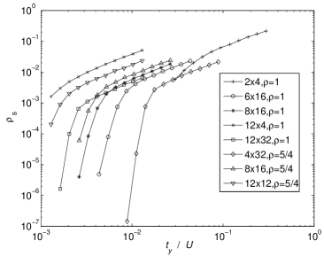
Figure 2: A few arbitrarily selected curves showing the superfluid density as a function of the ratio of tunnelling $t_{y}$ to on-site interaction $U$. The different curves correspond to different data sets obtained at different fixed side lengths $L_{x}$ and $L_{y}$, and different filling factors $\rho$.

It is clear that the curves make a sharp drop at a transition point when $t_{y}/U$ becomes small enough. The transition point seems to depend on both $L_{x}$ and $\rho$, as was predicted in Sec. 3, and we now turn to the problem of calculating this dependence.

In order to locate the critical point, finite-size scaling must be performed weber1988 ; olsson1995b ; melko2004 . However, the analysis of the present problem presents several difficulties compared with a classical XY model. At the BKT transition, the superfluid density assumes a value known as the universal jump, proportional to the critical temperature. This is routinely used in 2D XY-model simulations, but since in the present case the two quantities are only known to within an unknown constant, we cannot make use of this relation. Moreover, the mapping between the Hubbard model and the 2D XY model is only valid at and below the phase transition. In the 2D SF phase, the coherence between tubes may be comparable to that within the tubes and the mapping is not valid. Finally, a quantum Monte Carlo calculation of the 2D Hubbard model is very time consuming and in the parameter regime of interest, where the parameters $t_{x}$ and $t_{y}$ differ by orders of magnitude, it is hard to obtain data with high accuracy. This is aggravated by the fact that the side length $L_{y}$ varies between 4 and 32 in the simulations.

As seen in Sec. 3, the anisotropic Hubbard model is predicted to have the same properties close to the transition as the 2D XY model has close to the BKT transition, if the 2D XY model has a superfluid density given by

$$\rho_{\rm s,XY}=\frac{\langle W_{y}^{2}\rangle L_{y}}{\beta t_{y}\rho^{1-\alpha_{x}}L_{x}^{1-\alpha_{x}}}.$$ (20)

The BKT transition occurs when $\tilde{t}_{y}$ assumes a critical value; at this point, all the curves $\rho_{\rm s,XY}(\tilde{t}_{y};L_{x};L_{y})$ computed for different parameter values should ideally coincide (taking finite-size effects into account). This means that $\alpha_{x}$ has to be optimised so that all the curves for different parameter values coincide as closely as possible. This is accomplished by first considering sets of data series with a given $L_{y}$ and different $L_{x}$. If the analysis in Sec. 3 is correct, then all systems of size $L_{x}\times L_{y}$ can be approximated as 1D chains of length $L_{y}$, and therefore the results for $\rho_{\rm s,XY}$ as a function of $\tilde{t}_{y}$ should coincide between data series with similar $L_{y}$ and different $L_{x}$, if only the parameter $\alpha_{x}$ is chosen correctly. As noted in Sec. 3, the correspondence is only expected to hold in the 1D MI phase, so that for $\tilde{t}_{y}>\tilde{t}_{y\rm c}$, one cannot require the data to coincide. Thus, one needs to consider the variance among the curves below a supposed critical point, and choose the value of $\alpha_{x}$ that minimises the variance. This is to be done for each $L_{y}$ separately, and then the results for different $L_{y}$ can be compared. We thus do a spline interpolation of the points over the relevant range of $\tilde{t}_{y}$ and compute, for a given $L_{y}$ and $\alpha_{x}$,

$${\rm Var}(\rho_{\rm s,XY})(\tilde{t}_{y},\alpha_{x},L_{y})=$$

$$\sum_{L_{x}}\left(\rho_{\rm s,XY}(\tilde{t}_{y};L_{x};L_{y})-\frac{1}{N_{L_{x}}}\sum_{L_{x}}\rho_{\rm s,XY}(\tilde{t}_{y};L_{x};L_{y})\right)^{2},$$ (21)

and furthermore the summed variance over the whole range of $\tilde{t}_{y}$ is

$$\overline{\rm Var}(\rho_{\rm s,XY})(\alpha_{x},L_{y})=\frac{\int\mathrm{d}\tilde{t}_{y}{\rm Var}(\rho_{\rm s,XY})(\tilde{t}_{y},\alpha_{x},L_{y})}{\int\mathrm{d}\tilde{t}_{y}1}.$$ (22)

In Eqs. (21-22), $N_{L_{x}}$ is defined as the number of different values of $L_{x}$ used. Since the curves are supposed to coincide only below the critical point, the integration limits for $\tilde{t}_{y}$ are chosen as $0\leq\tilde{t}_{y}\leq 0.3$, anticipating the result that the critical point is close to $\tilde{t}_{y\rm c}=0.3$. The result does not depend strongly on the chosen integration limits.

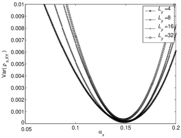
Figure 3: Variance in the superfluid density among data sets as a function of the unknown exponent $\alpha_{x}=1/(2K_{x})$.

For each value of $L_{y}$, we obtain an optimal value for $\alpha_{x}$. Averaging over different $L_{y}$, the result is

$$\alpha_{x}=0.15,$$ (23)

resulting in

$$K_{x}=3.4.$$ (24)

When data for different system sizes $L_{y}$ are compared, they are expected to coincide at the critical point, but not below or above. In addition, the coincidence of the curves is exact only in the limit $L_{y}\to\infty$, but it is known how to make the lowest-order correction for finite $L_{y}$. At the BKT transition point in the 2D XY model, the superfluid density depends asymptotically on the size of the finite sample as

$$\rho_{\rm s,XY}(\infty)=\frac{\rho_{\rm s,XY}(L_{y})}{1+\frac{1}{2\ln(L_{y})+C}},$$ (25)

where $\rho_{\rm s,XY}(L_{y})$ is the superfluid density computed using a side length $L_{y}$. This result is known as Weber-Minnhagen scaling weber1988 , and in Ref. melko2004 it was found that the procedure applies to non-quadratic systems as long as the winding number is computed along the shorter dimension of the sample. In our effective XY model, $L_{x,\rm XY}$ is proportional to the inverse temperature of the Hubbard model and it is thus much larger than $L_{y}$. The constant $C$ was in Ref. olsson1995b found to be equal to 1.8.

Figure 4 collects the simulated data for all different values of $L_{x}$ and $L_{y}$. Ideally, all the data is expected to coincide at the critical point $\tilde{t}_{y\rm c}$.

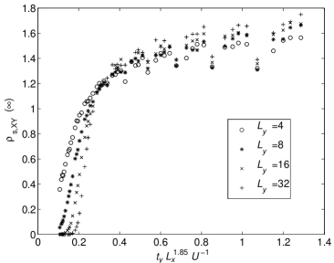
Figure 4: Superfluid density for the dual XY model, scaled using the best fit parameter $K_{x}=3.4$, for a filling $\rho=1$. The plot contains all the data sets used in the scaling. The values of $L_{y}$ are as indicated in the legend.

The variance among these curves is now recorded as a function of $\tilde{t}_{y}$ and the smallest variance is at

$$\tilde{t}_{y\rm c}=0.33.$$ (26)

Table 1 summarises the computed parameters for a few different values of tunnelling $t_{x}$ and filling $\rho$. The constant $\tilde{t}_{y\rm c}$ was defined in Eq. (16), the exponent $\alpha_{x}$ and the result for $K_{x}$ are as obtained above, and the value for $K_{x}$ obtained from correlations will be discussed in Sec. 5.

Table 1: Parameters determining the 2D SF-1D MI transition. The method to calculate the error bars are described in the text. The data for $t_{x}/U=0.3$ are lifted from Ref. bergkvist2007 .

$t_{x}/U$	$\rho$	$\tilde{t}_{y\rm c}$	$\alpha_{x}$	$K_{x}$	$K_{x}$
				(transition)	(correlation)
0.3	1.0	0.3	0.25	2.0	–
0.5	1.0	0.33	0.15	3.4	3.0
0.5	5/4	0.32	0.15	3.4	2.7
0.5	19/16	-	-	-	2.1

In order to check the above results, we apply a different scaling procedure, by bunching together results for the same $L_{x}$ but different $L_{y}$. If the superfluid density, corrected as in Eq. (25), is computed for a range of $L_{y}$ values and a fixed $L_{x}$, the dependence on $L_{x}$ cancels out and the curves should coincide at the critical point. The dependence of the critical point on $L_{x}$ can then be calculated. Figure 5 shows how this method works.

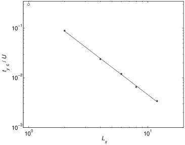
Figure 5: Upper: An example of data collapse for the superfluid density scaled according to Weber-Minnhagen scaling, at side length $L_{x}=8$. Lower: Measured critical tunnelling as a function of side length $L_{x}$; the dependence is expected to be a power law. The linear fit yields $\alpha_{x}=0.17$, giving $K_{x}=2.9$. The circle indicates the previously obtained critical point for the Mott transition in the 1D Hubbard model, $L_{x}=1$.

The point $t_{y\rm c}/U$, at which the variance of the Weber-Minnhagen scaled superfluid density across different $L_{y}$ is a minimum, is recorded for each fixed value of $L_{x}$. (The result for $L_{x}=8$ is indicated with an arrow in the upper panel of Fig. 5.) Then $t_{y\rm c}/U$ as a function of $L_{x}$ is fitted to a power-law dependence, as illustrated in the lower panel of Fig. 5. The best linear fit to the log-log-curve is given by $t_{c}=0.31L_{x}^{-1.83}$. In the figure, we have also inserted the previously obtained result $\tilde{t}_{y\rm c}=0.30$ for the case $L_{x}=1$, which is just the 1D Hubbard model kuhner2000 . Fig. 5 is a qualitative support for the prediction of Refs. ho2004 ; cazalilla2006 ; gangardt2006 that the critical coupling decreases as a power-law function of $L_{x}$, with a power slightly below 2.

5 Phase transition and correlations

One important prediction made in Refs. ho2004 ; cazalilla2006 ; gangardt2006 is that the dependence on the transition point $t_{y\rm c}$ on tube length $L_{x}$ is linked to the behaviour of the particle-particle correlations in an isolated tube. In order to test this, we compute the correlation function $\Gamma_{x}(i_{x})$, where $i_{x}$ is the number of lattice sites separating two points in the $x$ direction. An example of a computed correlation function is shown in Fig. 6.

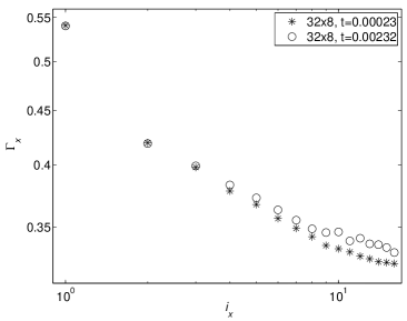
Figure 6: Particle-particle correlation function in the $x$ direction. The correlation function $\Gamma_{x}$ is shown as a function of coordinate $i_{x}$ for filling $\rho=1$, $t_{x}/U=0.5$, $L_{x}=32$, $L_{y}=8$, $t_{y}/U=2.32\times 10^{-4}$ ($\ast$), and $t_{y}/U=2.32\times 10^{-3}$ ($\circ$).

The correlation function is fitted to a power law according to Eq. (7). It is seen in Fig. 6 that the correlations in the strongly coupled $x$ direction depend on the tunnelling in the weakly coupled $y$ direction (just as the opposite relation holds). Since the predictions of Refs. ho2004 ; cazalilla2006 ; gangardt2006 build on the correlation properties of an isolated tube, we should use the results obtained for the smallest values of $t_{y}$, in the 1D MI phase, where the tubes are decoupled. We find the value $K_{x}=3.0$ for $t_{x}=0.5U$ and filling $\rho=1$. This is consistent with the value $K_{x}=3.4$ found from finite-size scaling in Sec. 4.

6 Dependence on in-tube tunneling

As a way to visualise the three predicted phases, we show as an example in Fig. 7 the result of a calculation where the tunnelling in the strongly coupled $x$ direction, $t_{x}$, has been changed while $t_{y}$ is kept constant at $t_{y}=0.003U$.

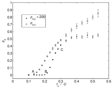
Figure 7: Superfluid density in the $x$ and $y$ directions, respectively, for a Bose-Hubbard model of size 12$\times$12 lattice sites, fixed tunnelling $t_{y}/U=0.003$, and a filling of one atom per site. The scale for $\rho_{s,y}$ has been expanded by a factor 200. The points labelled A, B, and C are discussed in the text.

This corresponds to moving along a horizontal line in the lower part of the phase diagram in Fig. 1. (Observe, however, that Fig. 1 corresponds to the case $L_{x}=4$, while here $L_{x}=12$, and therefore the position of the phase boundary is shifted.) The parameters are chosen such that, anticipating the results in Sec. 4, the system should pass from the 2D MI phase, via the 1D MI phase, into the 2D SF phase. The calculation is done for a finite lattice with 12$\times$12 sites, and the superfluid densities corresponding to motion in the $x$ and $y$ directions, respectively, are found. It is seen that the superfluid density corresponding to the $x$ direction begins to increase first, at the point labelled A, and the increase of $\rho_{s,y}$ commences at the later point B. This is precisely what is expected for a system that crosses the two transition lines. However, one should note that the increase of $\rho_{s,y}$ seems to saturate at point C, and at the same point, the slope of the curve for $\rho_{s,x}$ is also seen to slightly decrease.

In fact, when one tunes $t_{x}$ such that the 2D MI, 1D MI, and 2D SF phases are visited in turn, then both phase transitions belong to the BKT universality class. Furthermore, experience shows that it is the onset of the drop from a finite value, not the onset of a rise from a value close to zero, that should be identified with the BKT transition point. In Fig. 7 it thus seems that it is the point labelled C, rather than the points labelled A and B, that indicates the true transition, and one can conclude that the transitions associated with the strong and weak couplings occur (within calculated error bars) at the same point. This is also what the theory for the infinite system dictates: there is no 1D MI phase if both $L_{x}$ and $L_{y}$ are taken to infinity. Here, however, we are concerned with finite systems, so we should not take the limit of infinite $L_{x}$. The figure shows clearly that in the finite system, there is a region in which the superflow along the $x$ direction is non-negligible but that along the $y$ direction is very small. This is the 1D MI phase, but it cannot be found by applying finite-size scaling for the $x$ direction.

7 Phase transition at non-integer density

We return to Eq. (16), obtained from Refs. ho2004 ; cazalilla2006 ; gangardt2006 , which predicts that the transition point $t_{y\rm c}/U$ has a power-law dependence on both the length $L_{x}$ and filling $\rho$ of the tubes. However, the 1D MI phase only exists if there is an integer number of bosons in each tube, i.e., if the filling is commensurate with respect to the number of tubes. The number of particles per site, on the other hand, does not have to be an integer. To check this, and thus establish that we are indeed seeing a Mott transition along one direction, we study the cases $\rho=5/4$ and $\rho=19/16$, respectively. In the first case, the tube length, $L_{x}$, is chosen as a multiple of 4 in order to ensure commensurability, and in the second case, we choose values of $L_{x}$ that are not divisible by 16, in order to avoid commensurability. The results are shown in Fig. 8.

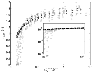
Figure 8: Superfluid density in the XY model, $\rho_{\rm s,XY}$, for a number of data sets. Data is taken at the commensurate density $\rho=1$ ($\circ$); commensurate tube filling with $\rho=5/4$ ($\bigtriangledown$); and the incommensurate filling $\rho=19/16$ ($\ast$). Here, $t_{x}/U=0.5$, the value of $L_{x}$ for the different curves varies between 2 and 32, and $L_{y}$ between 4 and 32. The quantities on the axes are the best fits to finite-size scaling for the coupling and superfluid density, respectively. The inset shows the same data in a log-log plot.

The finite-size scaling was performed as described in Sec. 4. In the commensurate case, $\rho=5/4$, a phase transition is found. For the incommensurate case, $\rho=19/16$, the data may be collapsed with the best-fit result $K_{x}=3.6$, and $\tilde{t}_{y\rm c}=0.21$. However, it is seen in Fig. 8 that the superfluid density for this incommensurate density does not go steeply to zero when $t_{y}$ is decreased below the calculated critical point, even for the largest system size $L_{y}=32$. Instead, the data is clearly consistent with the curves meeting the $x$ axis at the origin, unlike the commensurate cases $\rho=1$ and $\rho=5/4$. We conclude that the data corroborates the conclusion that the filling per tube needs to be integer in order for the 1D MI phase to exist.

8 Conclusions

In this paper, we have studied bosons trapped in two-dimensional optical lattices by Monte-Carlo calculations, with the objective of characterising phase transitions and their dependence on dimensionality and lack of isotropy. Apart from the expected phases, where one have superfluidity or Mott insulation along both directions, we show that there also can exist situations where atoms may tunnel along one direction, while not along the other. This means having superfluidity, and accordingly strong correlations, in only one of the two available dimensions. We call this phase a one-dimensional Mott insulator.

We study the transition to this phase from a two-dimensional superfluid and explore the conditions for this phase transition to occur. We find that the transition point depends on a specific combination of the weaker tunnelling matrix element $t_{y}$, the on-site interaction strength $U$, the number of sites in the strongly coupled direction $L_{x}$, the filling $\rho$, and in addition the Luttinger parameter $K_{x}$, which depends on the stronger tunnelling matrix element $t_{x}$. The transition point and the Luttinger parameter are both calculated.

We also verify that the location of the phase transition is connected to the decay of particle-particle correlations in a manner consistent with predictions based on Tomonaga-Luttinger liquid theory ho2004 ; cazalilla2006 ; gangardt2006 , and that the transition occurs when the number of particles is commensurate with the side length of the system in the direction of weak tunnelling, but not necessarily with the number of sites.

- (1) P. Jessen and I. Deutsch, Adv. Atom. Mol. Opt. Phys. 37, 95 (1996).
- (2) I. Bloch, Nature Physics 1, 23 (2005).
- (3) G. Grynberg and C. Robilliard, Phys. Rep. 355, 335 (2001).
- (4) A. F. Ho, M. A. Cazalilla, and T. Giamarchi, Phys. Rev. Lett. 92, 130405 (2004).
- (5) M. A. Cazalilla, A. F. Ho, and T. Giamarchi, New J. Phys 8, 158 (2006).
- (6) D. Gangardt, P. Pedri, L. Santos, and G. Shlyapnikov, Phys. Rev. Lett. 96, 040403 (2006).
- (7) T. Giamarchi, Quantum Physics in One Dimension (Clarendon, Oxford, 2004).
- (8) S. Bergkvist et al., Phys. Rev. Lett. 99, 110401 (2007).
- (9) S. Sachdev, Quantum Phase Transitions (Cambridge University Press, Cambridge, 1999).
- (10) R. G. Melko, A. W. Sandvik, and D. J. Scalapino, Phys. Rev. B 69, 014509 (2004).
- (11) H. Weber and P. Minnhagen, Phys. Rev. B 37, 5986 (1988).
- (12) P. Olsson, Phys. Rev. B 52, 4526 (1995).
- (13) D. Jaksch et al., Phys. Rev. Lett. 81, 3108 (1998).
- (14) T. D. Kühner, S. R. White, and H. Monien, Phys. Rev. B 61, 12474 (2000).
- (15) J. K. Freericks and H. Monien, Phys. Rev. B 53, 2691 (1996).
- (16) K. B. Efetov and A. I. Larkin, Sov. Phys.–JETP 39, 1129 (1974).
- (17) A. van Otterlo et al., Phys. Rev. B 52, 16176 (1995).
- (18) S. L. Sondhi, S. M. Girvin, J. P. Carini, and D. Shahar, Rev. Mod. Phys. 69, 315 (1997).
- (19) M. P. A. Fisher, P. B. Weichman, G. Grinstein, and D. S. Fisher, Phys. Rev. B 40, 546 (1989).
- (20) W. Krauth and N. Trivedi, Europhys. Lett. 14, 627 (1991).
- (21) T. D. Kühner and H. Monien, Phys. Rev. B 58, R14741 (1998).
- (22) O. Syljuåsen and A. W. Sandvik, Phys. Rev. E 66, 046701 (2002).
- (23) O. Syljuåsen, Phys. Rev. E 67, 046701 (2003).