Bayesian strong gravitational-lens modelling on adaptive grids:
objective detection of mass substructure in galaxies

Abstract

We introduce a new adaptive and fully Bayesian grid-based method to model strong gravitational lenses with extended images. The primary goal of this method is to quantify the level of luminous and dark-mass substructure in massive galaxies, through their effect on highly-magnified arcs and Einstein rings. The method is adaptive on the source plane, where a Delaunay tessellation is defined according to the lens mapping of a regular grid onto the source plane. The Bayesian penalty function allows us to recover the best non-linear potential-model parameters and/or a grid-based potential correction and to objectively quantify the level of regularization for both the source and the potential. In addition, we implement a Nested-Sampling technique to quantify the errors on all non-linear mass model parameters – marginalized over all source and regularization parameters – and allow an objective ranking of different potential models in terms of the marginalized evidence. In particular, we are interested in comparing very smooth lens mass models with ones that contain mass-substructures. The algorithm has been tested on a range of simulated data sets, created from a model of a realistic lens system. One of the lens systems is characterized by a smooth potential with a power-law density profile, twelve include a Navarro, Frenk and White (NFW) dark-matter substructure of different masses and at different positions and one contains two NFW dark substructures with the same mass but with different positions. Reconstruction of the source and of the lens potential for all of these systems shows the method is able, in a realistic scenario, to identify perturbations with masses $\ga 10^{7}\rm M_{\odot}$ when located on the Einstein ring. For positions both inside and outside of the ring, masses of at least $10^{9}\rm M_{\odot}$ are required (i.e. roughly the Einstein ring of the perturber needs to overlap with that of the main lens). Our method provides a fully novel and objective test of mass substructure in massive galaxies.

1 Introduction

At the present time, the most popular cosmological model for structure formation is the $\Lambda\text{CDM}$ paradigm. While this model has been very successful in describing the Universe on large scales and in reproducing numerous observational results (e.g., Reiss et al. 1998; Efstathiou et al. 2002; Burles et al. 2001; Phillips et al. 2001; Jaffe et al. 2001; Percival et al. 2001; de Bernardis et al. 2002; Hamilton & Tegmark 2002; Croft et al. 2002; Tonry et al. 2003; Spergel et al. 2003; Komatsu et al. 2008), important discrepancies still persist on small scales. In particular, some of these involve the dark matter distribution within galactic haloes (e.g., Moore 1994; Burkert 1995; McGaugh & de Blok 1998; Binney & Evans 2001; de Blok et al. 2001; de Blok & Bosma 2002; McGaugh et al. 2003; Simon et al. 2003; Rhee et al. 2004; Kuzio de Naray et al. 2006) and the number of galaxy satellites, i.e the Missing Satellite Problem.

According to the standard scenario, structures form in a hierarchical fashion via merging and accretion of smaller objects (Toomre 1977; Frenk et al. 1988; White & Frenk 1991; Barnes 1992; Cole et al. 2000). As shown by the latest numerical simulations, in which high mass and force resolution is achieved, the progenitor population is only weakly affected by virialization processes and a large number of sub-haloes is able to survive after merging. The number of substructures within the Local Group, however, is predicted to be 1-2 orders of magnitude higher than what is effectively observed (e.g., Kauffmann et al. 1993; Moore et al. 1999; Klypin et al. 1999; Moore et al. 2001; Diemand et al. 2007a, b).

Two different classes of solutions have been suggested to alleviate this problem, cosmological and astrophysical. Cosmological solutions address the basis of the $\Lambda\text{CDM}$ paradigm itself and mostly concentrate on the properties of the dark matter, allowing for example, for a warm (Colin et al. 2000), decaying (Cen 2001), self-interacting (Spergel & Steinhardt 2000), repulsive (Goodman 2000), or annihilating nature (Riotto & Tkachev 2000). Alternatively the $\Lambda\text{CDM}$ picture can be modified by the introduction of a break of the power-spectrum at the small scales (e.g., Kamionkowski & Liddle 2000; Zentner & Bullock 2003).

From an astrophysical point of view, the number of visible satellites can be reduced by suppressing the gas collapse/cooling (e.g., Bullock et al. 2000; Kravtsov et al. 2004; Moore et al. 2006) via supernova feedback, photoionization or reionization. This would result in a high mass-to-light ratio ($M/L$) in the substructures. If these high-$M/L$ substructures indeed exist, different methods for indirect detection are possible. The dark substructure may be detectable for example through its effects on stellar streams (e.g., Ibata et al. 2002; Mayer et al. 2002), via $\gamma$-rays from dark matter annihilation (Bergström et al. 1999; Calcáneo-Roldán & Moore 2000; Stoehr et al. 2003; Colafrancesco et al. 2006) or through gravitational lensing (e.g., Dalal & Kochanek 2002; Koopmans 2005).

While the first two approaches are limited to the local Universe, gravitational lensing allows one to explore the mass distribution of galaxies outside the Local Group and at a relatively high redshift. Moreover, gravitational lensing is independent of the baryonic content, of the dynamical state of the system and of the nature of dark matter. For example, when in a lens system a point source is close to the caustic fold or cusp, the sum of the image fluxes should add to zero if the sign of the image parities is taken into account (Blandford & Narayan 1986; Zakharov 1995). This relation is, however, violated by many observed lensed quasars with cusp and fold images. As first suggested by Mao & Schneider (1998), these flux ratio anomalies can be related to the presence of (dark matter) substructure around the lensing galaxy on scales smaller than the image separation (Bradač et al. 2002; Chiba 2002; Dalal & Kochanek 2002; Metcalf & Zhao 2002; Keeton et al. 2003; Kochanek & Dalal 2004; Bradač et al. 2004; Keeton et al. 2005). Nevertheless subsequent studies of similar gravitationally lensed systems have shown that the required mass fraction in substructure is higher than what is obtained in numerical simulations (Mao et al. 2004; Macciò & Miranda 2006; Diemand et al. 2007a). In addition, for a significant number of cases the observed flux ratio anomalies can be explained by taking into account the luminous dwarf satellite population (Trotter et al. 2000; Ros et al. 2000; Koopmans & Treu 2002; Kochanek & Dalal 2004; Chen et al. 2007; McKean et al. 2007; More et al. 2008). Whether the mass fraction of CDM substructures is quantifiable via flux ratio anomalies is therefore a question still open for debate. Alternatively, Koopmans (2005) showed that dark matter substructure in lensing galaxies can be detected by modelling of multiple images or Einstein rings from extended sources.

In this paper, we developed an adaptive grid-based modelling code for extended lensed sources and grid-based potentials, to fully quantify this procedure. The method presented here is a significant improvement of the techniques introduced by Warren & Dye (2003), Dye & Warren (2005), Koopmans (2005), Suyu & Blandford (2006), Suyu et al. (2006) and Brewer & Lewis (2006). In order to detect mass substructure in lens galaxies one needs to solve simultaneously for the source surface brightness distribution and the lens potential. A semilinear technique for the reconstruction of grid-based sources, given a parametric lens potential, was first introduced by Warren & Dye (2003). The method was subsequently extended by Koopmans (2005) and Suyu & Blandford (2006) in order to include a grid-based potential for the lens and by Barnabè & Koopmans (2007) to include galaxy dynamics. Dye & Warren (2005) introduced an adaptive gridding on the source plane; this would minimize the covariance between pixels and decrease the computational effort. However the method is still lacking an objective procedure to quantify the level of regularization. Suyu et al. (2006) and Brewer & Lewis (2006) encoded the semi-linear method within the framework of Bayesian statistics (MacKay 1992, 2003). Although a vast improvement, the fixed grids do not allow to take into account the correct number of degrees of freedom and proper evidence comparison is difficult. In the implementation here described, these issues have been solved:

(i) the procedure is fully Bayesian; this allows us to determine the best set of non-linear parameters for a given potential and the linear parameters of the source, to objectively set the level of regularization and to compare/rank different potential families;

(ii) using a Delaunay tessellation, the source grid automatically adaptives in such a way that the computational effort is mostly concentrated in high magnification regions;

(iii) the source-grid triangles are re-computed at every step of the modelling so that the source and the image plane always perfectly map onto each other and the number of degrees of freedom remains constant during Bayesian evidence maximisation.

For the first time in the framework of grid-based lensing modelling, we use the Nested-Sampling technique by Skilling (2004) to compute the full marginalized Bayesian evidence of the data (MacKay 1992, 2003). This approach not only provides statistical errors on the lens parameters, but also consistently quantifies the relative evidence of a smooth potential against one containing substructures. As such, our method provides a fully objective way to rank these two hypotheses given the data, which is the goal set out in this paper.

The paper is organized as follow. In Section 2 we give a general overview on the data model. In Section 3 we present in detail how the data model can be inverted and the source and lens potential reconstructed. In Section 4 we review the basics of Bayesian statistics and of the Nested-Sampling technique for evidence computation. In Section 5 we describe how the method has been tested and how its ability in detecting substructures, depending on the perturbation mass and position, has been studied. Finally in Section 6 conclusions are drawn and future applications are discussed.

2 Construction of the lensing operators

In this section, we describe the data model which relates the unknown source brightness distribution and lens potential to the known data of the lensed images. The aim is to put this procedure in a fully self-consistent mathematical framework, excluding as much as possible any subjective intervention into the modelling. The core of the method presented here is based on a Occam’s razor argument. From a Bayesian evidence point of view, correlated features in the lensed images are most likely due to structure in the source, rather than being the result of small-scale perturbations of the lens potential in front of all the lensed images. On the other hand, uncorrelated structure in the lensed images is most likely due to small-scale perturbations of the lens potential.

2.1 The data, source and potential grids

The main idea of grid-based lensing techniques is to use a grid-based reconstruction of the source and of the lens potential. Here we introduce the general geometry of the problem, explicitly shown in Fig. 1. Consider a lensed image $\mn@boldsymbol{d}$ of an unknown extended source $\mn@boldsymbol{s}$. Both $\mn@boldsymbol{d}$ and $\mn@boldsymbol{s}$ are vectors that describe the surface brightness distributions on a set of spatial points $\mn@boldsymbol{x}_{i}^{d}$ and $\mn@boldsymbol{y}_{j}^{s}$ in the lens and source plane, respectively (e.g., Warren & Dye 2003; Koopmans 2005; Suyu et al. 2006). In general, these are related through the lens equation ${\mn@boldsymbol{y}_{i}^{d}}={\mn@boldsymbol{x}_{i}^{d}}-{\mn@boldsymbol{\nabla}}\psi({\mn@boldsymbol{x}_{i}^{d}})$, where ${\mn@boldsymbol{x}}_{i}^{d}$ corresponds to the spatial position of the surface brightness in the $ith$ element of the vector $\mn@boldsymbol{d}$, i.e. $d_{i}$ and $\psi({\mn@boldsymbol{x}_{i}^{d}})$ is the lensing potential, which is described in more detail in a moment. We note that ${\mn@boldsymbol{y}}_{i}^{d}$ does not necessarily directly correspond to the elements $\mn@boldsymbol{y}_{j}^{s}$, $jth$ brightness value of the vector $\mn@boldsymbol{s}$. In our implementation, the grid on the source plane is fully adaptive and is directly constructed from a subset of the $N_{d}$ pixels in the image plane, with spatial boundaries of the image grid included. In particular, as shown schematically in Fig. 1, $N_{s}$ pixels, located each at a position $\mn@boldsymbol{x}_{i}^{s}$ on the image grid, are cast back to the source plane giving the positions $\mn@boldsymbol{y}_{j}^{s}$. The set of positions $\{\mn@boldsymbol{y}_{i}^{s}\}$ constitute the vertices of a Delaunay triangulation. In this way, we define an irregular adaptive grid, where vertex positions in the source plane are related to positions on the image plane via the lens equation and every vertex value represents an unknown source surface brightness level.

We assume the lens potential to be the superposition of a parametric smooth component with linear local perturbations related to the presence of e.g. CDM substructures or dwarf galaxies:

$$\psi(\mn@boldsymbol{x},\mn@boldsymbol{\eta})=\psi_{s}(\mn@boldsymbol{x},\mn@boldsymbol{\eta})+\delta\psi(\mn@boldsymbol{x}).$$ (1)

While $\psi_{s}(\mn@boldsymbol{x},\mn@boldsymbol{\eta})$ assumes a parametric form, with parameters $\mn@boldsymbol{\eta}$, $\delta\psi(\mn@boldsymbol{x})$ is a function that is pixelized on a regular Cartesian grid of points $\mn@boldsymbol{x}_{k}^{\delta\psi}$ with values $\delta\psi_{k}$. The set $\{\delta\psi_{k}\}$ is written as a vector $\delta\mn@boldsymbol{\psi}$. Given the observational set of data $\mn@boldsymbol{d}$, we now wish to recover the source distribution $\mn@boldsymbol{s}$ and the lens potential $\psi({\mn@boldsymbol{x}},\mn@boldsymbol{\eta})$ simultaneously. To do this we need to mathematically relate the brightness values $\mn@boldsymbol{d}$ to the unknown brightness values $\mn@boldsymbol{s}$. As described in the next subsection, this can be done through a linear operation on $\mn@boldsymbol{s}$ and $\delta\mn@boldsymbol{\psi}$, where the operator itself is a function of an initial guess of the lens potential.

Figure 1: A schematic overview of the non-linear source and potential reconstruction method, as implemented in this paper. On the left hand-side, on the image plane, two grids are defined: one for the potential corrections and one for the lensed image. A subset of $N_{s}$ of the $N_{d}$ image pixels located at the positions $\mn@boldsymbol{x}^{s}_{i}$ on the image plane (filled circles) is cast back to the source plane (on the right) on $\mn@boldsymbol{y}^{s}_{i}$ through the lens equation. These form the vertices of an adaptive grid on the source plane. The remaining image pixels (open circles) are also cast to the source plane to the positions $\mn@boldsymbol{y}_{i}^{d}$ (we note that this set of points includes $\mn@boldsymbol{y}^{s}_{i}$). Because the source brightness distribution is conserved, i.e $S(\mn@boldsymbol{x}^{d}_{i})=S(\mn@boldsymbol{y}^{d}_{i})$, the surface brightness at the empty circles is represented by a linear superposition of the surface brightness at the three triangle vertices that enclose it. Similarly the potential correction at a point $\mn@boldsymbol{x}_{i}^{\delta\psi}$ is given by linear interpolation of the potential corrections at the surrounding pixels (large rectangular pixels on the image plane).

2.2 The source and potential operator

We now derive the explicit relation between the unknown source distribution $\mn@boldsymbol{s}$, the potential correction $\delta\mn@boldsymbol{\psi}$, the smooth potential $\psi_{s}(\mn@boldsymbol{x},\mn@boldsymbol{\eta})$ and the image brightness $\mn@boldsymbol{d}$.

Consider a generic triangle $\widehat{\rm{ABC}}$ on the source plane (Fig. 2), then the source surface brightness ${s_{\rm P}}$ on a point P, located inside the triangle at the position ${\mn@boldsymbol{y}}_{\rm P}^{d}$, can be related to the surface brightness on the vertices A, B and C through a simple linear relation

$${s_{\rm P}}=w_{\rm A}{s_{\rm A}}+w_{\rm B}{s_{\rm B}}+w_{\rm C}{s_{\rm C}}\,.$$ (2)

An explicit expression for the bilinear interpolation weights $w_{\rm{A}}$, $w_{\rm B}$ and $w_{\rm C}$ can be obtained by considering the point $\rm P_{1}$, at the intersection of the line $\overline{\rm{AP}}$ with the line $\overline{\rm{CB}}$. The source intensities at P and $\rm P_{1}$ are also related to each other through a linear interpolation. On the other hand, the surface brightness in $\rm P_{1}$ is directly related to the values on the triangle vertices $\rm B$ and $\rm C$

$$\left\{\begin{array}[]{l}s_{\rm P}=\frac{d_{\rm{PA}}}{d_{\rm{P_{1}A}}}(s_{\rm{P_{1}}}-s_{\rm A})+s_{\rm A}\\ s_{\rm{P_{1}}}=\frac{d_{\rm{P_{1}B}}}{d_{\rm{CB}}}(s_{\rm C}-s_{\rm B})+s_{\rm B}\end{array}\right.\,$$ (3)

where $d_{\rm{PA}}$ and $d_{\rm{P_{1}A}}$ are the absolute distances between the points P and A and the points $\rm P_{1}$ and A respectively; $d_{\rm{P_{1}B}}$ and $d_{\rm{CB}}$ are the distances between the points $\rm{P_{1}}$ and B and the points C and B respectively. Solving (3), we obtain the weights

$$\left\{\begin{array}[]{l}w_{\rm A}=1-\frac{d_{\rm{PA}}}{d_{\rm{P_{1}A}}}\\ w_{\rm B}=\frac{d_{\rm{PA}}}{d_{\rm{P_{1}A}}}\left(1-\frac{d_{\rm{P_{1}B}}}{d_{\rm{CB}}}\right)\\ w_{\rm C}=\frac{d_{\rm{PA}}d_{\rm{P_{1}B}}}{d_{\rm{P_{1}A}}d_{\rm{CB}}}\end{array}\right.\,$$ (4)

with $\sum_{i=\rm A,\rm B,\rm C}{w_{i}}=1$. Because gravitational lensing conserves the surface brightness, i.e. $S(\mn@boldsymbol{x}_{i}^{d})=S(\mn@boldsymbol{y}_{i}^{d})$, the mapping between the two planes (when $\delta\mn@boldsymbol{\psi}=0$) can be expressed as a system of $N_{s}$ coupled linear equations

$$\mathbf{B\,L}(\mn@boldsymbol{\eta})\mn@boldsymbol{s}=\mn@boldsymbol{d}+\mn@boldsymbol{n}\,,$$ (5)

where $\mathbf{L}(\mn@boldsymbol{\eta})$ and $\mathbf{B}$ are the lensing and the blurring operators respectively (see e.g. Warren & Dye 2003; Treu & Koopmans 2004; Koopmans 2005; Suyu & Blandford 2006). The blurring operator is a square sparse matrix which accounts for the effects of the PSF. Each row of the lensing operator (a sparse matrix) contains at most the three bilinear interpolation weights, $w_{\rm A,B,C}$, placed at the columns that correspond to the three source vertices that enclose the associated source position. For a vertex point, there is only one weight equal to unity. In case $N_{s}=N_{d}$ (i.e. all image positions are used to create the source grid), all weights are equal to unity. In this case, the systems of equations is under-constrained and strong regularization is required.

By pixelating $\delta\psi(\mn@boldsymbol{x})$ on a regular Cartesian grid, a similar argument as for the source can be applied to the potential correction; all potential values, $\{\delta\psi_{k}\}$, and their derivatives on the image plane can be related to this limited set of points through bilinear interpolation (see Koopmans 2005; Suyu et al. 2008). It is then possible to derive from equation (5) a new set of linear equations,

$$\mathbf{M_{c}}\left(\mn@boldsymbol{\eta},\mn@boldsymbol{\psi}\right)\,\mn@boldsymbol{r}=\mn@boldsymbol{d}+\mn@boldsymbol{n},$$ (6)

where

$$\mn@boldsymbol{r}\equiv\left(\begin{array}[]{c}\mn@boldsymbol{s}\\ \delta\mn@boldsymbol{\psi}\end{array}\right)\,.$$ (7)

More specifically, $\mn@boldsymbol{\psi}$ is the sum of all the previous corrections $\delta\mn@boldsymbol{\psi}$ and the operator $\mathbf{M_{c}}$ is a block matrix reading

$$\mathbf{M_{c}}\equiv\mathbf{B}\left[\mathbf{L}(\mn@boldsymbol{\eta},\mn@boldsymbol{\psi})\,|-\mathbf{D_{s}}(\mn@boldsymbol{s}_{\rm MP})\mathbf{D_{\psi}}\\ \right]\,.$$ (8)

${\mathbf{L}}({\mn@boldsymbol{\eta}},{\mn@boldsymbol{\psi}})$ is the lensing operator introduced above, $\mathbf{D_{s}}(\mn@boldsymbol{s}_{\rm MP})$ is a sparse matrix whose entries depend on the surface brightness gradient of the previously-best source model at $\mn@boldsymbol{y}^{d}_{i}$ and $\mathbf{D_{\psi}}$ is a matrix that determines the gradient of $\delta\mn@boldsymbol{\psi}$ at all corresponding points $\mn@boldsymbol{x}^{d}_{i}$ (see Koopmans 2005, for details). The generic structure of these matrices is given by

$$\mathbf{D_{s}}=\left(\begin{array}[]{ccccc}...&&&\\ \\ &\frac{\partial S({\mn@boldsymbol{y}}^{d}_{i})}{\partial y_{1}}&\frac{\partial S({\mn@boldsymbol{y}}^{d}_{i})}{\partial y_{2}}&\\ \\ &&\frac{\partial S({\mn@boldsymbol{y}}^{d}_{i+1})}{\partial y_{1}}&\frac{\partial S({\mn@boldsymbol{y}}^{d}_{i+1})}{\partial y_{2}}\\ \\ &&&&...\\ \end{array}\right)$$ (9)

and

$$\mathbf{D_{\delta\psi}}=\left(\begin{array}[]{ccccc}...&\\ \\ &\frac{\partial\delta\psi(\mn@boldsymbol{x}^{d}_{i})}{\partial x_{1}}&\\ &\frac{\partial\delta\psi(\mn@boldsymbol{x}^{d}_{i})}{\partial x_{2}}&\\ \\ &&\frac{\partial\delta\psi(\mn@boldsymbol{x}^{d}_{i+1})}{\partial x_{1}}\\ &&\frac{\partial\delta\psi(\mn@boldsymbol{x}^{d}_{i+1})}{\partial x_{2}}\\ &&&&...\\ \end{array}\right)$$ (10)

where the index $i$ runs along all the $\mn@boldsymbol{x}_{i}^{d}$ and $\mn@boldsymbol{y}_{i}^{d}$, i.e. triangle vertices included. The “functions” $S$ and $\delta\psi$ and their derivative can be derived through bilinear interpolation and finite differencing from $\mn@boldsymbol{s}$ and $\delta\mn@boldsymbol{\psi}$, respectively.

It is clear from the structure of these matrices that the first-order correction to the model, as a result of $\delta\psi$, is equal to $\delta d_{i}=-\mn@boldsymbol{\nabla}S(\mn@boldsymbol{y}^{d}_{i})\cdot\mn@boldsymbol{\nabla}\delta\psi(\mn@boldsymbol{x}^{d}_{i})$ at every point $\mn@boldsymbol{x}^{d}_{i}$ (see e.g. Koopmans 2005, for a derivation).

As for the surface brightness itself, also the first derivatives for a generic point P on the source plane can be expressed as functions of the relative values on the triangle vertices A, B, C, yielding

$$\frac{\partial{s_{\rm P}}}{\partial y_{1}} = w_{\rm A}\frac{\partial{s_{\rm A}}}{\partial y_{1}}+w_{\rm B}\frac{\partial{s_{\rm B}}}{\partial y_{1}}+w_{\rm C}\frac{\partial{s_{\rm C}}}{\partial y_{1}}$$

$$\frac{\partial{s_{\rm P}}}{\partial y_{2}} = w_{\rm A}\frac{\partial{s_{\rm A}}}{\partial y_{2}}+w_{\rm B}\frac{\partial{s_{\rm B}}}{\partial y_{2}}+w_{\rm C}\frac{\partial{s_{\rm C}}}{\partial y_{2}}$$ (11)

For the generic vertex $j=\rm{A,B,C}$ these are given by $\frac{\partial\mn@boldsymbol{s_{j}}}{\partial y_{1}}=-\frac{n_{0}}{n_{2}}$ and $\frac{\partial\mn@boldsymbol{s_{j}}}{\partial y_{2}}=-\frac{n_{1}}{n_{2}}$, where $\mn@boldsymbol{N}\equiv(n_{0},n_{1},n_{2})$ is the unit-length surface normal vector at the vertex $j$ and is defined as the average of the adjacent per-face normal vectors. For $\delta\mn@boldsymbol{\psi}$ and its gradients, on a rectangular grid with rectangular pixels, we follow Koopmans (2005).

Figure 2: Generic triangles from the source grid. Both the source surface brightness and its derivatives at the points P, $\rm P_{1}$ and $\rm P_{2}$ are given by linear superposition of the values at the edges of the surrounding triangles.

3 Inverting the data model

As shown above, in both cases of solving for the source alone, or solving for the source plus a potential correction, a linear data model can be constructed. In this section, we give a general overview of how this set of linear equations can be (iteratively) solved. A more thorough Bayesian description and motivation can be found in Section 4.

3.1 The penalty function

Before we go into the details of the method, we first restate that for a given lens potential $\psi(\mn@boldsymbol{x},{\mn@boldsymbol{\eta}})$ and potential correction $\mn@boldsymbol{\psi}_{n}=\sum^{n}_{i=1}\delta{\mn@boldsymbol{\psi}_{i}}$, on a grid, the source surface brightness vector $\mn@boldsymbol{s}$ and the data vector $\mn@boldsymbol{d}$ can be related through a linear (matrix) operator

$$\mathbf{M_{c}}({\mn@boldsymbol{\eta}},{\mn@boldsymbol{\psi}}_{n-1},\mn@boldsymbol{s}_{n-1})\mn@boldsymbol{r}_{n}={\mn@boldsymbol{d}}+{\mn@boldsymbol{n}},$$ (12)

now explicitly written with their dependencies on the source and potential and with

$$\mn@boldsymbol{r}_{n}=\left(\begin{array}[]{c}\mn@boldsymbol{s}_{n}\\ \delta\mn@boldsymbol{\psi}_{n}\\ \end{array}\right).$$ (13)

In this equation $\mn@boldsymbol{s}_{n}$ is a model of the source brightness distribution at a given iteration $n$ (we describe the iterative scheme momentarily). We assume the noise $\mn@boldsymbol{n}$ to be Gaussian which is a good approximation for the HST images the method will be applied to. Even in case of deviations from Gaussianity, the central limit theorem, for many data points, ensures that the probability density distribution is often well approximated by a Normal distribution.
Because of the ill-posed nature of this relation, equation (12) cannot simply be inverted. Instead a penalty function which expresses the mismatch between the data and the model has to be defined by

$$P(\mn@boldsymbol{s},\delta\mn@boldsymbol{\psi}\,|\,{\mn@boldsymbol{\eta}},{\mn@boldsymbol{\lambda}},{\mn@boldsymbol{s}}_{n-1},{\mn@boldsymbol{\psi}}_{n-1})=\chi^{2}+\lambda_{s}^{2}\|\mathbf{H_{s}}\mn@boldsymbol{s}\|^{2}_{2}+\lambda_{\delta\psi}^{2}\|\mathbf{H_{\delta\psi}}\delta\mn@boldsymbol{\psi}\|^{2}_{2}\,,$$ (14)

with

$$\chi^{2}=[\mathbf{M_{c}}({\mn@boldsymbol{\eta}},\mn@boldsymbol{\psi}_{n-1},\mn@boldsymbol{s}_{n-1})\,\mn@boldsymbol{r}-{\mn@boldsymbol{d}}]^{\rm T}\,{\mathbf{C_{d}^{-1}}}\,[\mathbf{M_{c}}({\mn@boldsymbol{\eta}},\mn@boldsymbol{\psi}_{n-1},\mn@boldsymbol{s}_{n-1})\,\mn@boldsymbol{r}-{\mn@boldsymbol{d}}].$$ (15)

The second and third term in the penalty function contain prior information, or beliefs about the smoothness of the source and of the potential respectively and $\mathbf{C_{d}}$ is the diagonal covariance matrix of the data. The level of regularization is set by the regularization parameters $\mn@boldsymbol{\lambda}$, one for the source and one for the potential (see Koopmans 2005; Suyu et al. 2006, for a more general discussion). In a Bayesian framework, this penalty function is related to the posterior probability of the model given the data (see Section 4). In the following two sections we describe how to solve for the linear and non-linear parameters of the penalty function (except for $\mn@boldsymbol{\lambda}$, which is described in Section 4).

3.1.1 Solving for the linear parameters

The most probable solution, $\mn@boldsymbol{r_{\rm MP}}$, minimizing the penalty function is obtained by solving the set of linear equations

$$(\mathbf{M_{c}^{T}C_{d}^{-1}M_{c}+R^{T}R})\,\mn@boldsymbol{r}=\mathbf{M_{c}^{T}C_{d}^{-1}}\mn@boldsymbol{d}.$$ (16)

The regularization matrix is given by

$${\mathbf{R}^{\rm T}}{\mathbf{R}}=\left(\begin{array}[]{cc}\lambda_{s}^{2}\mathbf{H_{s}^{\rm T}}\mathbf{H_{s}}&\\ &\lambda^{2}_{\delta\psi}\mathbf{H_{\delta\psi}^{\rm T}}\mathbf{H_{\delta\psi}}\end{array}\right).$$ (17)

The solution of this symmetric positive definite set of equations can be found using e.g. a Cholesky decomposition technique. By solving equation (16), adding the correction $\delta\mn@boldsymbol{\psi}_{n}$ to the previously-best potential $\mn@boldsymbol{\psi}_{n-1}$ and iterating this procedure, both the source and the potential should converge to the minimum of the penalty function $P(\mn@boldsymbol{s}_{n},\delta\mn@boldsymbol{\psi}_{n}\,|\,{\mn@boldsymbol{\eta}},{\mn@boldsymbol{\lambda}},{\mn@boldsymbol{s}}_{n-1},{\mn@boldsymbol{\psi}}_{n-1})$. At every step of this iterative procedure the matrices $\mathbf{M_{c}}$ and $\mathbf{R}$ have to be recalculated for the new updated potential $\mn@boldsymbol{\psi}_{n}$ and source $\mn@boldsymbol{s}_{n}$. While the potential grid points are kept spatially fixed in the image plane, the Delaunay tessellation grid of the source is re-built at every iteration to ensure that the number of degrees of freedom is kept constant during the entire optimization process.

Note that because the source and the potential corrections are independent, they require their own form ($\mathbf{H}$) and level ($\lambda$) of regularization. The most common forms of regularization are the zeroth-order, the gradient and the curvature. As shown by Suyu et al. (2006) the best form depends on the nature of the source distribution and can be assessed via Bayesian evidence maximisation. For the source, we chose the curvature regularization defined for the Delaunay tessellation of the source plane.

Specifically one can combine the gradient and curvature matrices in the $x$ and $y$ directions: $\mathbf{H_{s}^{\rm T}}\mathbf{H_{s}}=\mathbf{H_{s,y_{1}}^{\rm T}}\mathbf{H_{s,y_{1}}}+\mathbf{H_{s,y_{2}}^{\rm T}}\mathbf{H_{s,y_{2}}}$. Both $\mathbf{H_{s,y_{1}}}$ and $\mathbf{H_{s,y_{2}}}$ can be obtained by analogy by considering the pair of triangles in Fig. 2 and Fig. 2 respectively.

For every generic point C on the source plane we consider the pair of triangles $\widehat{\rm{ABC}}$ and $\widehat{\rm{DCE}}$ and define the curvature in C in the $y_{1}$ direction as:

$${s^{\prime\prime}_{C,y_{1}}}\equiv\frac{1}{d_{CP}}({s_{P}}-{s_{C}})-\frac{1}{d_{CQ}}({s_{C}}-{s_{Q}})\,.$$ (18)

This is not the second derivative, but we find that this alternative curvature definition gives much better results than using the second derivative directly. The reason is that it gives equal weight to all triangles, independently of their relative sizes (for identical rectangular pixels this problem does not arise since the above definition is equal to the second derivative up to a proportionality constant). A much smoother solution in that case is obtained.

P and Q are given by intersecting the line $\overline{\rm{CP_{1}}}$ with the line $\overline{\rm{ED}}$ and the line $\overline{\rm{CP_{2}}}$ with the line $\overline{\rm{AB}}$ respectively. Specifically, $\rm{P_{1}}$ and $\rm{P_{2}}$ are defined as very small displacements from the point C in the $y_{1}$ direction

$$y_{2}^{\rm{P_{1}}} = y_{2}^{\rm{P_{2}}}=y_{2}^{\rm C}$$

$$y_{1}^{\rm{P_{1,2}}} = y_{1}^{\rm C}\pm\delta y_{1}.$$ (19)

The source surface brightness in P and Q can be obtained by linear interpolation between the source values in D with the value in E and the value in A with the value in B respectively

$$s_{\rm P} = \frac{d_{\rm{PD}}}{d_{\rm{ED}}}(s_{\rm E}-s_{\rm D})+s_{\rm D}$$

$$s_{\rm Q} = \frac{d_{\rm{QA}}}{d_{\rm{AB}}}({s_{\rm B}}-s_{\rm A})+s_{\rm A}\,,$$ (20)

Substituting (3.1.1) in (18) gives

$${s^{\prime\prime}_{C,y_{1}}}=-\left(\frac{1}{d_{\rm{CP}}}+\frac{1}{d_{\rm{CQ}}}\right){s_{\rm C}}+\frac{d_{\rm PD}}{d_{\rm CP}d_{\rm DE}}s_{\rm E}+\\ \frac{d_{\rm{QA}}}{d_{\rm{CQ}}d_{\rm{AB}}}s_{\rm B}+\frac{d_{\rm{PE}}}{d_{\rm{CP}}{d_{\rm{DE}}}}s_{\rm D}+\frac{d_{\rm{QB}}}{d_{\rm{CQ}}d_{\rm{AB}}}s_{\rm A}\,.$$ (21)

Each row of the regularization matrix $\mathbf{H_{s,y_{1}}}$, corresponding to every point C, contains the five interpolation weights, placed at the columns that correspond to the five vertices A, B, C, D and E. The curvature in the $y_{2}$ direction is derived in an analogous way using the pair of triangles in Fig. 2. We refer again to Koopmans (2005) for details on the potential regularization matrix $\mathbf{H_{\delta\psi}}$

3.1.2 Solving for the non-linear parameters

In order to recover the non-linear parameters $\mn@boldsymbol{\eta}$, we need to minimize the penalty function $P(\mn@boldsymbol{s},{\mn@boldsymbol{\eta}}\,|\,{\mn@boldsymbol{\lambda}},{\mn@boldsymbol{\psi}})$. We allow for a correction, $\mn@boldsymbol{\psi}$, to the parametric potential $\psi(\mn@boldsymbol{\eta},\mn@boldsymbol{x})$ (not necessarily zero), but do not allow it to be changed while optimising for $\mn@boldsymbol{s}$ and ${\mn@boldsymbol{\eta}}$. In all cases, we keep $\mn@boldsymbol{\lambda}$ fixed during the optimization. Given an initial guess for the non-linear parameters $\mn@boldsymbol{\eta}_{0}$, we then minimize the penalty function defined in Section 3.1.1, under the conditions outlined above ($\mn@boldsymbol{\psi}$ is constant and $\delta\mn@boldsymbol{\psi}\equiv\mn@boldsymbol{0}$). We use a non-linear optimizer (in our case Downhill-Simplex with Simulated Annealing; Press et al. 1992), to change $\mn@boldsymbol{\eta}$ at every step and to minimize the joint penalty function $P(\mn@boldsymbol{s},{\mn@boldsymbol{\eta}}\,|\,{\mn@boldsymbol{\lambda}},{\mn@boldsymbol{\psi}})$. The optimization of $\mn@boldsymbol{s}$ is implicitly embedded in the optimization of $\mn@boldsymbol{\eta}$ by solving equation (16) only for $\mn@boldsymbol{s}$, every time $\mn@boldsymbol{\eta}$ is modified.

3.2 The optimization strategy

We have implemented a multi-fold optimization scheme for solving the linear equation (12). This scheme is not unique, but stabilises the numerical optimization of this rather complex set of equations. Solving all parameters simultaneously would be computationally prohibitive and usually shows poor convergence properties.

3.2.1 Optimization steps

Our optimization scheme is similar to a line-search optimization, where consecutively different sets of unknown parameters are being kept fixed, while the others are optimized for. The sets $\{\delta\mn@boldsymbol{\psi},\mn@boldsymbol{s}\}$, $\{\mn@boldsymbol{\eta},\mn@boldsymbol{s}\}$ and $\{\mn@boldsymbol{\lambda},\mn@boldsymbol{s}\}$ define the three different groups of parameters, of which only one is solved for at once. The individual steps, in no particular order, are then:

(i) We assume $\mn@boldsymbol{\eta}$ and $\mn@boldsymbol{\lambda}$ to be constant vectors and iteratively solve for $\delta\mn@boldsymbol{\psi}$ and the source $\mn@boldsymbol{s}$. In this case, at every iteration we solve for $\mn@boldsymbol{r}$ and adjust $\mn@boldsymbol{\psi}$, using the linear correction to the potential $\delta\mn@boldsymbol{\psi}$. This was described in Section 3.1.1.

(ii) We assume $\mn@boldsymbol{\psi}$ and $\mn@boldsymbol{\lambda}$ to be constant vectors and $\delta\mn@boldsymbol{\psi}_{i}=\mn@boldsymbol{0}$ at every iteration and only solve for the non-linear potential parameters $\mn@boldsymbol{\eta}$ and the source $\mn@boldsymbol{s}$. This was described in Section 3.1.2. We note that part of step (i) is also implicitly carried out in step (ii) (i.e. solving for $\mn@boldsymbol{s}$).

(iii) We assume both (i) and (ii), above, and solve for the regularization parameters $\lambda_{s}$ of the source and the source itself $\mn@boldsymbol{s}$. This requires a Bayesian approach and will be described in more detail in Section 4. We have not attempted to optimize for $\lambda_{\delta\psi}$, but will study this in future publications.

The overall goal, however, remains to solve for the full set of unknown parameters $\{{\mn@boldsymbol{\eta}},{\mn@boldsymbol{\psi}}_{n},\mn@boldsymbol{s}_{n}\}$ for $n\rightarrow\infty$ (or some large number). In particular if an overall smooth (on scales of the image separations) potential model $\psi(\mn@boldsymbol{\eta})$ does not allow a proper reconstruction of the lens system, we add an additional and more flexible potential correction $\delta{\mn@boldsymbol{\psi}}$, which can describe a more complex mass structure.

3.2.2 Line-search optimization scheme

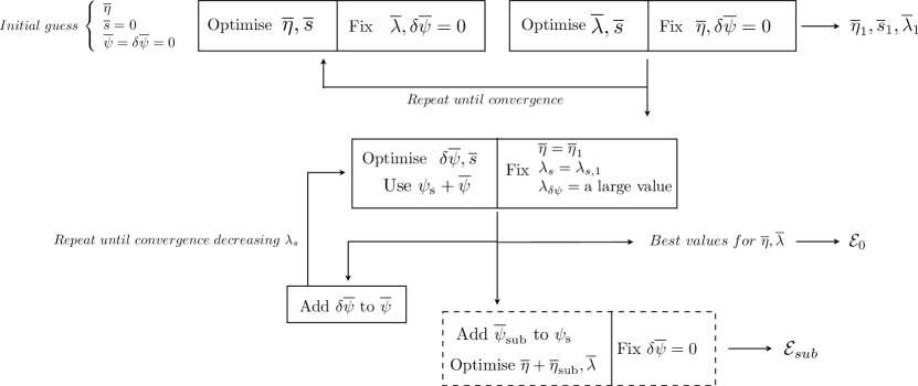
In practice, we find that the optimal strategy to minimize the penalty function is the following, in order:

(1) We set $\lambda_{\rm s}$ to a large constant value such that the source model remains relatively smooth throughout the optimization (i.e. the peak brightness of the model is a factor of a few below that of the data) and keep $\mn@boldsymbol{\psi}_{n}=\mn@boldsymbol{0}$ (see also Suyu et al. 2006; Suyu et al. 2008). We then solve for $\mn@boldsymbol{\eta}$ and $\mn@boldsymbol{s}$ that minimize the penalty function.

(2) Once the best $\mn@boldsymbol{\eta}$ and $\mn@boldsymbol{s}$ are found, a Bayesian approach is used to find the best value of $\lambda_{\rm s}$ for the source only. At this point $\mn@boldsymbol{\psi}$ is still kept equal to zero.

(3) Given the new value of $\lambda_{\rm s}$, step (1) is repeated to find improved values of $\mn@boldsymbol{\eta}$ and $\mn@boldsymbol{s}$. Since the sensitivity of $\lambda_{\rm s}$ to changes in $\mn@boldsymbol{\eta}$ is rather weak, at this point the best values of $\mn@boldsymbol{\eta}$, $\mn@boldsymbol{s}$ and $\mn@boldsymbol{\lambda}$ have been found.

(4) Next, all the above parameters are kept fixed and we solve for $\mn@boldsymbol{r}$, this time assuming a very large value for $\lambda_{\delta\psi}$ to keep the potential correction (and convergence) smooth. We adjust $\mn@boldsymbol{\psi}$ at every iteration until convergence is reached (e.g. Suyu et al. 2008). At this point we stop the optimization procedure.

(5) The smooth model with $\mn@boldsymbol{\psi}=\mn@boldsymbol{0}$ and the same model with $\mn@boldsymbol{\psi}\neq\mn@boldsymbol{0}$ are then compared through their Bayesian evidence values and errors on the parameters are estimated through the Nested Sampling of Skilling (2004)(Section 4).

Fig. 3 shows a complete flow diagram of our optimization scheme. In the next section we place equation (14) and model ranking on a formal Bayesian footing. Those readers mostly interested in the application and tests of the method could continue reading in Section 5.

Figure 3: A schematic overview of the non-linear source and potential reconstruction method.

4 A Bayesian approach to data fitting and model selection

When trying to constrain the physical properties of the lens galaxy, within the grid-based approach, three different problems are faced. Given the linear relation in equation (6) we need to determine the linear parameters $\mn@boldsymbol{r}$ for a certain set of data $\mn@boldsymbol{d}$ and a form for the smooth potential $\psi_{s}(\mn@boldsymbol{x},\mn@boldsymbol{\eta})$. We then aim to find the best values for the parameters $\mn@boldsymbol{\eta}$ and $\mn@boldsymbol{\lambda}$ and finally, on a more general level, we wish to infer the best model for the overall potential and quantitatively rank different potential families. In particular, we want to compare smooth models with models that also include a potential grid for substructure (with more free parameters). These issues can all be quantitatively and objectively addressed within the framework of Bayesian statistics. In the context of data modelling three levels of inference can be distinguished (MacKay 1992; Suyu et al. 2006).

(1) First level of inference: linear optimization. We assume the model $\mathbf{M_{c}}$, which depends on a given potential and source model, to be true and for a fixed form $\mathbf{R}$ and level ($\mn@boldsymbol{\lambda}$) of regularization, we derive from Bayes’ theorem the following expression:

$$P\left(\mn@boldsymbol{r}\,|\,\mn@boldsymbol{d},\mn@boldsymbol{\lambda},\mn@boldsymbol{\eta},\mathbf{M_{c}},\mathbf{R}\right)=\frac{P(\mn@boldsymbol{d}\,|\,\mn@boldsymbol{r},\mn@boldsymbol{\eta},\mathbf{M_{c}})\,P(\mn@boldsymbol{r}\,|\,\mn@boldsymbol{\lambda},\mathbf{R})}{P(\mn@boldsymbol{d}\,|\,\mn@boldsymbol{\lambda},\mn@boldsymbol{\eta},\mathbf{M_{c}},\mathbf{R})}\,.$$ (22)

The likelihood term, in case of Gaussian noise, for a covariance matrix $\mathbf{C_{d}}$, is given by

$$P(\mn@boldsymbol{d}\,|\,\mn@boldsymbol{r},\mn@boldsymbol{\eta},\mathbf{M_{c}})=\frac{1}{Z_{d}}\exp{[-E_{d}(\mn@boldsymbol{d}\,|\,\mn@boldsymbol{r},\mn@boldsymbol{\eta},\mathbf{M_{c}})]}\,$$ (23)

where

$$Z_{d}=(2\pi)^{N_{d}/2}(\det\ \mathbf{C_{d}})^{1/2}$$ (24)

and (see equation 15)

$$E_{d}(\mn@boldsymbol{d}\,|\,\mn@boldsymbol{r},\mn@boldsymbol{\eta},\mathbf{M_{c}}]=\frac{1}{2}\,\chi^{2}=\frac{1}{2}\left(\mathbf{M_{c}}\mn@boldsymbol{r}-\mn@boldsymbol{d}\right)^{\rm T}\mathbf{C}_{D}^{-1}\left(\mathbf{M_{c}}\mn@boldsymbol{r}-\mn@boldsymbol{d}\right)\,.$$ (25)

Because of the presence of noise and often the singularity of $\det\,(\mathbf{M_{c}^{\rm T}}\mathbf{M_{c}})$, it is not possible to simply invert the linear relation in equation (6) but an additional penalty function must be defined through the introduction of a prior probability $P(\mn@boldsymbol{r}\,|\,\mn@boldsymbol{\lambda},\mathbf{R})$ on $\mn@boldsymbol{s}$ and on $\delta\mn@boldsymbol{\psi}$. In our implementation of the method, the prior assumes a quadratic form, with minimum in $\mn@boldsymbol{r}=\mn@boldsymbol{0}$ and sets the level of smoothness (specified in $\mathbf{H}$ and $\mn@boldsymbol{\lambda}$) for the solution

$$P(\mn@boldsymbol{r}\,|\,\mn@boldsymbol{\lambda},\mathbf{R})=\frac{1}{Z_{r}}\exp{\left[-\mn@boldsymbol{\lambda}E_{r}(\mn@boldsymbol{r}\,|\,\mathbf{R})\right]}\,,$$ (26)

with

$$Z_{r}(\mn@boldsymbol{\lambda})=\int{d\mn@boldsymbol{r}e^{-\mn@boldsymbol{\lambda}E_{r}}}=e^{-\mn@boldsymbol{\lambda}E_{s}(0)}\left(\frac{2\pi}{\mn@boldsymbol{\lambda}}\right)^{N_{r}/2}(\det\mathbf{C})^{-1/2}\,,$$ (27)

$$E_{r}=\frac{1}{2}\|\mathbf{R}\mn@boldsymbol{r}\|^{2}_{2}$$ (28)

and

$$\mathbf{C}=\nabla\nabla E_{r}=\mathbf{R}\,\mathbf{R}^{\rm T}\,.$$ (29)

The normalization constant $P(\mn@boldsymbol{d}\,|\,\mn@boldsymbol{\lambda},\mn@boldsymbol{\eta},\mathbf{M_{c}},\mathbf{R})$ is called the evidence and plays an important role at higher levels of inference. In this specific case it reads

$$P(\mn@boldsymbol{d}\,|\,\mn@boldsymbol{\lambda},\mn@boldsymbol{\eta},\mathbf{M_{c}},\mathbf{R})=\frac{\int{d\mn@boldsymbol{r}\exp{(-M(\mn@boldsymbol{r}))}}}{Z_{d}Z_{r}}\,,$$ (30)

where

$$M(\mn@boldsymbol{r})=E_{d}+E_{r}\,.$$ (31)

The most probable solution for the linear parameters, is found by maximizing the posterior probability

$$P(\mn@boldsymbol{r}\,|\,\mn@boldsymbol{d},\mn@boldsymbol{\lambda},\mn@boldsymbol{\eta},\mathbf{M_{c}},\mathbf{R})=\frac{\exp(-M(\mn@boldsymbol{r}))}{\int{d\mn@boldsymbol{r}\,\exp(-M(\mn@boldsymbol{r}))}}\,.$$ (32)

The condition $\partial(E_{d}+E_{r})/\partial\mn@boldsymbol{r}=0$ now yields the set of linear equations already introduced in Section 3.1.1:

$$\left(\mathbf{M_{c}^{\rm T}}\mathbf{C_{d}}^{-1}\mathbf{M_{c}}+\mathbf{R}^{\rm T}\mathbf{R}\right)\mn@boldsymbol{r}=\mathbf{M_{c}^{\rm T}}\mathbf{C_{d}}^{-1}\mn@boldsymbol{d}\,.$$ (33)

Equation (33) is solved iteratively using a Cholesky decomposition technique.

(2) Second level of inference: non-linear optimization. At this level we want to infer the non-linear parameters $\mn@boldsymbol{\eta}$ and the hyper-parameter $\lambda_{\rm s}$ for the source. Since at this point we are interested only in the smooth component of the lens potential, we set $\delta\mn@boldsymbol{\psi}=0$ and for a fixed family $\psi_{s}(\mn@boldsymbol{\eta})$, form of the regularization $\mathbf{R}$ and model $\mathbf{M_{c}}$, we maximize the posterior probability

$$P(\mn@boldsymbol{\lambda},\mn@boldsymbol{\eta}\,|\,\mn@boldsymbol{d},\mathbf{M_{c}},\mathbf{R})=\frac{P(\mn@boldsymbol{d}\,|\,\mn@boldsymbol{\lambda},\mn@boldsymbol{\eta},\mathbf{M_{c}},\mathbf{R})P(\mn@boldsymbol{\lambda},\mn@boldsymbol{\eta})}{P(\mn@boldsymbol{d}\,|\,\mathbf{M_{c}},\mathbf{R})}\,.$$ (34)

Assuming a prior $P(\mn@boldsymbol{\lambda},\mn@boldsymbol{\eta})$, which is flat in $\log(\lambda_{s})$ and $\mn@boldsymbol{\eta}$, reduces to maximizing the evidence $P(\mn@boldsymbol{d}\,|\,\mn@boldsymbol{\lambda},\mn@boldsymbol{\eta},\mathbf{M_{c}},\mathbf{R})$ (which here plays the role of the likelihood) for $\mn@boldsymbol{\eta}$ and $\mn@boldsymbol{\lambda}$. The evidence can be computed by integrating over the posterior (34)

$$P(\mn@boldsymbol{d}\,|\,\mn@boldsymbol{\lambda},\mn@boldsymbol{\eta},\mathbf{M_{c}},\mathbf{R})=\int{d\mn@boldsymbol{r}\,P(\mn@boldsymbol{d}\,|\,\mn@boldsymbol{r},\mn@boldsymbol{\eta},\mathbf{M_{c}})P(\mn@boldsymbol{r}\,|\,\mn@boldsymbol{\lambda},\mathbf{R})}\,.$$ (35)

Because of the assumptions we made (Gaussian noise and quadratic form of regularization), this integral can be solved analytically and yields

$$P(\mn@boldsymbol{d}\,|\,\mn@boldsymbol{\lambda},\mn@boldsymbol{\eta},\mathbf{M_{c}},\mathbf{R})=\frac{Z_{M}(\mn@boldsymbol{\lambda},\mn@boldsymbol{\eta})}{Z_{d}Z_{r}(\mn@boldsymbol{\lambda})}\,,$$ (36)

where

$$Z_{M}(\mn@boldsymbol{\lambda},\mn@boldsymbol{\eta})=\exp{(-M(\mn@boldsymbol{r}_{\rm MP}))}\left(2\pi\right)^{N_{r}/2}(\det\ \mathbf{A})^{-1/2}\,,$$ (37)

with $\mathbf{A}=\nabla\nabla M(\mn@boldsymbol{r}).$ Again we proceed in an iterative fashion: using a simulated annealing technique we maximize the evidence (35) for the parameters $\mn@boldsymbol{\eta}$. Every step of the maximisation generates a new model $\mathbf{M_{c}}(\psi(\mn@boldsymbol{\eta}_{i}))$, for which the most probable source $\mn@boldsymbol{s}_{\rm{MP}}$ is reconstructed as described in Section 3. At this starting step the level of the source regularization is set to a relatively large initial value $\lambda_{s,0}$; in this way we ensure the solution to be smooth (at least at this first level) and the exploration of the $\mn@boldsymbol{\eta}$ space to be faster. Subsequently we fix the best model $\mathbf{M_{c}}(\mn@boldsymbol{\eta}_{0})$ found at the previous iteration and, using the same technique, we maximize the evidence for the source regularization level $\lambda_{s}$. The procedure is repeated until the total evidence has reached its maximum. In principle we should have built a nested loop for $\lambda_{s}$ at every step of the $\mn@boldsymbol{\eta}$ exploration, but in practice the regularization constant only changes slightly with $\mn@boldsymbol{\eta}$ and the alternate loop described above gives a faster way to reach the maximum (line-search method).

(3) At the third level of inference Bayesian statistics provides an objective and quantitative procedure for model comparison and ranking on the basis of the evidence,

$$P(\mathbf{M_{c}},\mathbf{R}\,|\,\mn@boldsymbol{d})\propto P(\mn@boldsymbol{d}\,|\,\mathbf{M_{c}},\mathbf{R})P(\mathbf{M_{c}},\mathbf{R})\,.$$ (38)

For a flat prior $P(\mathbf{M_{c}},\mathbf{R})$ (at this level of inference we can make little to no assumptions) different models can be compared according to their value of $P(\mn@boldsymbol{d}\,|\,\mathbf{M_{c}},\mathbf{R})$, which is related to the evidence of the previous level by the following relation

$$P(\mn@boldsymbol{d}\,|\,\mathbf{M_{c}},\mathbf{R})=\int{d\mn@boldsymbol{\lambda}\,d\mn@boldsymbol{\eta}\,P(\mn@boldsymbol{d}\,|\,\mn@boldsymbol{\lambda},\mn@boldsymbol{\eta},\mathbf{M_{c}},\mathbf{R})P(\mn@boldsymbol{\lambda},\mn@boldsymbol{\eta})}\,.$$ (39)

Being multidimensional and highly non-linear, the integral (39) is carried out numerically through a Nested-Sampling technique (Skilling 2004), which is described in more detail in the next section. A by-product of this method is an exploration of the posterior probability (34), allowing for error analysis of the non-linear parameters and of the evidence itself.

4.1 Model selection: smooth versus clumpy models

In the previous section we introduced the main structure of the Bayesian inference for model fitting and model selection. While parameter fitting simply determines how well a model matches the data and can be easily attained with the relatively simple analytic integrations of the first and second level of inference, model selection itself requires the highly non-linear and multidimensional integral (39) to be solved. This marginalized evidence can be used to assign probabilities to models and to reasonably establish whether the data require or allows additional parameters or not. Given two competing models $\rm M_{0}$ and $\rm M_{1}$ with relative marginalized evidence ${\cal{E}}_{0}$ and ${\cal{E}}_{1}$, the Bayes factor, $\Delta{\cal{E}}\equiv\log{\cal{E}}_{0}-\log{\cal{E}}_{1}$, quantifies how well $\rm M_{0}$ is supported by the data when compared with $\rm M_{1}$ and it automatically includes the Occam’s razor. Typically the literature suggests to weigh the Bayes factor using Jeffreys’ scale (Jeffreys 1961), which however provides only a qualitative indication: $\Delta{\cal{E}}<1$ is not significant, $1<\Delta{\cal{E}}<2.5$ is significant, $2.5<\Delta{\cal{E}}<5$ is strong and $\Delta{\cal{E}}>5$ is decisive.

In order to evaluate this marginalized evidence with a high enough accuracy we implemented the new evidence algorithm known as Nested Sampling, proposed by Skilling (2004). Specifically, we would like to compare two different models: one in which the lens potential is smooth and one in which substructures are present, with e.g. a NFW profile. While the first is defined by the non-linear parameters of the lens potential and of the source regularization only, the second also allows for three extra parameters: the mass of the substructure and its position on the lens plane (see Section 5)

4.2 Model ranking: nested sampling

Here, we provide a short description of how the Nested Sampling can be used to compute the marginalized evidence and errors on the model parameters; a more detailed one can be found in Skilling (2004). The Nested-Sampling algorithm integrates the likelihood over the prior volume by moving through thin nested likelihood surfaces. Introducing the fraction of total prior mass $X$, within which the likelihood exceeds ${\cal L^{*}}$, hence

$$X=\int_{{\cal{L}}>{\cal{L^{*}}}}{dX}\,,$$ (40)

with

$$dX=P\left(\mn@boldsymbol{\lambda},\mn@boldsymbol{\eta}\right)d\mn@boldsymbol{\lambda}\,d\mn@boldsymbol{\eta}\,,$$ (41)

the multi-dimensional integral (39) relating the likelihood $\cal{L}$ and the marginalized evidence $\cal{E}$ can be reduced to a one-dimensional integral with positive and decreasing integrand

$${\cal{E}}=\int_{0}^{1}{dX\,{\cal{L}}(X)}\,.$$ (42)

Where ${\cal L}(X)$ is the likelihood of the (possibly disjoint) iso-likelihood surface in parameter space which encloses a total prior mass of $X$. If the likelihood ${\cal{L}}_{j}={\cal{L}}(X_{j})$ can be evaluated for each of a given set of decreasing points, $0<X_{j}<X_{j-1}<....<1$, then the total evidence ${\cal{E}}$ can be obtained, for example, with the trapezoid rule, ${\cal{E}}=\sum_{j=1}^{m}{\cal{E}}_{j}=\sum_{j=1}^{m}{\frac{{\cal{L}}_{j}}{2}}\left(X_{j-1}-X_{j+1}\right)$.

The power of the method is that the values of $X_{j}$ do not have to be explicitly calculated, but can be statistically estimated. Specifically, the marginalized evidence is obtained through the following iterative scheme:

(1) the likelihood ${\cal{L}}$ is computed for N different points, called active points, which are randomly drawn from the prior volume.

(2) the point $X_{j}$ with the lowest likelihood is found and the corresponding prior volume is estimated statistically: after $j$ iterations the average volume decreases as $X_{j}/X_{j-1}=t$, where t is the expectation value of the largest of N numbers uniformly distributed between $\left(0,1\right)$.

(3) the term ${\cal{E}}_{j}=\frac{{\cal{L}}_{j}}{2}\left(X_{j-1}-X_{j+1}\right)$ is added to the current value of the total evidence;

(4) $X_{j}$ is replaced by a new point randomly distributed within the remaining prior volume and satisfying the condition ${\cal{L}}>{\cal{L}}^{*}\equiv{\cal{L}}_{j}$;

(5) the above steps are repeated until a stopping criterion is satisfied.

By climbing up the iso-likelihood surfaces, the method, in general, find and quantifies the small region in which the bulk of the evidence is located.

Different stopping criteria can be chosen. Following Skilling (2004), we stop the iteration when $j\gg\rm{N}H$, where H is minus the logarithm of that fraction of prior mass which contains the bulk of the posterior mass. In practical terms this means that the procedure should be stopped only when most of the evidence has been included. Given the areas ${\cal{E}}_{j}$, in fact, the likelihood initially increases faster than the widths decrease, until its maximum is reached; across this maximum, located in the region ${\cal{E}}\thickapprox e^{-H}$, the likelihood flatten off and the decreasing widths dominate the increasing ${\cal{L}}_{j}$. Since ${\cal{E}}_{j}\thickapprox e^{-j/\rm{N}}$, it takes $\rm{N}H$ iterations to reach the dominating areas. These $\rm{N}H$ iterations are random and are subjected to a standard deviation uncertainty $\sqrt{\rm{N}H}$, corresponding to a deviation standard on the logarithmic evidence of $\sqrt{\rm{N}H}/\rm{N}$

$${\log\cal{E}}=\log\left(\sum_{j}{{\cal{E}}_{j}}\right)\mathrm{\leavevmode\nobreak\ \leavevmode\nobreak\ \leavevmode\nobreak\ with\leavevmode\nobreak\ \leavevmode\nobreak\ \leavevmode\nobreak\ }\sigma_{\log{\cal E}}=\sqrt{\frac{H}{\rm{N}}}\,.$$ (43)

4.2.1 Posterior probability distributions

For the lens parameters, the substructure position and the logarithm of the source regularization, priors are chosen to be uniform on a symmetric interval around the best values which we have determined at the second level of the Bayesian inference. The size of the interval being at least one order of magnitude larger than the errors on the parameters. In practice, we first carry out a fast run of the Nested Sampling with few active points $\rm{N}$, this gives us an estimate for the non-linear parameter errors. Using the product $2\times N_{\rm dim}\times\sigma_{\eta}$, where $N_{\rm dim}$ is the total number of parameters and $\sigma_{\eta}$ the corresponding standard deviation, we can then roughly enclose the bulk of the likelihood (note that this can be double-checked and corrected in hindsight, if the posterior probability functions are truncated at the prior boundaries). Priors on the parameters are taken in such a way that this maximum is fully included in the total integral of the marginalized evidence. For the main lens parameters and for the regularization constant the same priors are used for model with and without substructure. For the substructure mass a flat prior between $M_{\rm min}=4.0\times 10^{6}M_{\odot}$ and $M_{\rm max}=4.0\times 10^{9}M_{\odot}$ is adopted, with the two limits given by N-body simulations (e.g. Diemand et al. 2007a, b). In reality, the method does not require the parameters to be well known a priori, but limiting the exploration to the best fit region sensibly reduces the computational effort without significantly altering the evidence estimation. From Bayes theorem we have that the posterior probability density $p_{j}$ is given by

$$p_{j}(t)=\frac{{\cal{L}}_{j}}{2}\left(X_{j-1}-X_{j+1}\right)/{\cal{E}}(t)=w_{j}/{\cal{E}}(t)\,.$$ (44)

The existing set of points $\left(\mn@boldsymbol{\eta},\mn@boldsymbol{\lambda}\right)_{1}$,…, $\left(\mn@boldsymbol{\eta},\mn@boldsymbol{\lambda}\right)_{\rm N}$ then gives us a set of posterior values that can be then used to obtain mean values and standard deviations on the non-linear parameters

$$\langle\mn@boldsymbol{\eta}\rangle=\sum_{j}{w_{j}\mn@boldsymbol{\eta}_{j}}/\sum_{j}{w_{j}}\,,$$ (45)

and similarly for $\mn@boldsymbol{\lambda}$. These samples also provide a sampling of the full joint probability density function. Marginalising over this function, the full marginalized probability density distribution of each parameters can be determined (see Section 5.5).

5 Testing and calibrating the method

In this section we describe the procedure to test the method introduced above and to assess its ability to detect dark matter substructures in realistic data sets (e.g. from HST). A set of mock data, mimicking a typical Einstein ring, is created. We generate fourteen different lens models, of which $\rm L_{0}$ is purely smooth, $\rm L_{1\leq i<13}$ are given by the superposition of the same smooth potential with a single NFW dark matter substructure of varying mass and position and $\rm L_{13}$ contains two NFW dark matter substructures with the same mass but with different positions (See Table 1). A first approximate reconstruction of the source and of the lens potential is performed by recovering the best non-linear lens parameters $\mn@boldsymbol{\eta}$ and the level of source regularization $\lambda_{s}$. These values are then used for the linear grid-based optimization, which provides initial values of the substructure position and mass. Three extra runs of the non-linear optimization are then performed to recover the best set $\left(\mn@boldsymbol{\eta}_{b},\lambda_{s,b}\right)$ for the main lens and the best mass and position of the substructure (solely modelled with a NFW density profile). Finally by means of the Nested-Sampling technique described in Section 4.1 we compute the marginalized evidence, equation (39), for every model twice, once under the hypothesis of a smooth lens and once allowing for the presence of one or two extra mass substructures. Comparison between these two models allows us to assess whether the presence of substructure in the model improves the evidence despite the larger number of free parameters.

5.1 Mock data realisations

A set of simulated data with realistic noise is generated from a model based on the real lens SLACS J1627$-$0055 (Koopmans et al. 2006; Bolton et al. 2006; Treu et al. 2006). We assume the lens to be well described by a power-law (PL) profile (Barkana 1998). Using the optimization technique described in Section (4) we find the best set of non-linear parameters $\left(\mn@boldsymbol{\eta}_{b},\lambda_{s,b}\right)$. In particular $\mn@boldsymbol{\eta}$ contains the lens strength $b$, and some of the lens-geometry parameters: the position angle $\theta$, the axis ratio $f$, the centre coordinates $\mn@boldsymbol{x}_{0}$ and the density profile slope $q$, $\left(\rho\propto r^{-(2q+1)}\right)$. If necessary, information about external shear can be included. The best parameters are used to create fourteen different lenses and their corresponding lensed images. One of the systems is given by a smooth PL model while twelve include a dark matter substructure with virial mass $\rm M_{vir}=10^{7}\rm M_{\odot},10^{8}\rm M_{\odot},10^{9}\rm M_{\odot}$ located either on the lowest surface brightness point of the ring $P_{0}$, on a high surface brightness point of the ring $P_{1}$, inside the ring $P_{2}$ and outside the ring $P_{3}$ (see Table 1). The fourteenth lens contains two substructures each with a mass of $\rm M_{vir}=10^{8}M_{\odot}$, located respectively in $P_{0}$ and $P_{1}$. The substructures are assumed to have a NFW profile

$$\rho\left(r\right)={\rho_{s}}{\left(r_{s}/r\right)\left[1+\left(r/r_{s}\right)\right]^{-2}}\,,$$ (46)

where the concentration $c=r_{\mathrm{vir}}/r_{s}$ and the scaling radius $r_{s}$ are obtained from the virial mass using the empirical scaling laws provided by Diemand et al. (2007a, b). The source has an elliptical Gaussian surface brightness profile centred in zero

$$s\left(\mn@boldsymbol{y}\right)=s_{0}\exp\left[-(y_{1}/\delta y_{1})^{2}-(y_{2}/\delta y_{2})^{2}\right]\,.$$ (47)

We assume $s_{0}=0.25$, $\delta y_{1}=0.01$ and $\delta y_{2}=0.04$.

Table 1: Non-smooth (PL+NFW) lens models. At each of the $P_{i}$ positions a NFW perturbation of virial mass $m_{sub}$ is superimposed on a smooth PL mass model distribution.

Lens	$\mn@boldsymbol{x}_{sub}$ $\left(\mathrm{arcsec}\right)$	$m_{sub}$ $\left(M_{\odot}\right)$
$\rm L_{1}$	$P_{0}=(+0.90;+1.19)$	$10^{7}$
$\rm L_{2}$		$10^{8}$
$\rm L_{3}$		$10^{9}$
$\rm L_{4}$	$P_{1}=(-0.50;-1.00)$	$10^{7}$
$\rm L_{5}$		$10^{8}$
$\rm L_{6}$		$10^{9}$
$\rm L_{7}$	$P_{2}=(-0.10;-0.60)$	$10^{7}$
$\rm L_{8}$		$10^{8}$
$\rm L_{9}$		$10^{9}$
$\rm L_{10}$	$P_{3}=(-0.90;-1.40)$	$10^{7}$
$\rm L_{11}$		$10^{8}$
$\rm L_{12}$		$10^{9}$
$\rm L_{13}$	$P_{0}$ and $P_{1}$	$10^{8}$

5.2 Non-linear reconstruction of the main lens

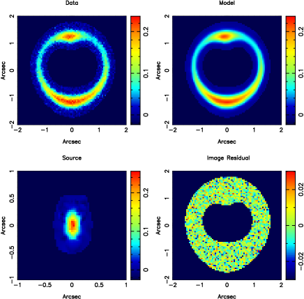
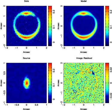
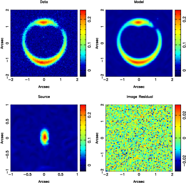
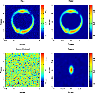
We start by choosing an initial parameter set $\mn@boldsymbol{\eta}_{0}$ for the main lens, which is offset from $\mn@boldsymbol{\eta}_{\rm true}$ that we used to create the simulated data. Assuming the lens does not contain any substructure we run the non-linear procedure described in Section (4) and optimize $\{\mn@boldsymbol{\eta},\lambda_{s}\}$ for each of the considered systems. At every step of the optimization a new set $\{\mn@boldsymbol{\eta}_{i},\lambda_{s,i}\}$ is obtained and the corresponding lensing operator $\mathbf{M_{c}}(\mn@boldsymbol{\eta}_{i},\lambda_{s,i})$ has to be re-computed. The images are defined on a 81 by 81 pixels $\left(N_{d}=6561\right)$ regular Cartesian grid while the sources are reconstructed on a Delaunay tessellation grid of $N_{s}=441$ vertices. The number of image points, used for the source grid construction, is effectively a form of a prior and the marginalized evidence (equation 39) can be used to test this choice. To check whether the number of image pixels used can affect the result of our modelling, we consider the smooth lens $\rm L_{0}$ and perform the non-linear reconstruction using one pixel every sixteen, nine, four and one. In each of the considered cases we find that the lens parameters are within the relative errors (see Table  3). This suggests that, for this particular case, the choice of number of pixels is not influencing the quality of the reconstruction. In real systems, the dynamic range of the lensed images could be much higher and a case by case choice based on the marginalized evidence has to be considered. In Fig. 5, the residuals relative to the system $\rm L_{1}$ are shown; the noise level is in general reached and only small residuals are observed at the position of the substructure. Whether the level of such residuals and therefore the relative detection of the substructure are significant is an issue we will address later on in terms of the total marginalized evidence.

5.3 Linear reconstruction: substructure detection

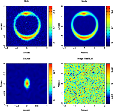
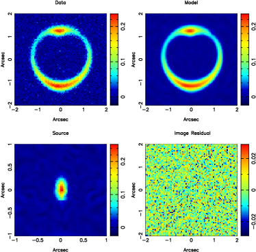
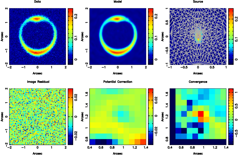
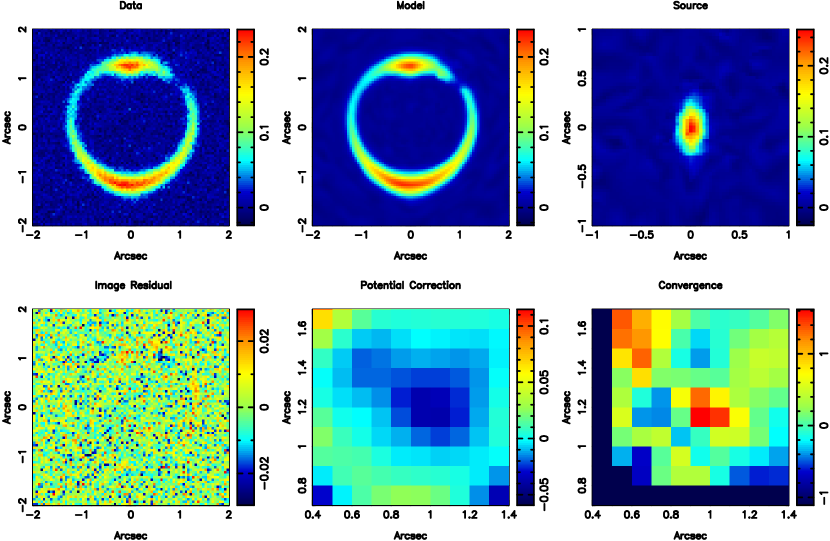
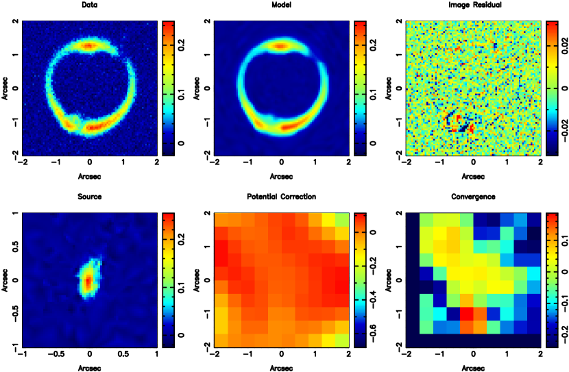
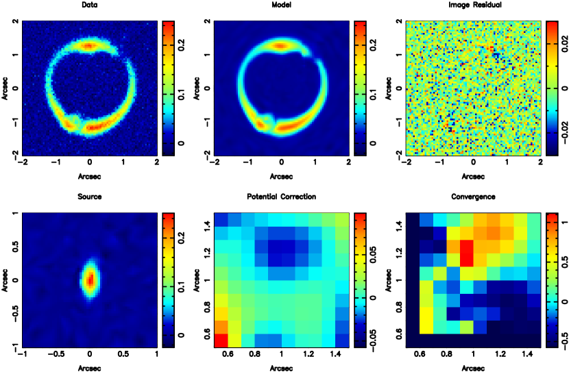
The non-linear optimization provides us with a first good approximate solution for the source and for the smooth component of the lens potential. While this is a good description for the smooth model $\rm L_{0}$ (see Fig. 4), the residuals (e.g. Fig. 7) for the perturbed model $\rm L_{i\geq 1}$ indicate that the no-substructure hypothesis is improbable and that perturbations to the main potential have to be considered. If the perturbation is small, this can be done by temporarily assuming that $\mn@boldsymbol{\eta}_{i=1}$ reflects the true mass model distribution for the main lens and reconstruct the source and the potential correction by means of equation (33). In order to keep the potential corrections in the linear regime, where the approximation (33) is valid, both the source and the potential need to be initially over-regularised: $\lambda_{s}=10\,\lambda_{s,1}$ and $\lambda_{\delta\psi}=3.0\times 10^{5}$ (Koopmans 2005; Suyu et al. 2006). For each of the possible substructure positions we identify the lowest-mass-substructure we are able to recover. In the two most favourable cases, $\rm L_{1}$ and $\rm L_{4}$, in which the substructure sits on the Einstein ring a perturbation of $10^{7}\rm M_{\odot}$ is readily reconstructed. For these two positions higher mass models, with the exception of $\rm L_{2}$, will not be further analysed. The systems $\rm L_{7,8,9}$ and $\rm L_{10,11,12}$, in which the substructure is located, respectively, inside and outside the ring, represent more difficult scenarios. In the first case all perturbations below $10^{9}\rm M_{\odot}$ can be mimicked by an increase of the mass of the main lens within the ring, while in the second case these cannot be easily distinguished from an external shear effect. For the models $\rm L_{1,2,4,9,12}$ convergence is reached after 150 iterations and the perturbations are recovered near their known position (Figs. 8 and 9). The grid based potential reconstruction indeed leads to a good first estimation for the substructure position.

5.4 Non-linear reconstruction: main lens and substructure

In order to compare with numerical simulations, the mass of the substructure is required. Performing this evaluation with a grid based reconstruction is more complicated and requires some assumptions (e.g. aperture). To alleviate this problem we assume a parametric model, in which the substructures are described by a NFW density profile, and we recover the corresponding non-linear parameters, mass and position, using the non-linear Bayesian optimization previously described.

To quantify the mass and position of the substructure and to update the non-linear parameters when a substructure is added, we adopt a multi-step non-linear procedure that relatively fast converges to a best PL+NFW mass model. At this level, we neglect the smooth lens $\rm L_{0}$, for which a satisfactory model already has been obtained after the first non-linear optimization, and the perturbed models $\rm L_{7,8,10,11}$ for which the substructure could not be recovered. We proceed as follows:

(i) we fix the main lens parameters to the best values found in Section (5.3), $\{\mn@boldsymbol{\eta}_{1},\lambda_{\rm s,1}\}$. We set the substructure mass to some guess value. We optimize for the substructure position $\mn@boldsymbol{x}_{\rm sub,1}$.

(ii) we fix $\{\mn@boldsymbol{\eta}_{1},\lambda_{s,1}\}$ and the source position $\mn@boldsymbol{x}_{\rm sub,1}$. We optimize for the substructure mass $m_{\rm sub,1}$.

(iii) we run the non-linear procedure described in Section (4) by alternatively optimising for the main lens, source, and substructure parameters and for the level of source regularization.

This leads to a new set of parameters, $\{\mn@boldsymbol{\eta}_{\rm b},\lambda_{\rm s,b},m_{\rm sub,b},\mn@boldsymbol{x}_{\rm sub,b}\}$. Final results for the considered models are listed in Table 3 and the relative residuals are shown in the Figs. 5-7, respectively. For all the considered lenses the final reconstruction converges to the noise level.

5.5 Multiple substructures

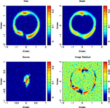
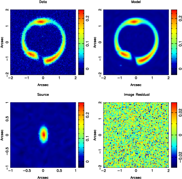
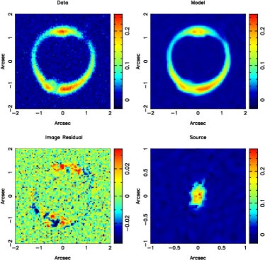
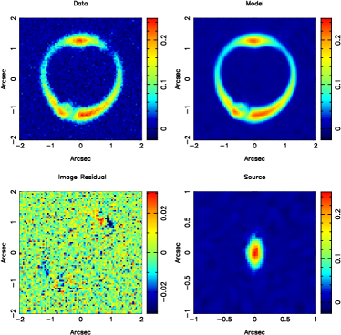
The lens system $\rm L_{13}$ represents a more complex case in which two substructures are included. In particular we are interested in testing whether both substructures are detectable and whether their effect may be hidden by the presence of external shear. As for the previously considered cases, we first perform a non-linear reconstruction of the main lens parameters assuming a single PL mass model. For this particular system we also include the strength $\rm\Gamma_{sh}$ and the position angle $\rm\theta_{sh}$ of the external shear as free parameters. Results for this first step of the reconstruction are shown in Fig. 10. We then run the linear potential reconstruction. One of the two substructures is detected although a significant level of image residuals is left (Fig. 11). The combined effect of external shears ($\rm\Gamma_{sh}=-0.031$) and the substructure in $P_{1}$ is not sufficient to explain the perturbation generated by the second substructure at the lowest surface brightness point of the Einstein ring. We therefore include a NFW substructure in the recovered position and run a non-linear reconstruction for the new PL+NFW model, Fig. 10. We are then able to detect also the second substructure, Fig. 12. Finally we run a global non-linear reconstruction for the PL+2NFW model (Fig. 10), the noise level is reached and the strength of the external shear is consistent with zero ($\rm\Gamma_{sh}=0.0001$).

5.6 Nested sampling: the evidence for substructure

When modelling systems as $\rm L_{0}$ or $\rm L_{i\geq 1}$ we assume that the best recovered values, under the hypothesis of a single power-law, provide a good description of the true mass distribution and that any eventually observed residual could be an indication for the presence of mass substructure. Model comparison within the framework of Bayesian statistics gives us the possibility to test this assumption.

5.6.1 Marginalized Bayesian evidence

In order to statistically compare two models the marginalized evidence (39) has to be computed. As described in Section (4.1) this multi-dimensional and non-linear integral can be evaluated using the Nested-Sampling technique by Skilling (2004). Specifically the two mass models we wish to compare are a single PL, M₀, versus a PL+NWF substructure, M₁. The first one is completely defined by the non-linear parameters $\left(\mn@boldsymbol{\eta},\lambda_{s}\right)$, while the second needs three extra parameters, namely the substructure mass and position. For all these parameters prior probabilities have to be defined:

$$P\left(\eta_{i}\right)=\left\{\begin{array}[]{ll}\text{constant}&{\rm\leavevmode\nobreak\ \leavevmode\nobreak\ \leavevmode\nobreak\ for\leavevmode\nobreak\ \leavevmode\nobreak\ \leavevmode\nobreak\ }|\eta_{\rm{b},i}-\eta_{i}|\leq\delta\eta_{i}\\ &\\ 0&{\rm\leavevmode\nobreak\ \leavevmode\nobreak\ \leavevmode\nobreak\ for\leavevmode\nobreak\ \leavevmode\nobreak\ \leavevmode\nobreak\ }|\eta_{\rm{b},i}-\eta_{i}|>\delta\eta_{i}\end{array}\right.$$ (48)

and

$$P\left(x_{\rm{sub},i}\right)=\left\{\begin{array}[]{ll}\text{constant}&{\rm\leavevmode\nobreak\ \leavevmode\nobreak\ \leavevmode\nobreak\ for\leavevmode\nobreak\ \leavevmode\nobreak\ \leavevmode\nobreak\ }|x_{\rm{sub,b},i}-x_{\rm{sub},i}|\leq\delta x_{\rm{sub},i}\\ &\\ 0&{\rm\leavevmode\nobreak\ \leavevmode\nobreak\ \leavevmode\nobreak\ for\leavevmode\nobreak\ \leavevmode\nobreak\ \leavevmode\nobreak\ }|x_{\rm{sub,b},i}-x_{\rm{sub},i}|>\delta x_{\rm{sub},i}\end{array}\right.$$ (49)

where the elements of $\delta\eta_{i}$ and $\delta x_{\rm sub,i}$ are empirically assessed such that the bulk of the evidence likelihood is included (see Skilling 2004). The prior on the substructure mass is flat between the lower and upper mass limits given by numerical simulations (e.g. Diemand et al. 2007a, b). Given the lenses $\rm L_{0,1,2,4,9,12,13}$ we run the Nested Sampling twice, once for the single PL model and once for the PL+NFW (+NFW) one. The two marginalized evidences with corresponding numerical errors can be compared from Table  2. Despite a certain number of authors suggest the use of Jeffreys’ scale (Jeffreys 1961) for model comparison, we adopt here a more conservative criterion. In particular, we note that the perturbed model M₁ for the lens system $\rm L_{0}$ is basically consistent with a single smooth PL model M₀, with $\Delta{\cal{E}}\sim 7.85$. The Bayesian factor for the system $\rm L_{4}$ is of the order of $\Delta{\cal{E}}\sim 21.5$ in favour of the smooth model M₀, indicating that the detection of such a low-mass substructure can formally not be claimed at a significant level. The reason why we think this substructure is clearly visible in the grid-based results, is that this particular solution is the maximum-posterior (MP) solution, whereas the evidence gives the integral over the entire parameter space. This implies that there must be many solutions near the MP solution that do not show the substructure. This indicates that our approach of quantifying the evidence for substructure is very conservative. On the other hand the Bayes factor for the lens $\rm L_{1}$, $\Delta{\cal{E}}=-17.1$, clearly shows that the detection of a $10^{7}M_{\odot}$ substructure can be significant when the latter is located at a different position on the ring. Finally all higher mass perturbations are easily detectable independently of their position relative to the image ring; Bayes factor for $\rm L_{2}$, $\rm L_{9}$, $\rm L_{12}$ and $\rm L_{13}$ are, in fact, respectively $\Delta{\cal{E}}=-213.0$, $\Delta{\cal{E}}=-2609.7$, $\Delta{\cal{E}}=-4603.4$ and $\Delta{\cal{E}}=-1835.7$. Substructure properties for these systems are also confidently recovered. The main difference between Jeffreys’ scale and our criterion for quantifying the significance level of the substructure detection is observed for the system $\rm L_{1}$. If we had to adopt Jeffreys’ scale in fact, such detection would have to be claimed decisive while we think it is only significant.

Figure 4: Results of the non-linear optimization for the smooth lens $\rm{L_{0}}$. The top-right panel shows the original mock data, while the top-left one shows the final reconstruction. On the second row the source reconstruction (left) and the image residuals (right) are shown.

5.7 Posterior probabilities

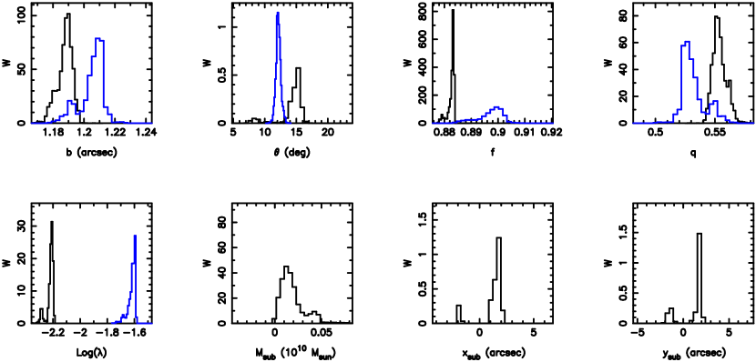
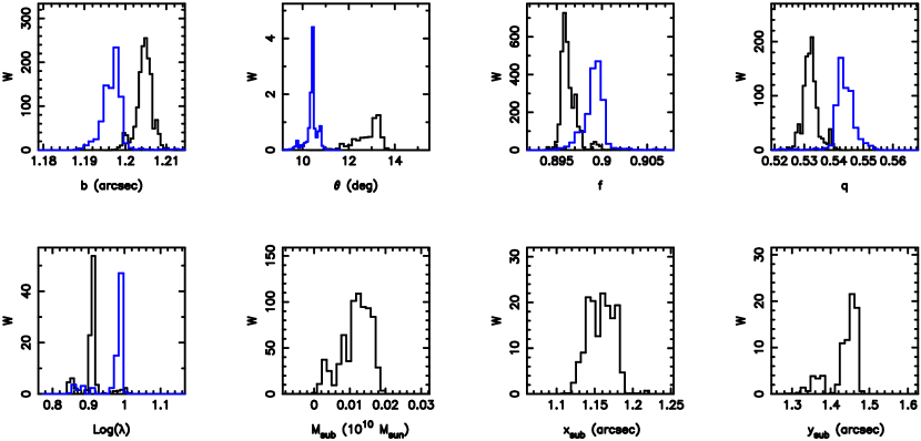
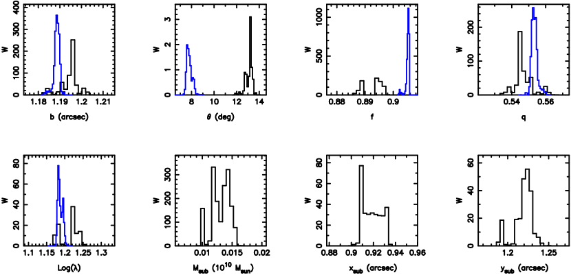
As discussed in Section (4.1) an interesting by-product of the Nested-Sampling procedure is an exploration of the posterior probability (34) which provides us with statistical errors on the model parameters, see Tables 3 and 4. The relative posterior probabilities for $\rm L_{0}$, $\rm L_{1}$ and $\rm L_{2}$ are plotted in Fig. 13, Fig. 14 and Fig. 15 respectively. Lets start by considering the lens system $\rm L_{0}$ and the relative probability distribution for the substructure mass. Although the model M₁, in terms of marginalized evidence, is consistent with the single smooth PL model M₀, there is a small probability for the presence of a substructure with mass up to few $10^{8}M_{\odot}$ located as far as possible from the ring. The effect of such objects on the lensed image would be very small and could be easily hidden by introducing artificial features in the source structure, as suggested by the posterior distributions for the source regularization constant. This means, that from the image point of view, a smooth single PL model and a perturbed PL+NWF with a substructure of $10^{8}M_{\odot}$, located far from ring, are not distinguishable from each other as long as the effect of the perburber can be hidden in the structure of the source. From a probabilistic point of view, however, the second scenario is more unlikely to happen. A similar argument can be applied to the lens $\rm L_{1}$ for which a strong degeneracy between the mass and the position of the substructure is observed. We conclude therefore that, although this substructure can be detected at a statistically significant level, its mass and position cannot be confidently assessed yet. In contrast, for systems such as $\rm L_{2,9,12}$, the effect of the substructure is so strong that it can not be mimicked by the source structure or by a different combination of the substructure parameters. For these cases not only the detection is highly significant, but the properties of the perturber can be confidently constrained with minimal biases.

Table 2: marginalized evidence and corresponding standard deviation as obtained via the Nested-Sampling integration. Results are shown for the hypothesis of a smooth lens (PL) and the hypothesis of a clumpy lens potential (PL+NFW).

Lens	Model	$\log{\cal E}\,$	$\sigma_{{\log{\cal E}}}\,$
$\rm L_{0}$	PL	26332.70	0.33
	PL+NFW	26324.85	0.30
$\rm L_{1}$	PL	20366.86	0.34
	PL+NFW	20383.95	0.30
$\rm L_{4}$	PL	20292.40	0.33
	PL+NFW	20270.87	0.29
$\rm L_{9}$	PL	17669.41	0.45
	PL+NFW	20279.13	0.36
$\rm L_{12}$	PL	15786.91	0.33
	PL+NFW	20390.35	0.37
$\rm L_{13}$	PL	18509.76	0.24
	PL+2 NFW	20346.48	0.49

Figure 5: Left panel: Results of the first non-linear reconstruction for the smooth component of the perturbed lens L₁. The top-right panel shows the original mock data, while the top-left one shows the final reconstruction. On the second row the source reconstruction (left) and the image residuals (right) are shown. Right panel: Final results of the non-linear reconstruction for the perturbed lens L₁. The top-right panel shows the original mock data, while the top-left one shows the final model reconstruction obtained after a non-linear optimization involving the lens parameters and the substructure position and mass. The recovered source is plotted in the low-left panel. Image residuals (right) are shown.

Figure 6: Similar as Figure 5 for L₂.

6 Conclusions and Future work

We have introduced a fully Bayesian adaptive method for objectively detecting mass substructure in gravitational lens galaxies. The implemented method has the following specific features:

• Arbitrary imaging data-set defined on a regular grid can be modelled, as long as only lensed structure is included. The code is specifically tailored to high-resolution HST data-sets with a compact PSF that can be sampled by a small number of pixels.

• Different parametric two-dimensional mass-models can be used, with a set of free parameter $\mn@boldsymbol{\eta}$. Currently, we have implemented the elliptical power-law density models from Barkana (1998), but other models can easily be included. Multiple parametric mass models can be simultaneously optimized.

• A grid-based correction to the parametric potential can iteratively be determined for any perturbation that can not easily be modelled within the chosen family of potential models (e.g. warps, twists, mass-substructures, etc.).

• The source surface-brightness structure is determined on a fully adaptive Delaunay tessellation grid, which is updated with every change of the lens potential.

• Both model-parameter optimization and model ranking are fully embedded in a Bayesian framework. The method takes special care not to change the number of degrees of freedom during the optimization, which is ensured by the adaptive source grid. Methods with a fixed source surface-brightness grid can not do this.

• Both source and potential solutions are regularised, based on a smoothness criterion. The choice of regularization can be modified and the level of regularization is set by Bayesian optimization of the evidence. The data itself determine what level of regularization is needed. Hence overly smooth or overly irregular structure is automatically penalised.

• The maximum-posterior and the full marginalized probability distribution function of all linear and non-linear parameters can be determined, marginalized over all other parameters (including regularization). Hence a full exploration of all uncertainties of the model is undertaken.

• The full marginalized evidence (i.e. the probability of the model given the data) is calculated, which can be used to rank any set of model assumptions (e.g. pixel size, PSF) or model families. In our case, we intend to compare smooth models with models that include mass substructure. The marginalized evidence implicitly includes Occam’s razor and can be used to assess whether substructure or any other assumption is justified, compared to a null-hypothesis.

The method has been tested and calibrated on a set of artificial but realistic lens systems, based on the lens system SLACS J1627$-$0055.

The ensemble of mock data consists of a smooth PL lens and thirteen clumpy models including one or two NFW substructures. Different values for the mass and the substructure position have been considered. Using the Bayesian optimization strategy developed in this paper we are able to recover the smooth PL system and all perturbed models with a substructure mass $\ga 10^{7}M_{\odot}$ when located at the lowest surface brightness point on the Einstein ring and with a mass $\geq 10^{9}M_{\odot}$ when located just inside or outside the ring (i.e. their Einstein rings need to overlap roughly). For all these models we have convincingly recovered the best set of non-linear parameters describing the lens potential and objectively set the level of regularization.

Furthermore, our implementation of the Nested-Sampling technique provides statistical errors for all model parameters and allows us to objectively rank and compare different potential models in terms of Bayesian evidence, removing as much as possible any subjective choices. Any choice can quantitatively be ranked. For each of the lens systems we compare a complete smooth PL mass model with a perturbed PL+NFW (+NFW) one. The method here developed allows us to solve simultaneously for the lens potential and the lensed source. The latter, in particular, is reconstructed on an adaptive grid which is re-computed at every step of the optimization, allowing to take into account the correct number of degrees of freedom.

Figure 7: Similar as Figure 5 for L₁₂.

Figure 8: Results of the linear source and potential reconstruction for the lens L₁. The first row shows the original model (left), the reconstructed model (middle) and the current-best source, as well as the corresponding adaptive grid. On the second row the image residuals (left), the total potential convergence (middle) and the substructure convergence (right) are shown. Note that the substructure, although weak, is reconstructed at the correct position.

Figure 9: Similar as Figure 8 for L₂. We note that the substructure is extremely well reconstructed, both at the correct position and in mass.

Figure 10: Non linear reconstruction of the lens $\rm L_{13}$ for a single PL model, a PL+NFW and a PL+2NFW one.

Figure 11: Results of the first linear source and potential reconstruction for the lens L₁₃. The first row shows the original model (left), the reconstructed model (middle) and the image residuals. On the second row the current-best source (left), the total potential convergence (middle) and the substructure convergence (right) are shown. Note that the substructure, although weak, is reconstructed at the correct position.

Figure 12: Results of the second linear source and potential reconstruction for the lens L₁₃.

In this paper we have considered systems which contains at most two CDM substructures. Although it may appear as a very small number when compared with predictions from N-body simulations within the virial radius, this represents a realistic scenario. As we have shown, our method, with current HST data, is mostly sensitive to perturbations with mass $\ga 10^{7}\rm M_{\odot}$ and located on the Einstein ring ($\Delta\theta\sim\mu\theta_{\rm ER}$). The projected volume that we are able to probe is therefore small compared to the projected volume within the virial radius. The probability that more than two substructures have this right combination of mass and position is relatively low and we expect most of the real systems to be dominated by one or at most two perturbers. Despite these new results, further improvements can still be made. We think, for example, that an adaptive source grid based on surface brightness, rather than magnification, or a combination, could be more suitable for the scientific problem considered here.

The method will soon be applied to real systems, as for example from the Sloan Lens ACS Survey sample of massive early-type galaxies (Koopmans et al. 2006; Bolton et al. 2006; Treu et al. 2006). This will lead to powerful new constraints or limits on the fraction and mass distribution of substructure. Results will be compared with CDM simulations.

Figure 13: Posterior probability distributions for the non linear parameters of the smooth lens model $\rm L_{0}$ as obtained from the Nested-Sampling evidence exploration. In particular results for two different models are shown, a smooth PL potential (blue histograms) and a perturbed PL+NFW lens (black histograms). From up left, the lens strength, the position angle, the axis ratio, the slope, the logarithm of the source regularization constant, the substructure mass and position are plotted.

Figure 14: Similar as Figure 13 for L₁.

Figure 15: Similar as Figure 13 for L₂.

References

- Barkana (1998) Barkana R., 1998, ApJ, 502, 531
- Barnabè & Koopmans (2007) Barnabè M., Koopmans L. V. E., 2007, ApJ, 666, 726
- Barnes (1992) Barnes J., 1992, ApJ, 393, 484
- Bergström et al. (1999) Bergström L., Edsjö J., Gondolo P., Ullio P., 1999, Phys. Rev. D, 59, 043506
- Binney & Evans (2001) Binney J., Evans N. W., 2001, MNRAS, 327, L27
- Blandford & Narayan (1986) Blandford R., Narayan R., 1986, ApJ, 310, 568
- Bolton et al. (2006) Bolton A. S., Burles S., Koopmans L. V. E., Treu T., Moustakas L. A., 2006, ApJ, 638, 703
- Bradač et al. (2004) Bradač M., Schneider P., Lombardi M., Steinmetz M., Koopmans L. V. E., Navarro J. F., 2004, A&A, 423, 797
- Bradač et al. (2002) Bradač M., Schneider P., Steinmetz M., Lombardi M., King L. J., Porcas R., 2002, A&A, 388, 373
- Brewer & Lewis (2006) Brewer B. J., Lewis G. F., 2006, ApJ, 637, 608
- Bullock et al. (2000) Bullock J. S., Kravtsov A. V., Weinberg D. H., 2000, ApJ, 539, 517
- Burkert (1995) Burkert A., 1995, ApJ, 447, L25
- Burles et al. (2001) Burles S., Nollett K. M., Turner M. S., 2001, Phys. Rev. D, 63, 063512
- Calcáneo-Roldán & Moore (2000) Calcáneo-Roldán C., Moore B., 2000, Phys. Rev. D, 62, 123005
- Cen (2001) Cen R., 2001, ApJ, 546, L77
- Chen et al. (2007) Chen J., Rozo E., Dalal N., Taylor J. E., 2007, ApJ, 659, 52
- Chiba (2002) Chiba M., 2002, ApJ, 565, 17
- Colafrancesco et al. (2006) Colafrancesco S., Profumo S., Ullio P., 2006, A&A, 455, 21
- Cole et al. (2000) Cole S., Lacey C. G., Baugh C. M., Frenk C. S., 2000, MNRAS, 319, 168
- Colin et al. (2000) Colin P., Avila-Reese V., Valenzuela O., 2000, ApJ, 542, 622
- Croft et al. (2002) Croft R. A. C., Weinberg D. H., Bolte M., Burles S., Hernquist L., Katz N., Kirkman D. andTytler D., 2002, ApJ, 581, 20
- Dalal & Kochanek (2002) Dalal N., Kochanek C. S., 2002, ApJ, 572, 25
- de Bernardis et al. (2002) de Bernardis P., et al., 2002, ApJ, 564, 559
- de Blok & Bosma (2002) de Blok W. J. G., Bosma A., 2002, A&A, 358, 816
- de Blok et al. (2001) de Blok W. J. G., McGaugh S. S., Rubin V. C., 2001, AJ, 122, 2396
- Diemand et al. (2007a) Diemand J., Kuhlen M., Madau P., 2007a, ApJ, 667, 859
- Diemand et al. (2007b) Diemand J., Kuhlen M., Madau P., 2007b, ApJ, 657, 262
- Dye & Warren (2005) Dye S., Warren S. J., 2005, ApJ, 623, 31
- Efstathiou et al. (2002) Efstathiou G. P., et al., 2002, MNRAS, 330, L29
- Frenk et al. (1988) Frenk C. S., White S. D. M., Davis M., Efstathiou G. P., 1988, ApJ, 327, 507
- Goodman (2000) Goodman J., 2000, New Astron., 5, 103
- Hamilton & Tegmark (2002) Hamilton A. J. S., Tegmark M., 2002, MNRAS, 330, 506
- Ibata et al. (2002) Ibata R. A., Lewis G. F., Irwin M. J., Quinn T., 2002, MNRAS, 332, 915
- Jaffe et al. (2001) Jaffe A. H., et al., 2001, Phys. Rev. Lett., 86, 3475
- Jeffreys (1961) Jeffreys H., 1961, Theory of Probability. 3rd edn. Oxford Univ. Press, Oxford
- Kamionkowski & Liddle (2000) Kamionkowski M., Liddle A., 2000, Phys. Rev. Lett., 84, 4525
- Kauffmann et al. (1993) Kauffmann G., White S. D. M., Guiderdoni B., 1993, MNRAS, 264, 201
- Keeton et al. (2003) Keeton C. R., Gaudi B. S., Petters A. O., 2003, ApJ, 598, 138
- Keeton et al. (2005) Keeton C. R., Gaudi B. S., Petters A. O., 2005, ApJ, 635, 35
- Klypin et al. (1999) Klypin A., Kravtsov A. V., Valenzuela O., Prada F., 1999, ApJ, 522, 82
- Kochanek & Dalal (2004) Kochanek C. S., Dalal N., 2004, ApJ, 610, 69
- Komatsu et al. (2008) Komatsu E., et al., 2008, ApJS, preprint (arXiv:0803.0547)
- Koopmans (2005) Koopmans L. V. E., 2005, MNRAS, 363, 1136
- Koopmans & Treu (2002) Koopmans L. V. E., Treu T., 2002, ApJ, 568, L5
- Koopmans et al. (2006) Koopmans L. V. E., Treu T., Bolton A. S., Burles S., Moustakas L. A., 2006, ApJ, 649, 599
- Kravtsov et al. (2004) Kravtsov A. V., Gnedin O. Y., Klypin A. A., 2004, ApJ, 609, 482
- Kuzio de Naray et al. (2006) Kuzio de Naray R., McGaugh S. S., de Blok W. J. G., Bosma A., 2006, ApJS, 165, 461
- Macciò & Miranda (2006) Macciò A. V., Miranda M., 2006, MNRAS, 368, 599
- McGaugh et al. (2003) McGaugh S. S., Barker M. K., de Blok W. J. G., 2003, ApJ, 584, 566
- McGaugh & de Blok (1998) McGaugh S. S., de Blok W. J. G., 1998, ApJ, 499, 41
- MacKay (1992) MacKay D. J. C., 1992, PhD thesis, Caltech
- MacKay (2003) MacKay D. J. C., 2003, Information Theory, Inference and Learning Algorithms. Cambridge Univ. Press, Cambridge
- McKean et al. (2007) McKean J. P., Koopmans L. V. E., Flack C. E., Fassnacht C. D., Thompson D., Matthews K., Blandford R. D., Readhead A. . C. S., Soifer B. T., 2007, MNRAS, 378, 109
- Mao et al. (2004) Mao S., Jing Y., Ostriker J. P., Weller J., 2004, ApJ, 604, L5
- Mao & Schneider (1998) Mao S., Schneider P., 1998, MNRAS, 295, 587
- Mayer et al. (2002) Mayer L., Moore B., Quinn T., Governato F., Stadel J., 2002, MNRAS, 336, 119
- Metcalf & Zhao (2002) Metcalf R. B., Zhao H., 2002, ApJ, 567, L5
- Moore (1994) Moore B., 1994, Nature, 370, 629
- Moore et al. (2001) Moore B., Calcáneo-Roldán C., Stadel J., Quinn T., Lake G., Ghigna S., Governato F., 2001, Phys. Rev. D, 64, 063508
- Moore et al. (2006) Moore B., Diemand J., Madau P., Zemp M., Stadel J., 2006, MNRAS, 368, 563
- Moore et al. (1999) Moore B., Ghigna S., Governato F., Lake G., Quinn T., Stadel J., Tozzi P., 1999, ApJ, 524, L19
- More et al. (2008) More A., McKean J. P., More S., Porcas R. W., Koopmans L. V. E., Garret M. A., 2008, arXiv:08105341
- Percival et al. (2001) Percival W. J., et al., 2001, MNRAS, 327, 1297
- Phillips et al. (2001) Phillips J., Weinberg D. H., Croft R. A. C., Hernquist L., Katz N., Pettini M., 2001, ApJ, 560, 15
- Press et al. (1992) Press W. H., Teukolsky S. A., Vetterling W. T., Flannery B. P., 1992, Numerical Recipes in FORTRAN. The Art of Scientific Computing. 2nd edn. Cambridge Univ. Press, Cambridge
- Reiss et al. (1998) Reiss D. J., Germany L. M., Schmidt B. P., Stubbs C. W., 1998, AJ, 115, 26
- Rhee et al. (2004) Rhee G., Valenzuela O., Klypin A., Holtzman J., Moorthy B., 2004, ApJ, 617, 1059
- Riotto & Tkachev (2000) Riotto A., Tkachev I., 2000, Phys. Lett. B, 484, 177
- Ros et al. (2000) Ros E., Guirado J. C., Marcaide J. M., Prez-Torres M. A., Falco E. F., Munoz J. A., Alberti A., Lara L., 2000, A&A, 362, 845
- Simon et al. (2003) Simon J. D., Bolatto A. D., Leroy A., Blitz L., 2003, ApJ, 596, 957
- Skilling (2004) Skilling J., 2004, Nested Sampling for General Bayesian Computation. in Fisher, R. and Preuss, R. and Toussaint, U. V., eds, AIP Conf. Series Vol. 735. Am. Inst. Phys. Rev. Lett. 84, 3760
- Spergel et al. (2003) Spergel D. N., et al., 2003, ApJS, 148, 175
- Spergel & Steinhardt (2000) Spergel D. N., Steinhardt P. J., 2000, Physical Review Letters, 84, 3760
- Stoehr et al. (2003) Stoehr F., White S. D. M., Springel V., Tormen G., Yoshida N., 2003, MNRAS, 345, 1313
- Suyu & Blandford (2006) Suyu S. H., Blandford R. D., 2006, MNRAS, 366, 39
- Suyu et al. (2008) Suyu S. H., Marshall P. J., Blandford R. D., Fassnacht C. D., Koopmans L. V. E., McKean J. P., Treu T., 2008, arXiv:0804.2827
- Suyu et al. (2006) Suyu S. H., Marshall P. J., Hobson M. P., Blandford R. D., 2006, MNRAS, 371, 983
- Tonry et al. (2003) Tonry J. L., et al., 2003, ApJ, 594, 1
- Toomre (1977) Toomre A., 1977, in Tinsley B. M., Larson R. B., eds, Evolution of Galaxies and Stellar Populations Mergers and Some Consequences. Yale Univ. Obs., New Haven, p. 40
- Treu & Koopmans (2004) Treu T., Koopmans L. V. E., 2004, ApJ, 611, 739
- Treu et al. (2006) Treu T., Koopmans L. V. E., Bolton A. S. Burles S., Moustakas L. A., 2006, ApJ, 640, 662
- Trotter et al. (2000) Trotter C. S., Winn J. N., Hewitt J. N., 2000, ApJ, 535, 671
- Warren & Dye (2003) Warren S. J., Dye S., 2003, ApJ, 590, 673
- White & Frenk (1991) White S. D. M., Frenk C. S., 1991, ApJ, 379, 52
- Zakharov (1995) Zakharov A. F., 1995, A&A, 293, 1
- Zentner & Bullock (2003) Zentner A. R., Bullock J. S., 2003, ApJ, 598, 49
![[Uncaptioned image]](/html/0805.0201/assets/x23.png)
![[Uncaptioned image]](/html/0805.0201/assets/x24.png)