Rabi switch of condensate wavefunctions in a multicomponent Bose gas

Abstract

Using a time-dependent linear (Rabi) coupling between the components of a weakly interacting multicomponent Bose-Einstein condensate (BEC), we propose a protocol for transferring the wavefunction of one component to the other. This “Rabi switch” can be generated in a binary BEC mixture by an electromagnetic field between the two components, typically two hyperfine states. When the wavefunction to be transfered is - at a given time - a stationary state of the multicomponent Hamiltonian, then, after a time delay (depending on the Rabi frequency), it is possible to have the same wavefunction on the other condensate. The Rabi switch can be used to transfer also moving bright matter-wave solitons, as well as vortices and vortex lattices in two-dimensional condensates. The efficiency of the proposed switch is shown to be 100 $\%$ when inter-species and intra-species interaction strengths are equal. The deviations from equal interaction strengths are analyzed within a two-mode model and the dependence of the efficiency on the interaction strengths and on the presence of external potentials is examined in both $1D$ and $2D$ settings.

I Introduction

The past decade has witnessed a tremendous explosion of interest in the experimental and theoretical studies of Bose-Einstein condensates (BECs) books ; reviews . Numerous aspects of this novel and experimentally accessible form of matter have been since then intensely studied; one of them concerns the investigation of the behavior of multicomponent BECs, which have been experimentally studied in either mixtures of different spin states of ²³Na stamper ; leanhardt03 ; dumke06 or ⁸⁷Rb myatt ; dsh ; williams00 ; minardi00 ; smerzi03 ; mandel03 ; chang04 ; wheeler04 ; schweikhard04 ; higbie05 ; sadler06 ; lundblad06 ; kronjager06 ; vengalattore07 ; mertes07 , or even in mixtures of different atomic species such as ⁴¹K-⁸⁷Rb KRb ; minardi07 and ⁷Li-¹³³Cs LiCs .

The dynamics of a multicomponent BEC is described, at the mean-field level, by coupled Gross-Pitaevskii (GP) equations, taking into account the self- and cross- interactions between the species. In this framework, a number of properties and interesting phenomena have already been extensively analyzed. Among them, one can list ground state solutions shenoy ; pu ; esry and small-amplitude excitations excit of the order parameters in multicomponent BECs, as well as the formation of domain walls Marek and various types of matter-wave soliton complexes epjd , spatially periodic states decon and modulated amplitude waves mason . Quantum phase transitions in Bose-Bose mixtures have been investigated both theoretically chen03 ; kuklov04 ; zheng05 ; pai08 and experimentally minardi07 . Moreover, several relevant works analyzed different aspects of purely spinor ($F=1$) condensates (which have been created in the experiments stamper ; chang04 ), including the formation of spin textures leanhardt03 , spin domains spindomain , various types of vector matter-wave solitons wadati06 ; malomed ; hector ; beata07 , studies of ferromagnetic properties saito , and so on.

An important resource for the experimental control of multicomponent BECs is the possibility to use a two-photon transition to transfer an arbitrary fraction of atoms from one component to another, e.g., from the $|1,-1\rangle$ spin state of ⁸⁷Rb to the $|2,1\rangle$ state. The transfer can also occur by using an electromagnetic field inducing a linear coupling, proportional to the Rabi frequency, between the different components. In Ref. decon it was shown that, in analogy with systems arising in the field of nonlinear fiber optics (such as a twisted fiber with two linear polarizations, or an elliptically deformed fiber with circular polarizations opt ), exact Rabi oscillations between two condensates can be analytically found when inter-species coupling are equal to unity (in proper dimensionless units).

In this paper, we propose a protocol enabling the transfer of the wavefunction of a condensate to another, even in presence of interactions. The proposed protocol requires a time-dependent Rabi frequency: this “Rabi switch” is realized by turning-on the linear coupling for a pertinent period of time, so as to transfer the maximal fraction of the condensate from the first to the second component. The efficiency of the switch is maximal, if all interaction strengths (nonlinearity coefficients) are equal. If one deviates from the ideal case, the efficiency is modified: to analyze more realistic situations, we show that it is possible to effectively describe the deviations from equal interaction strengths by a two-mode ansatz, where the impossibility of transferring all the particles from a condensate to the other is identified as the self-trapping of the initial condensate wavefunction. Even though in the original experiments (see e.g. myatt ) the Rabi coupling was used to transfer ground states between two repulsive condensates, our protocol can be efficiently used for transferring also matter-wave solitons in one-dimensional (1D) attractive condensates, as well as vortices and even vortex lattices in two-dimensional (2D) repulsive condensates. We study the efficiency of the proposed Rabi switch in each of these situations and we discuss the generalization of the same idea to a $3$-component condensate, where our approach would realize a “Rabi router” of matter into desired components.

The protocol proposed in this paper would allow for to copy a wavefunction from a condensate to the other in the presence of either attractive or repulsive interactions among atoms, and this could improve the efficiency in the experimental manipulation of matter solitons and vortices; from this point of view, it provides a matter-wave counterpart for optical switches realized in nonlinear fiber optics, which are important tools to control optical solitons agrawal .

Our presentation is structured as follows. In Section II we present the theoretical framework needed to describe the Rabi switch in a two-component Bose gas, which is valid for attractive or repulsive interactions. In Section III the generalization to multicomponent BECs is discussed. In Sections IV and V we provide the results of our analysis in 1D and 2D settings, respectively; there, we also show how the external trapping potentials affect the efficiency of the Rabi switch, and compare the findings of the two-mode model with numerical results. Finally, in Section VI we present the conclusions and outlook of this work.

II The Rabi Switch

The prototypical system we consider is a two-component Bose gas in an external trapping potential: typically the condensates are different Zeeman levels of alkali atoms like ⁸⁷Rb. Experiments with a two-component ⁸⁷Rb condensate use atom states customarily denoted by $|1\rangle$ and $|2\rangle$; in particular, the states can be $|F=2,m_{F}=1\rangle$ and $|2,2\rangle$, like, e.g., in smerzi03 , or $|1,-1\rangle$ and $|2,1\rangle$, like, e.g., in williams00 (see also the recent work mertes07 ). In general, the condensates $|1\rangle$ and $|2\rangle$ have different magnetic moments: then in a magnetic trap they can be subjected to different magnetic potentials $V_{1}$ and $V_{2}$, eventually centered at different positions and having the same frequencies (like in the setup described in williams00 ) or different frequencies smerzi03 . In smerzi03 , the ratio of the frequencies of $V_{2}$ and $V_{1}$ is $\sqrt{2}$. It is also possible to add a periodic potential acting on the two-component Bose gas mandel03 ; minardi07 .

The two Zeeman states $|1\rangle$ and $|2\rangle$ can be coupled by an electromagnetic field with frequency $\omega_{\rm ext}$ and strength characterized by the Rabi frequency $\Omega_{R}$, as schematically shown in Fig. 1. A discussion of (and references on) the experimental manipulation of multicomponent Bose gases can be found in ketterle ; emergent (for a recent experimental realization of this coupling, see also mertes07 ). The detuning is defined as $\omega_{\rm ext}-\omega_{0}$, where $\hbar\omega_{0}$ is the energy splitting between the two states (e.g., in smerzi03 $\omega_{0}\sim 2\pi\times 2$ MHz). For concreteness we assume that the Rabi coupling can be turned on starting at a given instant, say $t_{0}\geq 0$; at later times, the Rabi coupling coherently transfers particles between $|1\rangle$ and $|2\rangle$ at a Rabi frequency $\Omega_{R}$. When the number of components is larger than two, more coupling electromagnetic fields could similarly be added. The transfer of particles between hyperfine levels may be also regarded as an “internal Josephson effect”, since it is similar to the Josephson tunneling of particles between Bose condensates in a double-well potential smerzi97 ; albiez05 ; the only difference is that in the “internal Josephson effect” the two condensates are spatially overlapping, while the left and right part of a single-species BEC in a double-well are separated by the energy barrier. Thus, the roles of the Rabi frequency and the detuning in the internal Josephson effect are analogous to the ones played by the tunneling rate and the difference between zero-point energies of the two wells, respectively.

In the rotating wave approximation, the dynamics of the two-component Bose-Einstein condensates is described by two coupled GP equations cirac98 ; villain99 ; williams00 , which, in a general $3D$ setup and in dimensionless units, read

$$i\frac{\partial\psi_{1}}{\partial t}=\left[-\frac{1}{2}\Delta+V_{1}(\vec{r})+g_{11}|\psi_{1}|^{2}+g_{12}|\psi_{2}|^{2}\right]\psi_{1}+\alpha(t)\psi_{2},$$ (1)

$$i\frac{\partial\psi_{2}}{\partial t}=\left[-\frac{1}{2}\Delta+V_{2}(\vec{r})+g_{12}|\psi_{1}|^{2}+g_{22}|\psi_{2}|^{2}\right]\psi_{2}+\alpha(t)\psi_{1},$$ (2)

where $\psi_{j}(\vec{r},t)$ are the wavefunctions of the $j$-th condensate ($j=1,2$), $V_{j}$ are the respective trapping potentials (typically, an harmonic potential and/or an optical lattice, plus the eventual detuning, absorbed in them) and the quantities $g_{ij}$, which are proportional to the scattering lengths $a_{ij}$ of the interactions between the species $i$ and the species $j$, describe the intra- ($j=i$) and inter- ($j\neq i$) species interactions. The system (1)-(2) consists of two linearly and nonlinearly coupled GP equations: the linear coupling is provided by the Rabi field, while the nonlinear coupling is proportional to $g_{12}$ and is due to the scattering between particles of the different species. The scattering lengths $a_{ij}$ for experiments with Zeeman levels of ⁸⁷Rb atoms are normally quite similar: in fact, if $|1\rangle=|2,1\rangle$ and $|2\rangle=|1,-1\rangle$ the scattering length ratios are $a_{11}:a_{12}:a_{22}=0.97:1.00:1.03$, while if $|1\rangle=|2,1\rangle$ and $|2\rangle=|2,2\rangle$ they are $a_{11}:a_{12}:a_{22}=1.00:1.00:0.97$. Furthermore, one of the $a_{ij}$’s can be varied through Feshbach resonances books . The term $\alpha$ is proportional to the Rabi frequency $\Omega_{R}$ nota1 , and serves the purpose of transferring the condensate wavefunction of $|1\rangle$ to condensate $|2\rangle$ and of controlling the time modulation of the Rabi frequency.

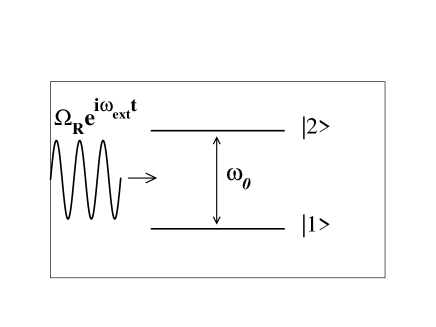
Figure 1: Josephson coupling of the two Zeeman levels $|1\rangle$ and $|2\rangle$ through an electromagnetic field with frequency $\omega_{\rm ext}$ and strength characterized by the Rabi frequency $\Omega_{R}$.

When the external potentials are the same ($V_{1}=V_{2}=V$) and the interactions strengths are equal ($g_{11}=g_{22}=g_{12}=g$), Eqs. (1)-(2) can be rewritten in a more compact form as:

$$i\frac{\partial{\psi}}{\partial t}=-\frac{1}{2}\Delta{\psi}+({\psi}^{\dagger}G\psi)\psi+V({\bf r})\psi+\alpha(t)P\psi,$$ (3)

where

$$\psi=\left(\begin{array}[]{c}\psi_{1}\\ \psi_{2}\end{array}\right),~{}~{}G=g\left(\begin{array}[]{cc}1&0\\ 0&1\end{array}\right),~{}~{}P=\left(\begin{array}[]{cc}0&1\\ 1&0\end{array}\right).$$ (4)

As a result of the fact that $G$ and $P$ commute, one can decompose the solution $\psi$ of the “inhomogeneous” problem described by Eq. (3) as

$$\psi(\vec{r},t)=U(t)\phi(\vec{r},t),$$ (5)

where $U(t)$ is the matrix of the homogeneous problem

$$U(t)=\exp{\left[-iP{\cal I}(t)\right]}=\left(\begin{array}[]{cc}\cos{{\cal I}(t)}&-i\sin{{\cal I}(t)}\\ -i\sin{{\cal I}(t)}&\cos{{\cal I}(t)}\end{array}\right),$$ (6)

with ${{\cal I}(t)}=\int_{0}^{t}\alpha(t^{\prime})dt^{\prime}$. Substituting Eq. (6) in Eq. (3), it is readily found that $\phi(\vec{r},t)$ satisfies the evolution equation decon

$$i\frac{\partial\phi}{\partial t}\equiv{\cal H}\phi=-\frac{1}{2}\Delta\phi+(\phi^{\dagger}G\phi)\phi+V(\vec{r})\phi,$$ (7)

which is identical to Eq. (3), but without the Rabi term proportional to $\alpha(t)P$.

When the external potentials or the interaction strengths are different, it is formally possible, as discussed in the Appendix A, to perform a decomposition like the one given in Eq. (5) and remove the Rabi term. However, this is done at the price of introducing time- and space- dependent effective interaction strengths in the nonlinear terms: in particular, for different external potentials the effective interaction strengths are both time- and space- dependent, while when the interaction strengths are different, a nonlinear Josephson term also arises in the nonlinear terms (i.e., $i\dot{\phi}_{1}$ is proportional to $\phi_{2}$ through terms proportional to products $\phi_{i}^{\ast}\phi_{j}$). As a result, the removal of the Rabi term is of little practical use and one has to resort to numerical or variational estimates: in the following, we will focus on the situation of different $g_{ij}$’s, and show that the efficiency of the Rabi switch for small deviations from the equal strengths situation can be effectively described by a two-mode model.

When the Rabi frequency is fixed, oscillations of atoms between the two components have been studied williams99 ; villain99 ; ohberg99 ; williams00 ; smerzi03 ; decon ; merhasin05 and experimentally observed williams00 ; smerzi03 . In the following, we consider a time-dependent Rabi frequency $\alpha(t)$: through a proper choice of a $\alpha(t)$, we can transfer the wavefunction of $|1\rangle$ to $|2\rangle$. More precisely, we propose a way to perform the following operation: at a time $t_{0}$, one has all the particles in $|1\rangle$ in the wavefunction $\psi_{1}(\vec{r},t_{0})$, and no particles in $|2\rangle$ ($\psi_{2}(\vec{r},t_{0})=0$). At a time $t_{1}$ we wish to have all the particles in $|2\rangle$ in the same wavefunction: $\psi_{2}(\vec{r},t_{1})=\psi_{1}(\vec{r},t_{0})$ (apart a phase factor). The protocol proposed in this paper allows the transfer of the wavefunction if $\psi_{1}(\vec{r},t_{0})$ is a stationary state (or a moving soliton, as discussed in Section IV) of the nonlinear Hamiltonian ${\cal H}$ defined in (7). If it is not, we can however have at the time $t_{1}$ all the particles in $|2\rangle$ in the wavefunction the condensate $|1\rangle$ would have had without the Rabi coupling [see Eq. (13)].

The proposed protocol works with or without nonlinearity: but with the nonlinearity on, one can transfer also a soliton wavefunction; for instance, in $1D$ one can have a matter-wave soliton of the species $|1\rangle$ propagating with velocity $v$, and after a time delay, the proposed Rabi switch will generate the same soliton with the same velocity in the species $|2\rangle$. Two remarks are due: (i) the transfer mechanism has the highest possible efficiency for equal interaction strengths, however it is very good and its efficiency is close to $1$ in a wider region in the relevant parameter space [in $1D$, deviations from the integrable case of equal interaction strengths are discussed through a two-mode ansatz]; (ii) the proposed mechanism is not copying the full many-body wavefunction of the weakly interacting Bose gas, but only the order parameter, which is related to the one-body density matrix.

To be more specific, we assume that $\alpha(t)$ depends on time as

$$\alpha(t)=\left\{\begin{array}[]{ll}0,&\hskip 28.45274pt0\leq t<t_{0},\\ \gamma,&\hskip 28.45274ptt_{0}\leq t\leq t_{1}=t_{0}+\delta,\\ 0,&\hskip 28.45274ptt>t_{1},\end{array}\right.$$ (8)

where $t_{0}$ is the switch-on time and $\delta$ denotes the duration of the Rabi pulse. From Eq. (8) we readily find

$${\cal I}(t)=\left\{\begin{array}[]{ll}0,&\hskip 28.45274pt0\leq t\leq t_{0},\\ \gamma(t-t_{0}),&\hskip 28.45274ptt_{0}\leq t\leq t_{1},\\ \gamma\delta,&\hskip 28.45274ptt\geq t_{1}.\end{array}\right.$$ (9)

Introducing the vector field $\phi$ by the decomposition in Eq. (6), it is observed that at the time $t_{0}$, i.e., before the switch-on of the Rabi pulse, $\psi(\vec{r},t_{0})=\phi(\vec{r},t_{0})$, while for $t_{0}\leq t\leq t_{1}$ we find that

$$\left\{\begin{array}[]{ll}\psi_{1}(\vec{r},t)=\cos{[\gamma(t-t_{0})]}\phi_{1}(\vec{r},t)-i\sin{[\gamma(t-t_{0})]}\phi_{2}(\vec{r},t),\\ \psi_{2}(\vec{r},t)=-i\sin{[\gamma(t-t_{0})]}\phi_{1}(\vec{r},t)+\cos{[\gamma(t-t_{0})]}\phi_{2}(\vec{r},t).\end{array}\right.$$ (10)

When the pulse duration is

$$\delta=\frac{\pi}{2\gamma},$$ (11)

at the end of the pulse we obtain

$$\left\{\begin{array}[]{ll}\psi_{1}(\vec{r},t_{1})=-i\phi_{2}(\vec{r},t_{1}),\\ \psi_{2}(\vec{r},t_{1})=-i\phi_{1}(\vec{r},t_{1}).\end{array}\right.$$ (12)

Since, in the interval $[t_{0},t_{1}]$, $\phi$ satisfies the homogeneous coupled GP equations (7), i.e. the same equations satisfied by the vector field $\psi$ in the interval $[0,t_{0}]$, then

$$\left(\begin{array}[]{c}\psi_{2}(\vec{r},t_{1})\\ \psi_{1}(\vec{r},t_{1})\end{array}\right)=-ie^{-i{\cal H}(t_{1}-t_{0})}\left(\begin{array}[]{c}\psi_{1}(\vec{r},t_{0})\\ \psi_{2}(\vec{r},t_{0})\end{array}\right).$$ (13)

Notice that if, instead of Eq. (8), one allows for a different time dependence of $\alpha(t)$, the time $t_{1}$ at which Eq. (13) holds is given by the condition $\cos{{\cal I}(t_{1})}=0$. For instance, with $\alpha(t)=0$ for $t<t_{0}$ and $t>t_{0}+\delta$, and $\alpha(t)=f(t)$ for $t_{0}\leq t\leq t_{0}+\delta$, the pulse duration $\delta$ such that Eq. (13) is valid is given by $\int_{0}^{\delta}dt^{\prime}f(t^{\prime}-t_{0})=\pi/2$.

We are interested in the situation in which no particles are in $|2\rangle$ at $t_{0}$ ($\psi_{2}(\vec{r},t_{0})$=0); this situation may occur, e.g., in the case where only a single condensate has been prepared (if, eventually, particles exist in the other component, it is possible to remove them by the suitable application of a Rabi pulse). Notice that this has been experimentally realized e.g. in the experiments of mertes07 (see also references therein). In such a case, Eq. (13) implies that at the end of the pulse one has that (apart from a phase factor) the wavefunction describing the condensate $|2\rangle$ is the same wavefunction which the condensate $|1\rangle$ would have had in $t_{1}$ in the absence of the Rabi pulse. We can quantify the success of the described protocol in several ways: one of them will be to define the “efficiency” $T$ as the fraction of atoms we are able to transfer from $|1\rangle$ to $|2\rangle$, i.e.,

$$T=\frac{N_{2}(t_{1})}{N_{1}(t_{0})},$$ (14)

where $N_{i}(t)=\int d\vec{r}|\psi_{i}\left(\vec{r},t\right)|^{2}$ is the number of particles in the condensate $i$ at time $t$. Notice that such a definition can even be extended in cases where the number of atoms in the second component is not zero initially by replacing in the numerator of Eq. (14) $N_{2}(t_{1})\rightarrow(N_{2}(t_{1})-N_{2}(t_{0}))$. Another more stringent way is to define a kind of “fidelity” $F$ of the wavefunction transfer, i.e., the quantity

$$F=\int d\vec{r}\,|\psi_{2}^{\ast}(\vec{r},t_{1})|\cdot|\psi_{1}(\vec{r},t_{0})|.$$ (15)

From Eq. (13) we see that the efficiency of Rabi switch is $1$ for equal interaction strengths, but the fidelity is not. However, we can have the fidelity to be equal to $1$ if $\psi$ is a stationary state of ${\cal H}$ corresponding to the eigenvalue $\mu$, i.e.

$${\cal H}\psi_{\mu}(\vec{r})=\mu\psi_{\mu}(\vec{r}).$$ (16)

If at time $t=0$, $\psi(\vec{r},0)=\psi_{\mu}(\vec{r})$, then $\phi(\vec{r},t_{0})=e^{-i\mu t_{0}}\psi_{\mu}(\vec{r})$ and

$$\left\{\begin{array}[]{ll}\psi_{1}(\vec{r},t_{1})=e^{-i\mu\delta}\left[\cos{(\gamma\delta)}\,\psi_{1}(\vec{r},t_{0})-i\sin{(\gamma\delta)}\,\psi_{2}(\vec{r},t_{0})\right],\\ \psi_{2}(\vec{r},t_{1})=e^{-i\mu\delta}\left[-i\sin{(\gamma\delta)}\,\psi_{1}(\vec{r},t_{0})+\cos{(\gamma\delta)}\,\psi_{2}(\vec{r},t_{0})\right].\end{array}\right.$$ (17)

When no particles are in $|2\rangle$ at $t_{0}$ and the pulse duration is given by Eq. (11), one has

$$\left\{\begin{array}[]{ll}\psi_{1}(\vec{r},t_{1})=0,\\ \psi_{2}(\vec{r},t_{1})=-ie^{-i\mu\delta}\psi_{1}(\vec{r},t_{0}).\end{array}\right.$$ (18)

Equations (18) show that the wavefunctions of the two components have been exchanged up to a phase factor. This remarkable feature allows us, again with equal interaction strengths $g_{ij}$, to transfer the condensate wavefunction (with $100\%$ efficiency) from a populated hyperfine state to an empty one. In the following section we discuss how to transfer from a condensate to the other the wavefunction of a moving matter-wave soliton.

We should further note about the latter that the nature of linear operators in the right hand-side of Eq. (3) is irrelevant in the derivation of Eq. (5). Hence, our analysis can be used to deal with:

• repulsively interacting as well as attractively interacting systems;

• continuum, as well as discrete systems;

• homogeneous systems (in the absence of external potentials) or inhomogeneous systems (e.g., in the presence of external harmonic trap and/or optical lattice potentials);

• one-dimensional systems or higher-dimensional ones.

In what follows, we illustrate the versatility of the Rabi switch by examining characteristic examples for each of the above settings. We will then illustrate, how the perfect efficiency of the matter wave transfer (discussed above for equal inter-particle interactions) is “degraded” in more realistic situations (where such interactions are no longer equal).

III Generalization to Multicomponent Bose-Einstein Condensates

The protocol discussed in the previous Section can be generalized for ${\cal N}\geq 2$ components with a suitable choice of the time dependence of the Rabi frequencies $\alpha_{ij}$ transferring particles from the condensate $i$ to the condensate $j$. For instance, for ${\cal N}=3$ and for equal potentials ($V_{1}=V_{2}=V_{3}\equiv V$) and interaction strengths ($g_{ij}\equiv g$), the relevant system of the three coupled GP equations can be written in the form of Eq. (3), namely

$$i\frac{\partial{\psi}}{\partial t}=-\frac{1}{2}\Delta{\psi}+({\psi}^{\dagger}G\psi)\psi+V({\bf r})\psi+\tilde{P}(t)\psi$$ (19)

with

$$\psi=\left(\begin{array}[]{c}\psi_{1}\\ \psi_{2}\\ \psi_{3}\end{array}\right),~{}~{}G=g\left(\begin{array}[]{ccc}1&0&0\\ 0&1&0\\ 0&0&1\end{array}\right),~{}~{}\tilde{P}=\left(\begin{array}[]{ccc}0&\alpha_{12}(t)&\alpha_{13}(t)\\ \alpha_{12}(t)&0&\alpha_{23}(t)\\ \alpha_{13}(t)&\alpha_{23}(t)&0\end{array}\right).$$ (20)

For general $\alpha_{ij}$, the decomposition $\psi=U\phi$ with

$$U=e^{-i\int_{0}^{t}\tilde{P}(t^{\prime})dt^{\prime}}$$ (21)

fails to recast Eq. (19) in the homogeneous form footnote ; however, it still removes the Rabi term when $\alpha_{ij}(t)=\alpha(t)$ for any $i,j$. With $\psi=U\phi$ and $U$ given by Eq. (21), one finds $i\frac{\partial{\phi}}{\partial t}=-\frac{1}{2}\Delta{\phi}+({\phi}^{\dagger}G\phi)\phi$. The matrix $U_{ij}(t)$ ($i,j=1,2,3$) has diagonal elements $U_{jj}=(1/3)\left[2\exp\left(i{\cal I}\right)+\exp\left(-2i{\cal I}\right)\right]$ and off-diagonal ones $U_{ij}=U_{jj}-\exp\left(i{\cal I}\right)$. Once the Rabi term has been removed, the “Rabi switch” described in the previous Section can be applied also for general ${\cal N}$ to transfer a wavefunction from a condensate to any one of the others.

Another choice of $\alpha_{ij}$ allowing for the removal of the Rabi term is provided by the generalization of Eq. (8), namely

$$\alpha_{ij}(t)=\left\{\begin{array}[]{ll}0,&\hskip 28.45274pt0\leq t\leq t_{0},\\ \gamma_{ij},&\hskip 28.45274ptt_{0}\leq t\leq t_{1},\\ 0,&\hskip 28.45274ptt\geq t_{1},\end{array}\right.$$ (22)

with all the $\alpha_{ij}$ turned on/off at the same time, but with eventually different intensities. As an example, for ${\cal N}=3$, one may consider $\gamma_{12}=a_{1}$, $\gamma_{13}=a_{2}$ and $\gamma_{23}=0$: the matrix $U(t)$, for $t_{0}\leq t\leq t_{1}$, then reads

$$U(t)=\left(\begin{array}[]{ccc}r_{1}(1+r_{2})&a_{1}r_{1}\frac{1-r_{2}}{\sqrt{a_{1}^{2}+a_{2}^{2}}}&a_{2}r_{1}\frac{1-r_{2}}{\sqrt{a_{1}^{2}+a_{2}^{2}}}\\ a_{1}r_{1}\frac{1-r_{2}}{\sqrt{a_{1}^{2}+a_{2}^{2}}}&\frac{a_{2}^{2}+a_{1}^{2}r_{1}(1+r_{2})}{a_{1}^{2}+a_{2}^{2}}&a_{1}a_{2}r_{1}\frac{(r_{3}-1)^{2}}{a_{1}^{2}+a_{2}^{2}}\\ a_{2}r_{1}\frac{1-r_{2}}{\sqrt{a_{1}^{2}+a_{2}^{2}}}&a_{1}a_{2}r_{1}\frac{(r_{3}-1)^{2}}{a_{1}^{2}+a_{2}^{2}}&\frac{a_{1}^{2}+a_{2}^{2}r_{1}(1+r_{2})}{a_{1}^{2}+a_{2}^{2}}\end{array}\right),$$ (23)

where

$$2r_{1}=r_{2}^{-1/2}=r_{3}^{-1}=\exp\left(-i\sqrt{a_{1}^{2}+a_{2}^{2}}\left(t-t_{0}\right)\right).$$ (24)

This allows us to determine the transfer of matter from the first to the second and third component. Similar results may be obtained in the more general case of ${\cal N}\geq 2$ components, i.e., “desirable” amounts of matter can be controllably directed to different hyperfine states according to their Rabi couplings. This general “Rabi router” is quite interesting in its own right, and it could be experimentally implemented in $F=1$ spinor condensates stamper ; chang04 ; higbie05 .

IV Results for $1$D settings

We now consider the $1$D version of Eqs. (1)-(2), which is relevant to the analysis of “cigar-shaped” condensates confined in highly anisotropic traps books ; reviews , and in dimensionless units reads

$$i\frac{\partial\psi_{1}}{\partial t}=\left[-\frac{1}{2}\frac{\partial^{2}}{\partial x^{2}}+V_{1}(x)+g_{11}|\psi_{1}|^{2}+g_{12}|\psi_{2}|^{2}\right]\psi_{1}+\alpha(t)\psi_{2},$$ (25)

$$i\frac{\partial\psi_{2}}{\partial t}=\left[-\frac{1}{2}\frac{\partial^{2}}{\partial x^{2}}+V_{2}(x)+g_{12}|\psi_{1}|^{2}+g_{22}|\psi_{2}|^{2}\right]\psi_{2}+\alpha(t)\psi_{1}.$$ (26)

We use wavefunctions $\psi_{i}(x,t)$ normalized to unity, so that $N_{1}(t)+N_{2}(t)=1$, with $N_{i}(t)=\int dx|\psi_{i}(x,t)|^{2}$. When the effect of the external potentials $V_{i}$ is negligible (as, e.g., in the case of potentials varying slowly on the soliton scale) and in absence of the Rabi coupling ($\alpha=0$), the system (25)-(26) becomes the Manakov system manakov , which is integrable for $g_{11}=g_{12}=g_{22}$. In what follows we examine both attractive and repulsive interatomic interactions, corresponding, respectively, to negative and positive values of the scattering lengths, and we will consider the effect of the presence of the trapping potential on the wavefunction transfer.

IV.1 Stationary bright matter-wave solitons

We consider in this subsection attractive interactions, $g_{ij}<0$, in absence of external potentials. Putting $\ell_{ij}=-g_{ij}$, we first consider the ideal case where $\ell_{11}=\ell_{12}=\ell_{22}\equiv\ell$ and assume that, at $t=0$, all the particles of $|1\rangle$ are described by the $1$-soliton solution of the nonlinear Schrödinger equation; thus, $\psi_{2}(x,0)=0$ and

$$\psi_{1}(x,0)=\frac{\sqrt{\ell}/2}{\cosh{(\ell x/2)}}.$$ (27)

In these units the soliton’s chemical potential is $\mu=-\ell^{2}/8$; turning on the Rabi coupling $\gamma$ at time $t_{0}$, and then turning it off at $t_{1}=t_{0}+\delta$, one gets, for $t_{0}\leq t\leq t_{1}$,

$$\psi(x,t)=\frac{\sqrt{\ell}/2}{\cosh{(\ell x/2)}}e^{-i\mu(t-t_{0})}\left(\begin{array}[]{c}\cos{\gamma(t-t_{0})}\\ -i\sin{\gamma(t-t_{0})}.\end{array}\right)$$ (28)

For $\delta=\pi/(2\gamma)$ no particles are in the condensate $|1\rangle$ at $t_{1}$, and the soliton wavefunction has been transferred in $|2\rangle$, i.e., $\psi_{2}(x,t_{1})=-(i/2)e^{-i\mu\delta}\sqrt{\ell}/\cosh{(\ell x/2)}$. The transfer of the soliton wavefunction is illustrated in Fig. 2(a)-(c).

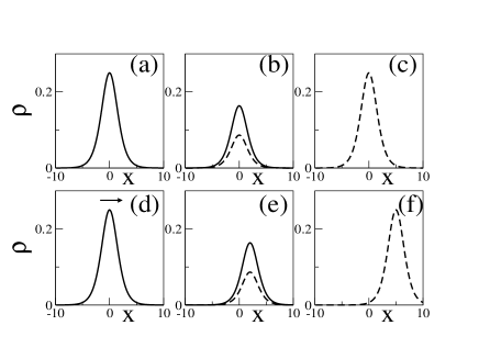
Figure 2: Transferring a stationary bright matter-wave soliton: in (a)-(b)-(c) the density $\rho_{j}=|\psi_{j}|^{2}$ is plotted for both components ($|1\rangle$ solid line; $|2\rangle$ dashed line) at the times $t=t_{0},t_{0}+0.4\delta,t_{1}$. In (d)-(e)-(f) the density is plotted at the same times, but for a velocity $v=1$ ($\delta=\pi/2$, $t_{1}=5$).

Notice that if we choose as initial condition

$$\left(\begin{array}[]{c}\psi_{1}(x,0)\\ \psi_{2}(x,0)\end{array}\right)=\frac{\sqrt{\ell}/2}{\cosh{(\ell x/2)}}\left(\begin{array}[]{c}\sqrt{N_{1}(0)}e^{i\varphi_{1}(0)}\\ \sqrt{N_{2}(0)}e^{i\varphi_{2}(0)}\end{array}\right),$$ (29)

i.e., two bright solitons with particle numbers $N_{1}(0)$, $N_{2}(0)$ and phase difference $\Delta\varphi(0)=\varphi_{2}(0)-\varphi_{1}(0)$, then, at $t=t_{1}$, we obtain

$$N_{1}(t_{1})=\left(\cos{(\gamma\delta)}\sqrt{N_{1}(0)}+\sin{(\gamma\delta)}\sin{\Delta\varphi(0)}\sqrt{N_{2}(0)}\right)^{2}+N_{2}(0)\sin^{2}{(\gamma\delta)}\cos^{2}{\Delta\varphi(0)}.$$ (30)

This shows that, by choosing properly the pulse duration and the initial phase difference, one can transfer a “desired” part of the soliton wavefunction from one condensate to the other.

Let us discuss now the interesting situation of different interaction strengths:the aim there is to study the efficiency of the Rabi switch of the soliton wavefunction and qualitatively understand the effect of the deviation from the ideal case. To that effect, we introduce a variational two-mode ansatz and confine ourselves to the situation in which no particles are initially in $|2\rangle$. For $t_{0}\leq t\leq t_{1}$, we choose the variational vectorial wavefunction

$$\psi_{V}=\left(\begin{array}[]{c}\psi_{v1}(x,t)\\ \psi_{v2}(x,t)\end{array}\right)=e^{-i\mu t}\left(\begin{array}[]{c}\sqrt{N_{1}(t)}e^{i\varphi_{1}(t)}\Phi_{1}(x)\\ \sqrt{N_{2}(t)}e^{i\varphi_{2}(t)}\Phi_{2}(x)\end{array}\right),$$ (31)

where

$$\Phi_{i}(x)=\frac{\sqrt{\ell_{ii}}/2}{\cosh{(\ell_{ii}x/2)}}.$$ (32)

The variational parameters are the numbers of particles $N_{i}(t)$ and their phases $\varphi_{i}(t)$. The variational vector wavefunction (31) has been used in pare to study the wavepacket dynamics for two linearly coupled nonlinear Schrödinger equations with $\ell_{11}=\ell_{22}$ and $\ell_{12}=0$. For general $\ell_{ij}$’s, the Lagrangian ${\cal L}=\frac{i}{2}\langle\psi_{V}^{\dagger}\frac{\partial\psi_{V}}{\partial t}-\frac{\partial\psi_{V}^{\dagger}}{\partial t}\psi_{V}\rangle-\langle\psi_{V}^{{\dagger}}\tilde{\cal H}\psi_{V}\rangle$ [where $\tilde{\cal H}$ is given by Eq. (52) and $\langle\rangle$ denotes spatial integration], is computed in Appendix B, where we show that the variational equations of motion for $N_{1}-N_{2}$ and $\varphi_{2}-\varphi_{1}$ are the equations of a (non-rigid) pendulum. The mass $M$ of the pendulum depends on the $\ell_{ij}$’s according Eq. (58) and for $\ell_{11}=\ell_{12}=\ell_{22}$ the pendulum mass is zero, allowing for the transfer of all the particles from a species to the other. When $\ell_{11}\neq\ell_{22}$, a detuning term in the pendulum equations is present [see Eq. (59)]. In the following, we will focus for simplicity on the more illuminating case $\ell_{11}=\ell_{22}$, with a general $\ell_{12}$.

Introducing the variables

$$\eta=N_{1}-N_{2};\,\,\,\varphi=\varphi_{2}-\varphi_{1},$$ (33)

one gets the equations of motion

$$\left\{\begin{array}[]{ll}\dot{\eta}=2\gamma\sqrt{1-\eta^{2}}\sin{\varphi},\\ \dot{\varphi}=-2\gamma\frac{\eta}{\sqrt{1-\eta^{2}}}\cos{\varphi}+\ell_{11}\frac{\ell_{12}-\ell_{11}}{6}\eta,\end{array}\right.$$ (34)

with initial conditions $\eta(t_{0})=1$ (i.e., all the particles initially in $|1\rangle$) and $\varphi(t_{0})=0$. It is worth noticing that Eqs. (34) are the same equations governing the tunneling of weakly-coupled BECs in a double-well potential smerzi97 ; raghavan99 (the only difference being that $\gamma$ corresponds to $-K$, where $K>0$ is the tunneling rate, which gives the same results for $\varphi\to\varphi+\pi$). Equations (34) are formally identical to the equations for an electron in a polarizable medium, where a polaron is formed kenkre86 . Analytical solutions have been found for the discrete nonlinear Schrödinger equations describing the motion of the polaron between two sites of a dimer kenkre86 ; kenkre87 .

Eqs. (34) are the equations of a non-rigid pendulum smerzi97 ; raghavan99 , with the effective Hamiltonian being

$$H_{eff}=\frac{M}{2}\eta^{2}+2\gamma\sqrt{1-\eta^{2}}\cos{\varphi},$$ (35)

where the pendulum mass is given by

$$M=\ell_{11}\frac{\ell_{12}-\ell_{11}}{6}.$$ (36)

When $\ell_{11}=\ell_{12}$, then the mass in Eq. (36) vanishes and $\ddot{\eta}=-4\gamma^{2}\eta$. The duration $\delta$ of the pulse needed to have a perfect switch is such that $\eta(t_{1}=t_{0}+\delta)=-1$, i.e. $\delta=\pi/(2\gamma)$ in agreement with Eq. (11). If the mass $M$ is positive (i.e., $g_{12}<g_{11}$), then it is still possible to transfer all the particles from $|1\rangle$ to $|2\rangle$, provided that the mass $M$ is smaller than a critical value $M_{c}$. If $M<M_{c}$, then the time $t_{1}$ at which $\eta(t_{1})=-1$ will be different from $t_{0}+\pi/(2\gamma)$ (the analytical computation of the tunneling period for a mass $M\neq 0$ is reported in the Appendix of raghavan99 ). This means that for deviations from the ideal case, one can optimize the transfer by choosing a pulse duration different from Eq. (11). This is illustrated in Fig. 3, where we compare $\eta(t)$ obtained from the two-mode equations (34) with the results of the numerical solution of the GP equations (25)-(26) for $\ell_{12}/\ell_{11}=13$: the numerical and variational results are in good agreement for a wide range of the parameters (see the inset of Fig. 3). The computation of $M_{c}$ is done according to the method discussed in smerzi97 : namely, one has to compute the point at which self-trapping occurs, and the result is

$$M_{c}=4\gamma.$$ (37)

For $\ell_{11}=1$, the critical value of $\ell_{12}$ is equal to $25$. A comparison with the numerical solution of the GP equations shows that this value is overestimated: e.g., at $M=3\gamma$, the efficiency $T$ at the optimal time is $\sim 0.9$, while it should be equal to $1$. However, the result (37) gives a reasonable estimate of the point at which is no longer possible to transfer with perfect efficiency all the particles from one condensate to the other, due to the self-trapping of the initial condensate wavefunction. Finally, we observe that, for $M<0$, the agreement between numerical and variational results is still good and the critical point is $M_{c}=-4\gamma$. We also notice that similar results can be obtained for the Rabi switch of $N$-soliton solutions.

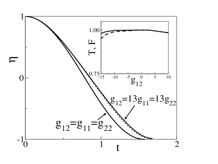
Figure 3: Comparison of the population imbalance $\eta(t)$ obtained from the numerical solution of the GP equations (25)-(26) [solid line] with the results of the two-mode equations (34) [dotted line] for $g_{12}=-1,-13$ given by Eq. (36) to a mass pendulum $M=0,2$, respectively. Inset: efficiency (solid line) and fidelity (dashed line), respectively defined according to Eqs. (14) and (15), and obtained from the numerical solution of the GP equations. Parameters used in both plots: $t_{0}=0$, $\gamma=1$, $g_{11}=g_{22}=-1$.

IV.2 Moving bright solitons and dark solitons

The proposed protocol works also for transferring moving solitons: with $\ell_{11}=\ell_{12}=\ell_{22}\equiv\ell$, one can prepare the initial wavefunction as

$$\psi(x,0)=\frac{\sqrt{\ell}/2}{\cosh{(\ell x/2)}}e^{ivx}\left(\begin{array}[]{c}\sqrt{N_{1}(0)}e^{i\varphi_{1}(0)}\\ \sqrt{N_{2}(0)}e^{i\varphi_{2}(0)}\end{array}\right).$$ (38)

For $t\leq t_{0}$ one has (with $\mu=-\ell^{2}/8$)

$$\psi(x,t)=\frac{\sqrt{\ell}/2}{\cosh{(\ell(x-vt)/2)}}e^{i(vx-\mu x-iv^{2}t/2)}\left(\begin{array}[]{c}\sqrt{N_{1}(0)}e^{i\varphi_{1}(0)}\\ \sqrt{N_{2}(0)}e^{i\varphi_{2}(0)}\end{array}\right),$$ (39)

so that at $t_{1}$, i.e., at the end of the pulse, $\delta=\pi/(2\gamma)$, one has

$$\psi(x,t_{1})=-i\frac{\sqrt{\ell}/2}{\cosh{(\ell(x-vt_{1})/2)}}e^{i(vx-\mu x-iv^{2}t_{1}/2)}\left(\begin{array}[]{c}\sqrt{N_{2}(0)}e^{i\varphi_{2}(0)}\\ \sqrt{N_{1}(0)}e^{i\varphi_{1}(0)}\end{array}\right).$$ (40)

If no particles are initially in $|2\rangle$, then one can transfer the moving soliton from a condensate to the other, as depicted in Fig. 2(d)-(f).

When the $\ell_{ij}$’s are different, one can use the same variational method discussed in the previous subsection. One needs to consider the variational wavefunction (31), but with a time-dependence included in the functions $\Phi$, which now read $\Phi_{i}(x,t)=(1/2)e^{ivx-iv^{2}t/2}\sqrt{\ell_{ii}}/\cosh{[\ell_{ii}(x-vt)/2]}$: apart form constant terms, we obtain the same Lagrangian [c.f. Eq. (53)] and the analysis is the same as before. In particular, the threshold for the self-trapping transition is still given by Eq. (37).

On the other hand, when the parameters $g_{ij}$ are positive and equal (and $V_{i}=0$), the soliton solution is now a dark matter-wave soliton, and one can transfer it from one condensate to the other. To examine the situation when the $g_{ij}$ are different and estimate the self-trapping threshold, one can also use a variational approach. Omitting the details, when $g_{11}=g_{22}$ one gets $M_{c}=4\gamma$, with $M=g_{11}(g_{12}-g_{11})n$, where $n$ is the (asymptotic) density of the dark soliton for very large $x$.

IV.3 Effect of the trapping potential

First, we consider repulsive condensates, in the ideal situation where $g_{11}=g_{12}=g_{22}=1$. An example of the realization of the Rabi switch for the ground state of the system is shown in the top panels of Fig. 4: we have considered an harmonic trapping potential of the form $V(x)=(1/2)\Omega^{2}x^{2}$. In the numerical simulations of the GP equations, we use $\Omega=0.08$, $t_{0}=10$ and $\gamma=\pi/10$; hence, after $t\geq 15$, the condensate wavefunctions have completely switched between components. Next, we consider the attractive case with $g_{11}=g_{12}=g_{22}=-1$. In this case, as an initial condition (for the first component) we have used a bright matter-wave soliton with the well-known sech-profile given by Eq. (27). As shown in the middle panels of Fig. 4, the transfer of the wavefunction is complete, just as in the repulsive case.

(a)	(b)
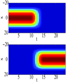
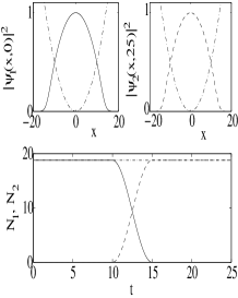
(c)	(d)
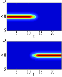
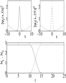
(e)	(f)

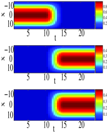
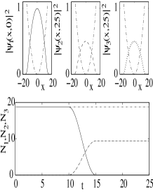
Figure 4: Panel (a) shows a space-time plot of the density $|\psi_{1}(x,t)|^{2}$ for the first component (top panel) and $|\psi_{2}(x,t)|^{2}$ for the second component (bottom panel). Panel (b) shows the spatial profile of $|\psi_{1}(x,t=0)|^{2}$ and $|\psi_{2}(x,t=25)|^{2}$ in solid and dashed lines respectively. The dash-dotted line shows the magnetic trap potential. They also show the evolution of the particle number $N_{i}=\int|\psi_{i}|^{2}dx$ for each of the components in the interval of the dynamical evolution. These features are shown in panels (a) and (b) for $g_{11}=g_{12}=g_{22}=1$. In panels (c) and (d), they are shown for a soliton in the case of $g_{11}=g_{12}=g_{22}=-1$. Analogous features are shown for $3$-component condensates in panels (e) and (f) (the third component is shown by dotted line in the right panel), again for the case with $g_{ij}=1$ for all $i,j=1,2,3$.

To better illustrate the versatility of the Rabi switch, even for ${\cal N}>2$, in Fig. 4 we have also considered the case with ${\cal N}=3$. In accordance with the results of the analysis carried in Section III, we use $a_{1}=a_{2}=(\pi/10)/\sqrt{2}$ between $t_{0}=10$ and $t=15$. In line with Eq. (23), at the end of this time interval, $r_{2}=-1$ and, as a result (due to the symmetry in the choice of $a_{1}$ and $a_{2}$), half of the matter initially at the first component is transferred to the second component and half to the third component, in excellent agreement with the results shown in the bottom panel of Fig. 4.

When the $g_{ij}$’s are different, the transfer will no longer be complete. As a measure of the deviation from the “ideal switch”, we characterize the degradation of the switch in this inhomogeneous case according to the relevant quantities introduced in Eq. (14) and (15). For repulsive condensates, we have considered the case of the ground state of ⁸⁷Rb, where the two spin states mentioned above have corresponding scattering lengths such that $g_{11}:g_{22}=0.97:1.03$. In this context, we have identified the ground state configuration for the first component alone and have subsequently applied the linear coupling for $\gamma=\pi/10$, for various values of $g_{12}$. The resulting transfer efficiency as a function of $g_{12}$ is shown in Fig. 5 (bottom right panel). The numerical result indicates that in the defocusing regime of repulsive inter-species interactions, the transfer efficiency and fidelity remain very high ($>0.9$) throughout the interval $-10<g_{12}<10$. Similar results have been obtained for attractive interactions $g_{11}=g_{22}=-1$ and varying $g_{22}$, starting form the ground state of the first component in presence of the trap.

(a)	(b)
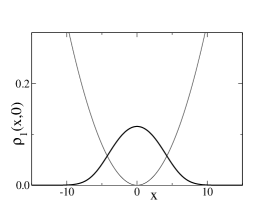
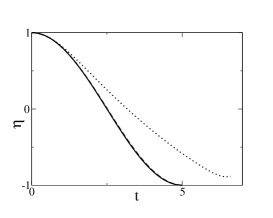
(c)	(d)
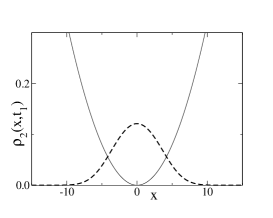
(e)	(f)

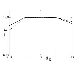
Figure 5: Panel (a) shows the initial condition: all the particles are in the ground state of the first component. The solid line shows the harmonic trapping potential. The parameters used in the GP equations are $\Omega=0.08$, $t_{0}=0$, $\gamma=\pi/10$, $g_{11}=0.97$, $g_{12}=1.03$. In (b) we plot the population imbalance $\eta(t)$ for $g_{12}=1$ (solid line), $-1$ (dashed line) and $-10$ (dotted line). The optimal times with the maximum transfer are respectively $t_{1}=5,5.02,6.48$. In (c), (d) and (e) we show the spatial profile $\rho_{2}(x,t_{1})\equiv|\psi_{2}(x,t_{1})|^{2}$ at these optimal times. In (e), where the transfer is not optimal, we plot also the the spatial profile $\rho_{1}(x,t_{1})\equiv|\psi_{1}(x,t_{1})|^{2}$. In panel (f) we show the transfer efficiency function $T$ (solid line) and the fidelity $F$ (dashed line) vs. the value of the inter-species interaction coefficient $g_{12}$.

We also performed similar computations in the case of attractive intra- and inter- species interactions for the solitonic initial condition (27) in the first component, which, with the trap confinement, is no longer the ground state. We have set the intra-species interactions at $g_{11}=g_{22}=-1$, varying $g_{12}$. Our findings are plotted in Fig. 6, showing the robustness of our protocol in a range of values of $g_{12}$ between $-3$ and $3$, a range smaller with respect to the case in which the initial condition is the ground state of the first component. This is due to the fact that the initial condition is not the ground state, and to the fact that the Rabi pulse used is homogeneous in space; note that (according to the analysis of Appendix A) a sort of space-dependent Rabi pulse would be needed to improve further the transfer efficiency. Finally, as expected, the Rabi switch is less effective in the case in which $g_{11}$ and $g_{22}$ have opposite signs. The qualitative reason is that the wavefunction, being a bright soliton which is supported by a negative coupling constant, cannot easily be transferred to an environment characterized by a positive coupling constant (which does not support bright solitons but rather dark ones). The fidelity and the efficiency are plotted in the panel (f) of Fig. 6.

(a)	(b)
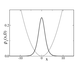
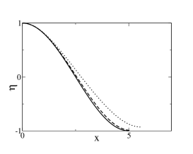
(c)	(d)
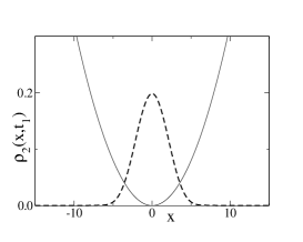
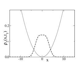
(e)	(f)

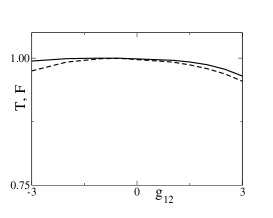
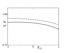
Figure 6: Panel (a) shows the initial condition: all the particles are in the soliton (27) of the first component. The parameters used are $\Omega=0.08$, $t_{0}=0$, $\gamma=\pi/10$, $g_{11}=g_{12}=-1$. In (b) we plot the population imbalance $\eta(t)$ for $g_{12}=-1$ (solid line), $1$ (dashed line) and $3$ (dotted line). The optimal times for maximum transfer are respectively $t_{1}=5,5.10,5.58$. In (c) and (d) we show the spatial profile of $\rho_{2}(x,t_{1})\equiv|\psi_{2}(x,t_{1})|^{2}$ at these optimal times for $g_{12}=1$ and $g_{12}=3$. In panel (e) we show the transfer efficiency function $T$ (solid line) and the fidelity $F$ (dashed line) vs. the value of the inter-species interaction coefficient $g_{12}$, and in (f) we plot the same quantities for $g_{11}=-1$, $g_{22}=1$ and the same initial condition: the efficiency is reduced with respect to the case $g_{11}=g_{22}=-1$.

V Results for $2D$ settings

Let us now consider the $2D$ version of Eqs. (1)-(2), pertaining to “pancake”-shaped condensates reviews . We will focus on the realistic case of a binary mixture of two hyperfine states of ⁸⁷Rb, with $g_{11}:g_{12}:g_{22}=0.97:1:1.03$, and examine both ground and excited states; the latter, will be characterized by the presence of one vortex or of many vortices arranged as vortex-lattice configurations. We shall consider only repulsive intra-species interactions, since for attractive ones, the system is generally subject to collapse reviews . In order to compare the results with the ones pertaining to the $1D$ setting, we vary the inter-species strength $g_{12}$ in the same domain (although for $g_{12}<0$ the system is also subject to collapse). In a real experiment this may be done by using external magnetic fields, which can change the magnitude and sign of the scattering length through the Feshbach resonance mechanism books .

It is relevant to consider at first the efficiency $T$ as a function of $g_{12}$, for different values of $\gamma$. The result is shown in the top panel of Fig. 7. In the 2D case, the transfer is almost complete as $T\geq 0.95$ for all positive values of $g_{12}<2$ (for $\gamma=\pi/10$). It is also seen that the efficiency is higher for larger values of the magnitude (or inverse duration) of the linear coupling coefficient $\gamma$.

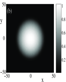
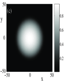
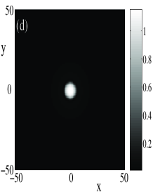
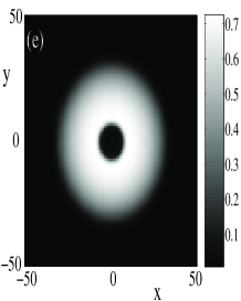
Figure 7: (a) The transmitivity function $T$ versus the inter-species strength $g_{12}$ for $\gamma=\pi/10$ (solid line) and $\gamma=\pi/20$ (dashed line). (b) Contour plot of the initial density of the ground state in the first component $\psi_{1}$. (c) Contour plot of the corresponding final density $|\psi_{2}(t=25)|^{2}$ of the second component for $g_{12}=1$; here the transfer of matter is complete. (d), (e) Contour plots of the corresponding final densities of both species, namely $|\psi_{1}(t=25)|^{2}$ and $|\psi_{2}(t=25)|^{2}$, but for $g_{12}=2$; as it is seen part of the matter remains (is missing) in the first (from the second) component.

We have considered the ground state of the system, shown in Fig. 7(b), in the first component $\psi_{1}$, for an harmonic trapping potential with strength $\Omega=0.045$ (the chemical potential is equal to one). In this case, assuming that the switch parameters are $t_{0}=10$ and $\gamma=\pi/10$, we have found the following: for $g_{12}=1$, the transfer of matter in the second component $\psi_{2}$ is complete [see Fig. 7(c) where the density of the second component at $t=25$ is shown], while for $g_{12}=2$ it is incomplete. In particular, as shown in Figs. 7(d)-(e) (where the densities $|\psi_{1}(t=25)|^{2}$ and $|\psi_{2}(t=25)|^{2}$ are respectively shown), a fraction of matter remains in the first component and is correspondingly missing from the central part of the second component after the switch-off of the Rabi pulse.

Next we consider an excited state, in which a vortex is initially placed at the center of the BEC cloud (first component). Here, it is interesting to investigate whether such a coherent nonlinear state can be transfered in the second component. As seen in Fig. 8(a), the efficiency is as high as for the ground state transfer. Also, for $g_{12}=1$, a perfect transfer of this excited state occurs as seen in Figs. 8(b) and (c), where the initial state of the first species and the final one of the second species are respectively shown. Nevertheless, for $g_{12}=2$, the transfer is not complete, as it can be seen in Figs. 8(d) and (e): starting again from the initial density shown in in Fig. 8(b), after the switch-off of the process, a ring-shaped part of the matter remains in (is missing from) the first (second) component. A careful observation of Fig. 8(d) also shows that this “high” density ring surrounds a low density ($\approx 0.2$) part of matter with a vortex on top of it. Note that even in this case, the vortex is transferred in the second component; on the other hand, the above mentioned “bright” and “dark” ring structures (respectively in the first and second component) do not carry any topological charge. It is interesting to remark that such methods are similar in spirit to the ones used to produce ring-like patterns in the recent experimental work of mertes07 .

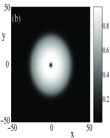
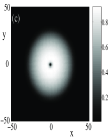
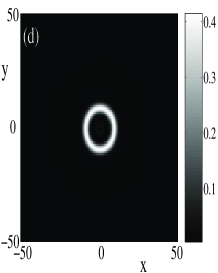
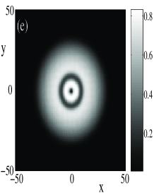
Figure 8: (a) Same as in Fig. 7(a). (b) The initial density of the first component $\psi_{1}$, consisting of a cloud with one vortex in the center. (c) The corresponding final density $|\psi_{2}(t=25)|^{2}$ of the second component for $g_{12}=1$; here the transfer is complete and the final configuration is identical to the initial one. (d), (e) The corresponding final densities of both species, namely $|\psi_{1}(t=25)|^{2}$ and $|\psi_{2}(t=25)|^{2}$, but for $g_{12}=2$.

Finally, we have considered a vortex cluster, namely a triangular vortex lattice, initially placed on top of the BEC of the first component. Similarly to what was found for the ground state and the single vortex, we find that the transfer efficiency function shown in Fig. 9(a) assumes values very close to $1$ for a wide range of values of $g_{12}$ (especially so in the case of short pulse durations i.e., fast transfer). As shown in the example of Figs. 9(b) and (c) for $g_{12}=1$ the vortex lattice in the first component is perfectly transferred to the second one. An “imperfect transfer”, for $g_{12}=2$, is shown in Figs. 9(d) and (e), corresponding to the final states of the first and second species when the initial state is as in Figs. 9(b). Here it is observed that small spots of matter (with densities $\approx 0.025$), each of which carries a vortex on it, remain in the first species, while a robust crystal structure is transferred to the second component. It is worth noting here that the vortex lattice remarkably appears to be even more robust, in its “switching properties”, than the ground state of the 2D system.

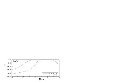
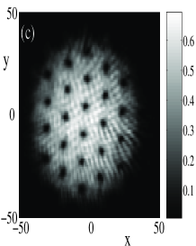
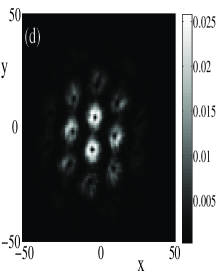
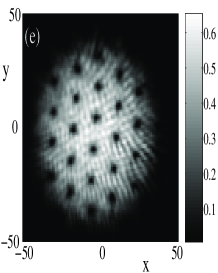
Figure 9: (a) Same as in Figs. 7(a) and 8(a). (b) The initial density of the first component $\psi_{1}$, consisting of a TF-cloud with a triangular vortex lattice ($\approx 24$ vortices). (c) The corresponding final density $|\psi_{2}(t=25)|^{2}$ of the second component for $g_{12}=1$; here the TF cloud and the vortex lattice are perfectly transferred to the second species. (d), (e) The corresponding final densities of both species, namely $|\psi_{1}(t=25)|^{2}$ and $|\psi_{2}(t=25)|^{2}$, but for $g_{12}=2$.

VI Conclusions and outlook

In this paper, we have systematically examined the possibility of using the linear Rabi coupling between the two (or more) components of a Bose-Einstein condensate as a means of controllably transferring the wavefunction of one condensate to the other. In particular, we have focused on the case of different hyperfine states, even though similar considerations are applicable to multicomponent condensates composed by different atomic species. We have illustrated that this transfer is exact and can be analytically studied in the limit where all inter- and intra- species interactions are equal. In addition, we have studied departures from this limit both numerically and by means of a two-mode ansatz, showing that in this two-mode description the impossibility to transfer all the particles from a condensate to the other is seen as the self-trapping of the initial condensate wavefunction. The threshold for the self-trapping has been compared in the homogeneous limit with the findings of the numerical simulations Gross-Pitaevskii equations.

The two-mode analysis shows that that for deviations from the ideal case one can optimize the transfer by choosing an appropriate pulse duration different from the duration given by Eq. (11) for equal interaction strengths . In the presence of external trapping potentials, our numerical simulations show that, for repulsive condensates (but, to a lesser extent, also for attractive condensates), the Rabi switch is very robust with high efficiency. In general, a change of sign of the inter-species interactions in $1$D has been shown to degrade –although, under appropriate conditions, not substantially– the efficiency of the transfer process. The switching was surprisingly found to be even more robust for particular types of coherent patterns, such as vortex lattices in pancake-shaped condensates. Furthermore, we have also illustrated that the generalization of the proposed Rabi switch to more than $2$ components can offer a possibility for systematically routing matter, in a controllable way, between different “atomic channels”.

It would be quite challenging to examine experimental realizations of such atomic switches and routers especially within the context of two hyperfine states, but also in that of spin-$1$ states recently studied in higbie05 ; sadler06 . Of particular interest in this setting would be the dynamics and phase separation of vortices and vortex lattices in multicomponent condensates. We expect that our mechanism may be relevant when transferring a condensate wavefunction also in different components of a dipolar BEC fattori07 .

Another relevant issue concerns the analysis of the role of the quantum fluctuations on the Rabi switch of wavefunctions: indeed, for two condensates (whose dynamics is described by coupled Gross-Pitaevskii equations) the Rabi switch is not copying the full many-body wavefunction of a component in the other, but only the (one-body) order parameter. Then, we expect that the presence of quantum fluctuations would naturally degrade the efficiency of our protocol. A study of such degradation is relevant for the implementation of a quantum register through a two-component Bose gas in an array of double-wells.

The protocol proposed in this paper allows the possibility to copy the wavefunction of a condensate into another species, providing a matter-wave counterpart for optical switches realized in nonlinear fiber optics agrawal . “All-optical switches” are very important tools in this context, allowing for to manipulate and eventually store the information contained in optical solitons. For this reason, the study of protocols focused on copying of wavefunctions in Bose condensates is deemed to be an important task towards an efficient manipulation of matter-wave solitons. Furthermore, one can think of a possible application of the present protocol to implement copies for quantum registers: indeed, one could perform some operations on a component (e.g., with a component in an array of double wells) and arrive at a desired wavefunction. At this point the wavefunction can be copied on the other component, and one can gain access (at a later time) to this information. In this respect, it would be very important to investigate the degradation of the quantum switch due to the quantum fluctuations.

Finally, since the protocol proposed in this paper is not restricted to linearly coupled Gross-Pitaevskii equations, one may safely expect that - once the effects of quantum corrections are accounted for - it can be extended to other sets of coupled equations such as the ones arising in the analysis of the weak pairing phase of $p$-wave superfluid states of cold atoms zoller and of quantum wires embedded in $p$-wave superconductors semenoff07 .

Acknoledgements Several stimulating discussions with E. Fersino, A. Michelangeli, and A. Smerzi are gratefully acknowledged. A.T. also thanks L. De Sarlo, F. Minardi and C. Fort of the Atomic Physics group at LENS for fruitful discussions. In the final stages of the project P.S. benefited from discussions with S. Flach, M. Gulacsi, M. Haque and S. Komineas. P.S. is grateful to the Particle Theory sector at S.I.S.S.A. for hospitality.

Appendix A Different potentials and interaction strengths

When the interaction strengths $g_{ij}$ are different (and, for simplicity, $V_{1}=V_{2}$), then Eqs. (1)-(2) can be written as

$$i\frac{\partial{\psi}}{\partial t}=-\frac{1}{2}\Delta{\psi}+V\psi+\sum_{j=1}^{2}({\psi}^{\dagger}G_{j}\psi)\sigma_{j}\psi+\alpha(t)P\psi,$$ (41)

with

$$G_{1}=\left(\begin{array}[]{cc}g_{11}&0\\ 0&g_{12}\end{array}\right),~{}~{}G_{2}=\left(\begin{array}[]{cc}g_{12}&0\\ 0&g_{22}\end{array}\right).$$ (42)

Upon removing the Rabi term in Eq. (41) by setting $\psi=U\phi$, with $U$ given by Eq. (6), one gets

$$i\frac{\partial{\phi}}{\partial t}=-\frac{1}{2}\Delta{\psi}+V\phi+\sum_{j=1}^{4}({\phi}^{\dagger}\tilde{G}_{j}\phi)\sigma_{j}\phi,$$ (43)

where $\tilde{G_{1}}={\cal L}_{1}-{\cal S}^{2}({\cal L}_{1}-{\cal L}_{2})$ and $\tilde{G_{2}}={\cal L}_{2}+{\cal S}^{2}({\cal L}_{1}-{\cal L}_{2})$, where the $2\times 2$ matrices ${\cal L}_{1,2}$ are defined by ${\cal L}_{1}=G_{1}-i{\cal S}\delta_{1}{\cal A}$ and ${\cal L}_{2}=G_{2}+i{\cal S}\delta_{2}{\cal A}$, with ${\cal A}=-i{\cal S}(\sigma_{1}-\sigma_{2})+{\cal C}(\sigma_{3}-\sigma_{4})$, ${\cal S}=\sin{{\cal I}(t)}$, ${\cal C}=\cos{{\cal I}(t)}$ and $\delta_{1}=g_{11}-g_{12}$, $\delta_{2}=g_{22}-g_{12}$. Furthermore $\tilde{G}_{3}=-i{\cal C}{\cal S}({\cal L}_{1}-{\cal L}_{2})=-\tilde{G}_{4}$. For $g_{11}=g_{12}=g_{22}=g$, then $\delta_{1}=\delta_{2}=0$ and $\tilde{G}_{1}=\tilde{G}_{2}=G$ and $G_{3}=G_{4}=0$, so that Eq. (7) is retrieved.

With different external potentials ($V_{1}(\vec{r})\neq V_{2}(\vec{r})$) and equal interaction strengths ($g_{11}=g_{22}=g_{12}=g$), Eqs. (1)-(2) can be written in a matrix form as

$$i\frac{\partial{\psi}}{\partial t}=\frac{1}{2}\left(-i\vec{\nabla}\right)^{2}{\psi}+\left({\psi}^{\dagger}G\psi\right)\psi+V_{1}({\bf r})\sigma_{1}\psi+V_{2}({\bf r})\sigma_{2}\psi+\alpha(t)P\psi,$$ (44)

where

$$\sigma_{1}=\left(\begin{array}[]{cc}1&0\\ 0&0\end{array}\right),~{}~{}\sigma_{2}=\left(\begin{array}[]{cc}0&0\\ 0&1\end{array}\right),~{}~{}\sigma_{3}=\left(\begin{array}[]{cc}0&1\\ 0&0\end{array}\right)~{}~{}\sigma_{4}=\left(\begin{array}[]{cc}0&0\\ 1&0\end{array}\right),$$ (45)

and $G$ given in Eq. (4). It is yet possible to perform a decomposition permitting to formally write Eq. (44) without the Rabi term $\alpha(t)P\psi$. We set $\psi=U\phi$, with

$$U=\left(\begin{array}[]{cc}u_{1}&u_{3}\\ u_{4}&u_{2}\end{array}\right):$$ (46)

the Rabi term vanishes, provided that the functions $u_{j}(\vec{r},t)$ ($j=1,\cdots,4$) obey the (linear) matrix equation

$$i\frac{\partial{U}}{\partial t}=-\frac{1}{2}\Delta{U}+\alpha(t)PU+{\cal V}(\vec{r})\left(u_{3}\sigma_{3}-u_{4}\sigma_{4}\right),$$ (47)

where ${\cal V}(\vec{r})=V_{1}(\vec{r})-V_{2}(\vec{r})$. This matrix equation corresponds to four equations for $u_{1}$, $u_{2}$, $u_{3}$, and $u_{4}$, which are grouped in two pairs, one for $u_{1}$ and $u_{4}$, namely

$$i\frac{\partial u_{1}}{\partial t} = -\frac{1}{2}\Delta u_{1}+\alpha(t)u_{4},$$ (48)

$$i\frac{\partial u_{4}}{\partial t} = -\frac{1}{2}\Delta u_{4}-{\cal V}(\vec{r})u_{4}+\alpha(t)u_{1},$$ (49)

and a similar for $u_{2}$ and $u_{3}$ (with ${\cal V}(\vec{r})$ instead of $-{\cal V}(\vec{r})$). Eqs. (48)-(49) are two coupled linear Schrödinger equations, and the difference between the potentials ${\cal V}$ enters as an effective potential in one of the two equations. When ${\cal V}=0$, the result $u_{1}=u_{2}=\cos{{\cal I}(t)}$ and $u_{3}=u_{4}=-i\sin{{\cal I}(t)}$ is readily obtained.

With the functions $u_{j}$ defined by Eq. (47), then $\phi$ satisfies the equation

$$i\frac{\partial{\phi}}{\partial t}=\frac{1}{2}\left(-i\vec{\nabla}\right)^{2}{\phi}+\left({\phi}^{\dagger}\tilde{G}\phi\right)\phi+V_{1}({\bf r})\sigma_{1}\phi+V_{2}({\bf r})\sigma_{2}\phi+\vec{{\cal X}}\cdot\vec{\nabla}\phi,$$ (50)

with $\tilde{G}=U^{\dagger}GU$ and $\vec{{\cal X}}=\vec{{\cal X}}(\vec{r},t)=-U^{-1}\vec{\nabla}U$. Eq. (50) can be written in the form

$$i\frac{\partial{\phi}}{\partial t}=\frac{1}{2}\left(-i\vec{\nabla}+i\vec{{\cal X}}\right)^{2}{\phi}+\left({\phi}^{\dagger}\tilde{G}\phi\right)\phi+V_{1}({\bf r})\sigma_{1}\phi+V_{2}({\bf r})\sigma_{2}\phi+{\cal Y}\phi,$$ (51)

where ${\cal Y}=\left(\vec{{\cal X}}^{2}-\vec{\nabla}\cdot\vec{{\cal X}}\right)/2$, showing that, with different external potentials, an effective complex vector potential acts on the multicomponent gas and the effective interaction strengths are both time- and space- dependent [since the $\tilde{G}$ depends upon the $U(\vec{r},t)$].

Appendix B Two-Mode Variational Equations

For the pulse (8) and at times $t_{0}\leq t\leq t_{0}+\delta$, the Lagrangian to be computed is given by ${\cal L}=\frac{i}{2}\langle\psi_{V}^{\dagger}\frac{\partial\psi_{V}}{\partial t}-\frac{\partial\psi_{V}^{\dagger}}{\partial t}\psi_{V}\rangle-\langle\psi_{V}^{{\dagger}}\tilde{\cal H}\psi_{V}\rangle$, where

$$\tilde{\cal H}=\left(\begin{array}[]{cc}K-\frac{\ell_{11}}{2}|\psi_{v1}|^{2}-\frac{\ell_{12}}{2}|\psi_{v2}|^{2}&\gamma\\ \gamma&K-\frac{\ell_{12}}{2}|\psi_{v1}|^{2}-\frac{\ell_{22}}{2}|\psi_{v2}|^{2}\end{array}\right),$$ (52)

$\psi_{V}$ is defined in Eq. (31) and $K=-\frac{1}{2}\frac{\partial^{2}}{\partial x^{2}}$. Then, one gets

$${\cal L}=-N_{1}\dot{\varphi}_{1}-N_{2}\dot{\varphi}_{2}-\gamma\sqrt{\frac{\ell_{22}}{\ell_{11}}}F\left(\frac{\ell_{22}}{\ell_{11}}\right)\sqrt{N_{1}N_{2}}\cos{(\varphi_{1}-\varphi_{2})}-\frac{\ell_{11}^{2}}{24}N_{1}-\frac{\ell_{22}^{2}}{24}N_{2}+\mu+$$

$$+\frac{\ell_{11}^{2}}{12}N_{1}^{2}+\frac{\ell_{22}^{2}}{12}N_{2}^{2}+\frac{\ell_{22}}{8}\ell_{12}L\left(\frac{\ell_{22}}{\ell_{11}}\right)N_{1}N_{2},$$ (53)

where the functions $F(\theta)$ and $L(\theta)$ are defined as

$$F(\theta)\equiv\int_{-\infty}^{\infty}\frac{dy}{\cosh{(y)}\cosh{(\theta y)}};\,\,\,L(\theta)\equiv\int_{-\infty}^{\infty}\frac{dy}{\cosh^{2}{(y)}\cosh^{2}{(\theta y)}}.$$ (54)

Note that $F(0)=\pi$, $F(1)=2$, $L(0)=2$, and $L(1)=4/3$, while both functions $\to 0$ as $\theta\to\infty$. For small values of $\delta\theta=\theta-1$, one has $F(\theta)\approx 2-\delta\theta+\frac{24-\pi^{2}}{36}\delta\theta^{2}$ and $L(\theta)\approx\frac{4}{3}-\frac{2}{3}\delta\theta-\frac{2(\pi^{2}-15)}{45}\delta\theta^{2}$. For $\ell_{11}=\ell_{22}$, from Eq. (53) one gets, apart from constant terms, the Lagrangian

$${\cal L}=-N_{1}\dot{\varphi}_{1}-N_{2}\dot{\varphi}_{2}-2\gamma\sqrt{N_{1}N_{2}}\cos{(\varphi_{1}-\varphi_{2})}+\frac{\ell_{11}^{2}}{12}N_{1}^{2}+\frac{\ell_{22}^{2}}{12}N_{2}^{2}+\frac{\ell_{11}\ell_{12}}{6}N_{1}N_{2}.$$ (55)

Introducing the variables (33), the equations of motions for $\eta$ and $\varphi$ obtained from the Lagrangian (53) are

$$\left\{\begin{array}[]{ll}\dot{\eta}=2\gamma^{\prime}\sqrt{1-\eta^{2}}\sin{\varphi},\\ \dot{\varphi}=-2\gamma^{\prime}\frac{\eta}{\sqrt{1-\eta^{2}}}\cos{\varphi}+\Delta E+M\eta,\end{array}\right.$$ (56)

where

$$\gamma^{\prime}=\frac{\gamma}{2}\sqrt{\frac{\ell_{22}}{\ell_{11}}}F\left(\frac{\ell_{22}}{\ell_{11}}\right),$$ (57)

$$M=\frac{1}{12}\left[\frac{3}{2}\ell_{12}\ell_{22}L\left(\frac{\ell_{22}}{\ell_{11}}\right)-\ell_{11}^{2}-\ell_{22}^{2}\right],$$ (58)

and

$$\Delta E=\frac{1}{24}\left(\ell_{22}^{2}-\ell_{11}^{2}\right).$$ (59)

The variables $\eta,\varphi$ are canonically conjugate dynamical ones with respect to the effective Hamiltonian

$$H_{eff}=\frac{M}{2}\eta^{2}+2\gamma^{\prime}\sqrt{1-\eta^{2}}\cos{\varphi}+\Delta E\cdot\eta.$$ (60)

Equation (60) is the Hamiltonian of a non-rigid pendulum, whose mass and length depend on the parameters $\ell_{ij}$. For $\ell_{11}=\ell_{22}$, then $M=\ell_{11}(\ell_{12}-\ell_{11})/6$, $\Delta E=0$ and $\gamma^{\prime}=\gamma$, retrieving Eq. (34) and the effective Hamiltonian (35). When $\ell_{12}=\ell_{11}=\ell_{22}$, then the mass of the pendulum is vanishing. When $\ell_{11}\neq\ell_{22}$, then the presence of the detuning $\Delta E$ favours self-trapping and can be studied as in raghavan99 .

References

- (1) C. J. Pethick and H. Smith, Bose-Einstein Condensation in Dilute Alkali Gases, Cambridge University Press (Cambridge, 2002); L. P. Pitaveskii and S. Stringari, Bose-Einstein Condensation, Clarendon Press (Oxford, 2003).
- (2) F. Dalfovo, S. Giorgini, L. P. Pitaveskii and S. Stringari, Rev. Mod. Phys. 71, 463 (1999); A. J. Leggett, Rev. Mod. Phys. 73, 307 (2001); P. G. Kevrekidis and D. J. Frantzeskakis, Mod. Phys. Lett. B 18, 173 (2004); V. A. Brazhnyi and V. V. Konotop, Mod. Phys. Lett. B 18, 627 (2004).
- (3) D. M. Stamper-Kurn, M. R. Andrews, A. P. Chikkatur, S. Inouye, H.-J. Miesner, J. Stenger, and W. Ketterle, Phys. Rev. Lett. 80, 2027 (1998).
- (4) A. E. Leanhardt, Y. Shin, D. Kielpinski, D. E. Pritchard, and W. Ketterle, Phys. Rev. Lett. 90, 140403 (2003).
- (5) R. Dumke, M. Johanning, E Gomez, J. D. Weinstein, K. M. Jones, and P. D. Lett, New. J. Phys. 8, 64 (2006).
- (6) C. J. Myatt, E. A. Burt, R. W. Ghrist, E. A. Cornell, and C. E. Wieman, Phys. Rev. Lett. 78, 586 (1997).
- (7) D. S. Hall, M. R. Matthews, J. R. Ensher, C. E. Wieman, and E. A. Cornell, Phys. Rev. Lett. 81, 1539 (1998).
- (8) J. Williams, R. Walser, J. Cooper, E. A. Cornell, and M. Holland, Phys. Rev. A 61, 033612 (2000).
- (9) P. Maddaloni, M. Modugno, C. Fort, F. Minardi, and M. Inguscio, Phys. Rev. Lett. 85, 2413 (2000).
- (10) A. Smerzi, A. Trombettoni, T. Lopez-Arias, C. Fort, P. Maddaloni, F. Minardi, and M. Inguscio, Eur. Phys. J. B 31, 457 (2003).
- (11) O. Mandel, M. Greiner, A. Widera, T. Rom, T. W. Hänsch, and I. Bloch, Phys. Rev. Lett. 91, 010407 (2003).
- (12) M.-S. Chang, C. D. Hamley, M. D. Barrett, J. A. Sauer, K. M. Fortier, W. Zhang, L. You, and M. S. Chapman, Phys. Rev. Lett. 92, 140403 (2004).
- (13) M. H. Wheeler, K. M. Mertes, J. D. Erwin, and D. S. Hall, Phys. Rev. Lett. 93, 170402 (2004).
- (14) V. Schweikhard, I. Coddington, P. Engels, S. Tung, and E. A. Cornell, Phys. Rev. Lett. 93, 210403 (2004).
- (15) J. M. Higbie, L. E. Sadler, S. Inouye, A. P. Chikkatur, S. R. Leslie, K. L. Moore, V. Savalli, and D. M. Stamper-Kurn, Phys. Rev. Lett. 95, 050401 (2005).
- (16) J. Kronjager, C. Becker, P. Navez, K. Bongs, and K. Sengstock, Phys. Rev. Lett. 97, 110404 (2006).
- (17) L. E. Sadler, J. M. Higbie, S. R. Leslie, M. Vengalattore, and D. M. Stamper-Kurn, Nature 443, 312 (2006).
- (18) N. Lundblad, R. J. Tompson, D. C. Aveline, and L. Maleki, Optics Express 14. 10164 (2006).
- (19) M. Vengalattore, J. M. Higbie, S. R. Leslie, J. Guzman, L. E. Sadler, and D. M. Stamper-Kurn, Phys. Rev. Lett. 98, 200801 (2007).
- (20) K. M. Mertes, J. W. Merrill, R. Carretero-González, D. J. Frantzeskakis, P. G. Kevrekidis, and D. S. Hall, Phys. Rev. Lett. 99, 190402 (2007).
- (21) G. Modugno, G. Ferrari, G. Roati, R.J. Brecha, A. Simoni, M. Inguscio, Science 294, 1320 (2001).
- (22) J. Catani, L. De Sarlo, G. Barontini, F. Minardi, and M. Inguscio, arXiv:0706.2781.
- (23) M. Mudrich, S. Kraft, K. Singer, R. Grimm, A. Mosk, and M. Weidemüller, Phys. Rev. Lett. 88, 253001 (2002).
- (24) T.-L. Ho and V.B. Shenoy, Phys. Rev. Lett. 77, 3276 (1996).
- (25) H. Pu and N.P. Bigelow, Phys. Rev. Lett. 80, 1130 (1998).
- (26) B.D. Esry, C.H. Greene, J.P. Burke, Jr, and J.L. Bohn, Phys. Rev. Lett. 78, 3594 (1997).
- (27) Th. Busch, J. I. Cirac, V. M. Perez-Garcia, and P. Zoller, Phys. Rev. A 56, 2978 (1997); R. Graham and D. Walls, Phys. Rev. A 57, 484 (1998); H. Pu and N. P. Bigelow, Phys. Rev. Lett. 80, 1134 (1998); B. D. Esry and C. H. Greene, Phys. Rev. A 57, 1265 (1998).
- (28) M. Trippenbach, K. Góral, K. Rzazewski, B. A. Malomed, and Y. B. Band, J. Phys. B 33, 4017 (2000); S. Coen and M. Haelterman, Phys. Rev. Lett. 87, 140401 (2001); B. A. Malomed, H. E. Nistazakis, D. J. Frantzeskakis, and P. G. Kevrekidis, Phys. Rev. A 70, 043616 (2004).
- (29) Th. Busch and J. R. Anglin, Phys. Rev. Lett. 87, 010401 (2001); P. Öhberg and L. Santos, Phys. Rev. Lett. 86, 2918 (2001); P. G. Kevrekidis, H. E. Nistazakis, D. J. Frantzeskakis, B. A. Malomed, and R. Carretero-González, Eur. Phys. J. D 28, 181 (2004).
- (30) B. Deconinck, P. G. Kevrekidis, H. E. Nistazakis, and D. J. Frantzeskakis, Phys. Rev. A 70, 063605 (2004).
- (31) M. A. Porter, P. G. Kevrekidis, and B. A. Malomed, Physica D 196, 106 (2004).
- (32) G.-H. Chen and Y.-S. Wu, Phys. Rev. A 67, 013606 (2003).
- (33) A. Kuklov, N. Prokofev, and B. Svistunov, Phys. Rev. Lett. 92, 030403 (2004).
- (34) G.-P. Zheng, J.-Q. Liang, and W. M. Liu, Phys. Rev. A 71, 053608 (2005).
- (35) R. V. Pai, K. Sheshadri, and R. Pandit, PhysṘev. B 77, 014503 (2008).
- (36) J. Stenger, S. Inouye, D. M. Stamper-Kurn, H.-J. Miesner, A. P. Chikkatur, and W. Ketterle, Nature (London) 396, 345 (1998).
- (37) J. Ieda, T. Miyakawa, and M. Wadati, Phys. Rev. Lett. 93, 194102 (2004); J. Phys. Soc. Jpn. 73, 2996 (2004); M. Wadati and N. Tsuchida, J. Phys. Soc. Jpn. 75, 014301 (2006).
- (38) L. Li, Z. Li, B. A. Malomed, D. Mihalache, and W. M. Liu, Phys. Rev. A 72, 033611 (2005); L. Salasnich and B. A. Malomed, Phys. Rev. A 74, 053610 (2006).
- (39) H. E. Nistazakis, D. J. Frantzeskakis, P. G. Kevrekidis, B. A. Malomed, R. Carretero-González, arXiv:0705.1324.
- (40) B. J. Dabrowska-Wüster, E. A. Ostrovskaya, T. J. Alexander, and Y. S. Kivshar, Phys. Rev. A 75, 023617 (2007).
- (41) H. Saito, and M. Ueda, Phys. Rev. A 72, 023610 (2005); K. Murata, H. Saito, and M. Ueda, Phys. Rev. A 75, 013607 (2007).
- (42) B. A. Malomed, Phys. Rev. A 43, 410 (1991); M. J. Potasek, J. Opt. Soc. Am. B 10, 941 (1993).
- (43) Y. S. Kivshar and G. P. Agrawal, Optical Solitons: from Fibers to Photonic Crystals, CA Academic Press (San Diego, 2003).
- (44) D. M. Stamper-Kurn and W. Ketterle, Spinor condensates and light scattering from Bose-Einstein condensates, in R. Kaiser, C. Westbrook, and F. David eds., Coherent Atomic Matter Waves, Les Houches Summer School Session LXXII, Springer (New York, 2001), pp. 137-217 (arXiv:cond-mat/0005001).
- (45) D. S. Hall, Multi-Component Condensates: Experiment, in P.G. Kevrekidis, D.J. Frantzeskakis, and R. Carretero-Gonzalez eds., Emergent Nonlinear Phenomena in Bose-Einstein Condensates, Springer Series on Atomic, Optical, and Plasma Physics, 2007, pp. 307-327.
- (46) A. Smerzi, S. Fantoni, S. Giovanazzi, and S. R. Shenoy, Phys. Rev. Lett. 79, 4950 (1997).
- (47) M. Albiez, R. Gati, J. Fölling, S. Hunsmann, M. Cristiani, and M. K. Oberthaler, Phys. Rev. Lett. 95, 010402 (2005).
- (48) J. I. Cirac, M. Lewenstein, K. Molmer, and P. Zoller, Phys. Rev. A 57, 1208 (1998).
- (49) P. Villain and M. Lewenstein, Phys. Rev. A 59, 2250 (1999).
- (50) Notice that one can pass from to simply by shifting the phase difference between the condensate wavefunctions (where ) of : .
- (51) J. Williams, R. Walser, J. Cooper, E. Cornell, and M. Holland, Phys. Rev. A 59, R31 (1999).
- (52) P. Öhberg and S. Stenholm, Phys. Rev. A 59, 3890 (1999).
- (53) I. M. Merhasin, B. A. Malomed, and R. Driben, J. Phys. B 38, 877 (2005); I. M. Merhasin, B. A. Malomed, and R. Driben, Phys. Scripta T116, 18 (2005).
- (54) Using the notation , with the time-dependent matrix defined by , we observe that when the matrices and commute, then the decomposition allows to cast Eq. (19) in the homogeneous form.
- (55) S. V. Manakov, Zh. Eksp. Teor. Fiz. 65, 505 (1973) [Sov. Phys. JETP 38, 248 (1974)].
- (56) C. Paré and M. Florjańczyk, Phys. Rev. A 41, 6287 (1990).
- (57) S. Raghavan, A. Smerzi, S. Fantoni, and S. R. Shenoy, Phys. Rev. A 59, 620 (1999).
- (58) V. M. Kenkre and D. K. Campbell, Phys. Rev. B 34, 4959 (1986).
- (59) V. M. Kenkre and G. P. Tsironis, Phys. Rev. B 35, 1473 (1987).
- (60) T. Lahaye, T. Koch, B. Froehlich, M. Fattori, J. Metz, A. Griesmaier, S. Giovanazzi, and T. Pfau, Nature 448, 672 (2007).
- (61) S. Tewari, S. Das Sarma, C. Nayak, C. Zhang, and P. Zoller, Phys. Rev. Lett. 98, 010506 (2007).
- (62) G. W. Semenoff and P. Sodano, J. Phys. B 40, 1479 (2007).