Domain-wall structure of a classical Heisenberg ferromagnet on a Möbius strip

Abstract

We study theoretically the structure of domain walls in ferromagnetic states on Möbius strips. A two-dimensional classical Heisenberg ferromagnet with single-site anisotropy is treated within a mean-field approximation by taking into account the boundary condition to realize the Möbius geometry. It is found that two types of domain walls can be formed, namely, parallel or perpendicular to the circumference, and that the relative stability of these domain walls is sensitive to the change in temperature and an applied magnetic field. The magnetization has a discontinuity as a function of temperature and the external field.

I Introduction

The effect of system geometry on the physical properties has stimulated renowned interest after the realization of crystals with unusual shapes, e.g., ring, cylinder and especially Möbius strip,Tanda1 ; Tanda2 ; Okajima ; Tanda because the ordered states in these systems could be quite different from those in the ordinary bulk systems. These single crystals are made of quasi-one-dimensional conductors, such as, NbSe₃.

Hayashi and EbisawaHayashi-Ebisawa studied the $s$-wave superconducting (SC) states on a Möbius strip based on the Ginzburg-Landau (GL) theory, and found that the Little-Parks oscillation is modified compared to that for the ordinary ring-shaped samples. When the flux quanta threading the Möbius strip are close to half-odd integer times flux quantum $\phi_{0}=hc/2e$ ($h$, $c$, and $-e$ being the Planck constant, the speed of light and the electron charge, respectively), a state appears in which the real-space node in SC gap exists along the circumference of the strip. Later a more detailed examination using the Bogoliubov-de Gennes (BdG) theory confirmed this prediction.HEK Charge density wave (CDW) states in ring-shaped crystals were also examined by Nogawa and Nemoto, Nogawa and Hayashi et al.HEKdis ; HEKcdw There the effect of frustration due to bending of the lattice was clarified. The persistent current in a Möbius strip as a function of the applied flux was examined by Yakubo et al.Yakubo and Mila et al.Mila Wakabayashi and HarigayaWakabayashi-Harigaya studied the Möbius strip made of a nanographite ribbon, and the effect of Möbius geometry on the edge localized states has been explored. Kaneda and Okabe Kaneda-Okabe studied the Ising model on Möbius, especially the effect of sample geometry on the finite scaling properties.

In this paper we study the ferromagnetic states on Möbius strips. Although the single crystals with Möbius geometry have been obtained for systems with CDW or superconducting order up to now, we expect that the synthesis of ferromagnetic Möbius strips using quasi-one-dimensional ferromagnets could be possible. In such a system there should be a domain wall (DW), and two kinds of DWs, i.e., those parallel and perpendicular to the circumference are expected. We will show that these two types of DWs can actually exist. An interesting point is that the relative stability of these two kinds of DWs is quite sensitive to the change in temperature and the applied magnetic field. We expect that this might be used in the field of technological applications in future.

This paper is organized as follows. In Sec. II the model and the method of calculations are presented. We study the structure of domain walls on Möbius strips in Sec. III. In Sec. IV the effect of an applied magnetic field is examined. Section V is devoted to summary.

II Model and Mean-field approximation

In order to study the ferromagnetic states on Möbius strips we consider a classical Heisenberg model with single-ion anisotropy, since this model is most suitable to examine the spatial variations of the magnetization.

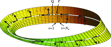
Figure 1: Schematic picture of a Möbius strip. The axes are those for the relative coordinate system at each point. See text for details.

A model system with Möbius geometry is constructed as follows. We consider $N_{y}$ (even integer) sets of ferromagnetic chains (each chain has $N_{x}$ sites; $N_{x}$ being an integer), and these chains are weakly coupled ferromagnetically. We denote the $i$ th spin on the $j$ th chain ($1\leq i\leq N_{x}$, $1\leq j\leq N_{y}$) as ${\bf S}_{i,j}$ ($|{\bf S}_{i,j}|=1$). As a first step we form a cylinder, where the circumference is parallel to the chains. If one moves one site along the chain, the direction normal to the strip changes by the angle $\theta_{1}\equiv 2\pi/N_{x}$. Then we twist the strip along the circumference at the middle of the strip (shown as a white curve in Fig.1) so that the twist angles at the neighboring sites on the white curve (for example, the points denoted as $P$ and $Q$) differ by $\theta_{2}\equiv\pi/N_{x}$. Finally the boundary condition is imposed,

$${\bf S}_{N_{x}+1,j}={\bf S}_{1,N_{y}+1-j},$$ (1)

to get a Möbius strip. The direction normal to the strip is different from site to site, so we define the absolute coordinate system $(x,y,z)$ and the relative coordinate system $({\tilde{x}},{\tilde{y}},{\tilde{z}})$ at each point and use one of them which is better to describe the particular situation. For the former, the point with $i=1$ on the middle of the strip ($P$ in Fig.1) is taken to be the origin, and the $z$ direction is perpendicular to the strip. The $x$ and $y$ directions are within the strip, and the former (latter) is parallel (perpendicular) to the circumference. For the relative coordinate system, the ${\tilde{z}}$ direction is defined as that perpendicular to the strip at each point, and ${\tilde{x}}$ (${\tilde{y}}$) direction is parallel (perpendicular) to the circumference at that point (see Fig.1). Namely, the relative coordinate system for a particular point P is defined as the absolute coordinate system. Then the spin in the relative coordinate system at a site $(i,j)$, ${\bf{\tilde{S}}}_{i,j}$, is expressed by that in the absolute coordinate system, ${\bf S}_{i,j}$, as

$$\begin{array}[]{rl}{\tilde{S}}^{x}_{i,j}=&\displaystyle S^{x}_{i,j}\cos(k\theta_{1})-S^{z}_{i,j}\sin(k\theta_{1}),\\ {\tilde{S}}^{y}_{i,j}=&\displaystyle S^{y}_{i.j}\cos(k\theta_{2})\\ &-\displaystyle(S^{x}_{i,j}\sin(k\theta_{1})+S^{z}_{i,j}\cos(k\theta_{1}))\sin(k\theta_{2}),\\ {\tilde{S}}^{z}_{i,j}=&\displaystyle(S^{z}_{i,j}\cos(k\theta_{1})+S^{x}_{i,j}\sin(k\theta_{1}))\cos(k\theta_{2})\\ &+\displaystyle S^{y}_{i,j}\sin(k\theta_{2}),\end{array}$$ (2)

with $k=i-1$. Now the Hamiltonian of our system is given as

$$\begin{array}[]{rl}{\cal H}=&\displaystyle-J\sum_{i,j}({\bf S}_{i,j}\cdot{\bf S}_{i+1.j}+\alpha{\bf S}_{i,j}\cdot{\bf S}_{i,j+1})\\ &\displaystyle-D\sum_{i,j}({\tilde{S}}_{i,j}^{z})^{2}-{\bf H}\cdot\sum_{i,j}{\bf S}_{i,j},\end{array}$$ (3)

where $J(>0)$ and $J\alpha$ are the exchange energies between nearest-neighbor spins located along and perpendicular to the chains, respectively ($0<\alpha<1$). $D$ is the single-ion anisotropy energy which favors spin alignment perpendicular to the strip if $D>0$ and ${\bf H}$ is the external magnetic field.

We treat ${\cal H}$ using a mean-field (MF) approximation and the resulting MF Hamiltonian reads

$$\begin{array}[]{rl}{\cal H}_{MF}=&\displaystyle\sum_{i,j}{\cal H}_{i,j}+E_{0},\\ {\cal H}_{i,j}=&\displaystyle-({\bf m}_{i,j}+{\bf H})\cdot{\bf S}_{i,j}-D\big{(}{\tilde{S}}_{i.j}^{z}\big{)}^{2},\end{array}$$ (4)

where ${\bf m}_{i,j}$ and $E_{0}$ are the mean-field acting on the spin ${\bf S}_{i,j}$ and the constant term of the energy, respectively,

$$\begin{array}[]{rl}{\bf m}_{i,j}=&\displaystyle J\sum_{\delta=\pm 1}(\langle{\bf S}_{i+\delta,j}\rangle+\alpha\langle{\bf S}_{i,j+\delta}\rangle),\\ E_{0}=&\displaystyle J\sum_{i,j}\langle{\bf S}_{i,j}\rangle\cdot\sum_{\delta=\pm 1}(\langle{\bf S}_{i+\delta,j}\rangle+\alpha\langle{\bf S}_{i,j+\delta}\rangle),\end{array}$$ (5)

with the boundary condition $\displaystyle\langle{\bf S}_{i,0}\rangle=\langle{\bf S}_{i,N_{y}+1}\rangle=0$. The spins ${\bf S}_{i,j}$ are expressed by the angles $\theta_{ij}$ and $\phi_{ij}$; $\displaystyle S^{x}_{i,j}=\sin\theta_{ij}\cos\phi_{ij}$, $\displaystyle S^{y}_{i,j}=\sin\theta_{ij}\sin\phi_{ij}$, $\displaystyle S^{z}_{i,j}=\cos\theta_{ij}$,

$$\begin{array}[]{rl}\langle{\bf S}_{i,j}\rangle=&\displaystyle\frac{1}{Z_{i,j}}{\rm Tr}_{i,j}{\bf S_{i,j}}e^{-\beta{\cal H}_{i,j}},\\ &\\ Z_{i,j}=&\displaystyle{\rm Tr}_{i,j}e^{-\beta{\cal H}_{i,j}},\\ &\\ \displaystyle{\rm Tr}_{i,j}(\cdots)=&\displaystyle\frac{1}{4\pi}\int_{0}^{2\pi}d\phi_{ij}\int_{0}^{\pi}d\theta_{ij}\sin\theta_{ij}(\cdots)\end{array}$$ (6)

with $\beta=1/T$. ($T$ is the temperature and we use units $k_{B}=1$.) The free energy is calculated as

$$F=E_{0}-T\sum_{i,j}\log Z_{i,j}.$$ (7)

Equations (4)-(6) constitute the self-consistency equations which we solve numerically by the method of iteration. If we obtain several solutions to satisfy the self-consistency equations for the same set of parameters in the model, the solution with the lowest free energy is the true one.

Because of the anisotropy in spin space due to the presence of the $D$ term, Mermin-Wagner theoremMW does not apply to our system. Then the finite $T_{C}$ would be expected and our mean-field treatment strictly in two-dimensional systems should be justified in a qualitative sense. In order to relate our model to real samples which have finite width perpendicular to ${\tilde{x}}$ and ${\tilde{y}}$ directions, we assume that there is a weak three dimensionality (a finite but thin width) and that the system is uniform along the third direction. These assumptions allow us to consider the realistic systems by use of the model presented above.

III structure of domain wall

In this section we examine the spatial variations of the magnetization $\langle S^{\mu}_{i,j}\rangle$ ($\mu=x,y,z$) in order to clarify the structure of DWs on Möbius strips. In the following we fix the system size to be $N_{x}=100$ and $N_{y}=10$, and take $J=1$ as the unite of energy. First we show the $i$ and $j$ dependences (direction parallel and perpendicular to the circumference, respectively) for $D=0.5$, $\alpha=0.04$ and $T=0.2T_{C}$ ($T_{C}=0.811J$) in Fig.2. As seen in Figs.2(a) and 2(b) $\langle S^{\mu}_{i,j}\rangle$ [$\mu=x,y,z$; note that $(x,y,z)$ is the absolute coordinate system] for $i=N_{x}$ in the $j=1$ chain connect smoothly to those for $i=1$ in the $j=10$ chain. On the contrary in Fig.2(c) there is a sign change in $\langle S^{y}_{5,j}\rangle$ in the middle of the strip (between $j=5$ and $j=6$) and this kind of sign change occurs for all $i$.

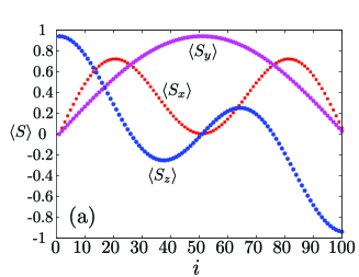
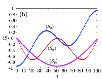
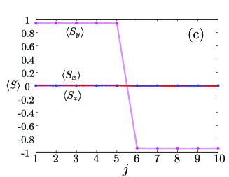
Figure 2: The spatial variations of $\langle{\bf S}_{i,j}\rangle$ for $D=0.5$, $\alpha=0.04$ and $T=0.2T_{C}$. (a) $j=1$, (b) $j=10$ and (c) $i=51$. Note that $(x,y,z)$ is the absolute coordinate system.

It means that a domain wall is formed along the circumference of the Möbius strip as schematically shown in Fig.3(a), and we call this kind of DW as type-A . When we transform $S^{\mu}_{i,j}$ (absolute coordinate) to ${\tilde{S}}^{\mu}_{i,j}$ (relative coordinate), the latter has only ${\tilde{z}}$ component except near the DW.

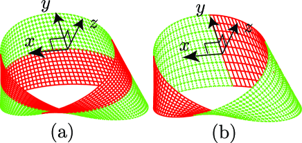
Figure 3: Two types of domain walls: (a) type A - parallel to the circumference and (b) type B - perpendicular to it. $(x,y,z)$ are the axes of the absolute coordinate system.

Next we consider the case of stronger inter-chain coupling, $\alpha=0.15$. In Fig.4(a) the $i$ dependence of $\langle S^{\mu}_{i,j}\rangle$ is shown for $j=1$ and $j=10$ for $T=0.2T_{C}$ ($T_{C}=0.883J$). (The results for $j=1$ and $j=10$ are the same.) In this case $\langle S^{\mu}_{i,j}\rangle$ for $i=N_{x}$ in the $j=1$ chain do not connect smoothly to those for $i=1$ in the $j=10$, and so the discontinuity is observed. On the other hand the $j$ dependence is smooth [Fig.4(b)], and this behavior is the same for all $i$.

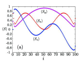
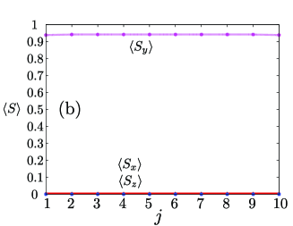
Figure 4: The spatial variations of $\langle{\bf S}_{i,j}\rangle$ for $D=0.5$, $\alpha=0.15$ and $T=0.2T_{C}$. (a) $j=1$, and (b) $i=51$.

It indicates that the DW is located perpendicularly to the circumference in contrast to the case of $\alpha=0.04$, and we call this kind of DW as type B [schematically shown in Fig.3(b)]. Naively we expect that a type-A (B) domain wall is stable if $N_{x}\alpha<N_{y}$ ($N_{x}\alpha>N_{y}$), since the energy to create a DW is smaller compared to that for type B (A). The results shown in Figs.2 and 4 are consistent with this expectation.

However, this stability condition for DWs will not hold at higher temperatures or reduced values of $D$. In Fig.5 the phase diagram in the plane of $\alpha$ and $T$ is shown.

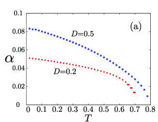
Figure 5: Phase diagram in the plane of $T$ and $\alpha$. Curves are the boundaries between type-A and B domain walls, and the region close to the origin corresponds to the type-A domain wall.

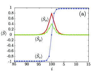
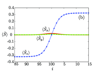
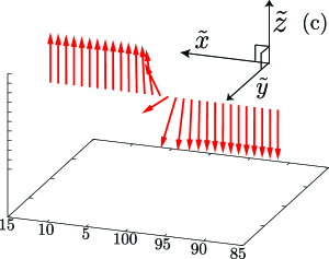
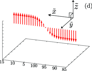
Figure 6: The spatial variations of $\langle{\tilde{\bf S}}_{i,j}\rangle$ near the DW in the relative coordinate system for $D=0.5$ and $\alpha=0.15$. $T=0.1T_{C}$ for (a) and (c), and $T=0.9T_{C}$ for (b) and (d).

As seen the region of type-B domain wall becomes larger as $T$ is increased or $D$ is decreased. This behavior can be understood as follows. Since we consider the quasi-one-dimensional system, the inter-chain exchange interaction $J\alpha$ is much smaller than the intra-chain exchange $J$. The single-ion anisotropy energy $D$ was taken to be $J\alpha<D<J$, which seems to be a natural choice. Since the $D$ term favors the spin alignment normal to the strip, the loss of energy would become large for the broader width of the DW of type A. Then the width of the type-A DW is quite small irrespective of the temperature, actually a single site in most cases. On the contrary for the type-B DW, the width of the DW may become large because $D<J$. As $D$ is further decreased or the temperature is increased, the width of DW can be larger and so the DW formation energy becomes smaller.chikazumi The spatial variations of $\langle{\tilde{S}}_{i,j}^{\alpha}\rangle$ (in the relative coordinate system) for $85\leq i\leq 100$ and $1\leq i\leq 15$ are depicted in Fig.6. The width of the type-B DW is actually smaller at lower $T$ for the same value of $D$. Here $\langle{\tilde{S}}_{i,j}^{\alpha}\rangle$ for $85\leq i\leq 100$ are multiplied by -1, since the normal direction in the relative coordinate system is reversed between the sites with $i=100$ and $i=1$. We have also checked that the width becomes larger for smaller $D$ at the same temperature, as stated above. Thus the type-B DW becomes favorable compared to type-A DW, as $T$ is increased or $D$ is decreased.

From Fig.5 we see that the phase transition from type-B DW to type-A DW occurs as the temperature $T$ is lowered. This results in an interesting behavior of the magnetization as a function of $T$. In Fig.7 the $T$ dependences of the magnetizations for $\alpha=0.15$ and $\alpha=0.04$ are shown, where the total magnetization for each direction, $M_{\mu}$ ($\mu=x,y,z$), and its magnitude, $M_{tot}$, are defined as

$$\begin{array}[]{rl}M_{\mu}=&\displaystyle\frac{1}{N_{x}N_{y}}\sum_{i=1}^{N_{x}}\sum_{j=1}^{N_{y}}\langle S^{\mu}_{i,j}\rangle,\\ M_{tot}=&\displaystyle\sqrt{M_{x}^{2}+M_{y}^{2}+M_{z}^{2}}.\end{array}$$ (8)

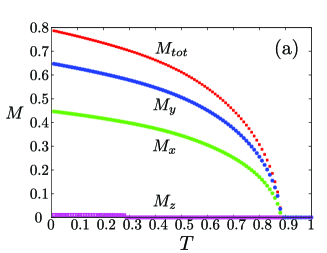
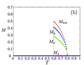
Figure 7: $T$ dependences of the magnetizations for $D=0.5$, (a) $\alpha=0.15$, and (b) $\alpha=0.04$. The magnetization has a jump as indicated by the dashed vertical line.

In the case of $\alpha=0.15$ the magnetization monotonously increases as $T$ is lowered. On the contrary the magnetization for $\alpha=0.04$ suddenly vanishes at $T\sim 0.6J$. This is because the phase transition from type-B DW to type-A DW occurs at this temperature. If the DW is of type A, the magnetizations in the $j$ th chain are exactly canceled by those in the $(N_{y}-j+1)$ th chain, though locally there are finite magnetizations. On the other hand, in the case of type-B DW there is no such cancellation and the total magnetization is finite, and it becomes larger as $T$ is lowered. In realistic systems this behavior of the magnetization would be observed with the hysteresis. However, the detection of this behavior may be difficult because type-A and type-B DW states have globally different structures so that the pinning of DWs due to impurities or dislocations would disturb their motion more seriously than usual cases.

The Curie temperature for the system with Möbius geometry is only slightly lower than that for the planar system with the same parameters. For $D=0.5$, $\alpha=0.04$, $N_{x}=100$, and $N_{y}=10$, the former is $0.811J$ while the latter is $0.812J$. (The $T_{C}$ for the infinite plane with the same $D$ and $\alpha$ is $0.813J$.) When $N_{x}$ and $N_{y}$ become larger the difference of $T_{C}$ will be smaller, since the local curvature of the Möbius strip is decreasing. This implies that the Curie temperature for the Möbius system is close to that for the flat system in general, at least in the mean-field approximation.

IV effect of external magnetic field

Next we examine the effect of an external magnetic field ${\bf H}$ on the domain-wall structure. Here ${\bf H}$ is assumed to be applied along the $y$ direction, i.e., ${\bf H}$ threads the Möbius strip. The $T$ dependences of the magnetizations are shown in Fig.8. Because of finite $H$, the magnetization is finite for $T>T_{C}(H=0)$ and gradually decreases as $T$ is increased.

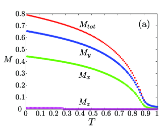
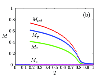
Figure 8: $T$ dependences of the magnetizations for $D=0.5$, $H=0.01$, (a) $\alpha=0.15$, and (b) $\alpha=0.04$. The magnetization has a jump as indicated by the dashed vertical line.

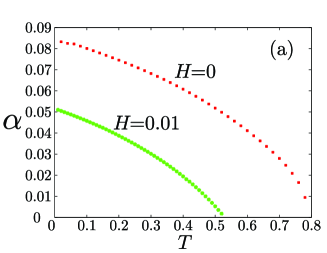
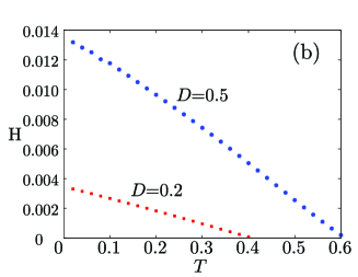
Figure 9: Phase diagram (a) in the plane of $\alpha$ and $T$ with $D=0.5$, and (b) in the plane of $H$ and $T$ with $\alpha=0.04$. Curves are the boundaries between type-A and B domain walls, and the region close to the origin corresponds to the type-A domain wall.

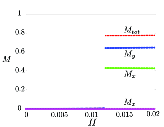
Figure 10: Magnetization as a function of the external field $H$ for $D=0.5$, $\alpha=0.04$, and $T=0.1T_{C}$. The magnetization has a jump as indicated by the dashed vertical line.

For $\alpha=0.15$ [Fig.8(a)] the magnetization smoothly grows as $T$ is decreased for $T<T_{C}(H=0)$, while there is a discontinuity in the case of $\alpha=0.04$ [Fig.8(b)]. This is again due to the transition from type-B to type-A DW, but the transition occurs at a much lower temperature compared to the case of $H=0$ [Fig.7(b)]. This is because the Zeeman coupling lowers the energy of the state with type-B DW due to its finite total magnetization and type-B state is more favored in the presence of the external field. For $H\not=0$ the magnetization in the type-A state is finite but is very small. Next we show the phase diagram in the plane of $T$ and $\alpha$ for fixed value of $H$ [Fig.9(a)] and that in the plane of $T$ and $H$ for fixed $\alpha$ [Fig.9(b)]. In both Figs.9(a) and 9(b) the region of type-A DW shrinks when $H$ is applied. This can be understood similarly as the $T$ dependence of the magnetization. In the type-B state the magnetization is already finite without $H$, so that the energy can be gained due to the coupling to the applied magnetic field. Then the type-B state is more favorable compared to the type-A state in the presence of $H$. This resulted in a serious difference in response to the applied magnetic field for two types of DWs. The dependence of the magnetization on the external magnetic field is shown in Fig.10. There is again a jump of the magnetization as a function of $H$ because of the transition between different types of DWs. If we assume $J\sim$10meV, the transition point locates at around $H$=1T for the parameters used here.

In the above we have assumed that ${\bf H}$ is applied along the $y$ direction. For the type-B DW, this direction is parallel to the domain wall. When ${\bf H}$ is applied along other directions, type-B DW will move to a different position at which the more Zeeman energy can be gained. This problem will be examined elsewhere.

V summary

In summary, we have studied the structure of domain walls in ferromagnetic Möbius strips. We found that there can be two kinds of domain walls whose relative stability is quite sensitive to the change in temperature and the applied magnetic field. The magnetizations will have interesting behaviors in that they have discontinuities as functions of both temperature and the magnetic field. Although ferromagnetic Möbius strips have not yet been obtained, we expect that these systems will attract much interest both theoretical and experimental once they are synthesized.

- (1) S. Tanda, H. Kawamoto, M. Shiobara, Y. Okajima, and K. Yamaya, J. Phys, IV 9, Pr10-379 (1999).
- (2) S. Tanda, H. Kawamoto, M. Shiobara, Y. Sakai, S. Yasuzuka, Y. Okajima, and K. Yamaya, Physica B 284-288, 1657 (2000).
- (3) Y. Okajima, H. Kawamoto, M. Shiobara, K. Matsuda, S. Tanda, and K. Yamaya, Physica B 284-288, 1659 (2000).
- (4) S. Tanda, T. Tsuneta, Y. Okajima, K. Inagaki, K. Yamaya, and N. Hatakenaka, Nature (London) 417, 397 (2002).
- (5) M. Hayashi and H. Ebisawa, J. Phys. Soc. Jpn. 70, 3495 (2001).
- (6) M. Hayashi, H. Ebisawa and K. Kuboki, Phys. Rev. B 72, 024505 (2005)
- (7) T. Nogawa and K. Nemoto, Phys. Rev. B 73, 184504 (2006) .
- (8) M. Hayashi, H. Ebisawa, and K. Kuboki, Europhys. Lett. 76(2), 264 (2006)
- (9) M. Hayashi, H. Ebisawa, and K. Kuboki, Phys. Rev. B 76, 014303 (2007) .
- (10) K. Yakubo, Y. Avishai, and D. Cohen, Phys. Rev. B 67, 125319 (2003).
- (11) F. Mila, C. A. Stafford, and S. Caponi, Phys. Rev. B 57, 1457 (1998).
- (12) K. Wakabayashi and K. Harigaya, J. Phys. Soc. Jpn. 72, 998 (2003).
- (13) K. Kaneda and Y. Okabe, Phys. Rev. Lett. 86, 2134 (2001).
- (14) N. D. Mermin and H. Wagner, Phys. Rev. Lett. 17, 1133 (1966).
- (15) S. Chikazumi, Physics of Ferromagnetism, (Oxford University Press, New York, 1997).