Test of the Littlest Higgs model through the correlation
among $W$ boson, top quark and Higgs masses

Abstract

Motivated by the recent precision measurements of the $W$ boson mass and top quark mass, we test the Littlest Higgs model by confronting the prediction of $M_{{}_{W}}$ with the current and prospective measurements of $M_{{}_{W}}$ and $M_{t}$ as well as through the correlation among $M_{{}_{W}}$, $M_{t}$ and Higgs mass. We argue that the current values and accuracy of $M_{{}_{W}}$ and $M_{t}$ measurements tend to favor the Littlest Higgs model over the standard model, although the most recent electroweak data may appear to be consistent with the standard model prediction. In this analysis, the upper bound on the global $SU(5)$ symmetry breaking scale turned out to be 26.3 TeV. We also discuss how the masses of the heavy gauge boson $M_{B^{{}^{\prime}}}$ in the Littlest Higgs model can be predicted from the constraints on the model parameters.

PACS Numbers: 12.15.Lk, 12.60.Cn, 14.80.Cp

I Introduction

There have been a great deal of works on the precision test of the standard model (SM) because of the incredibly precise data obtained at the LEP and the new measurements of $M_{{}_{W}}$ and $M_{t}$ at the Fermilab Tevatron :2007ypa ; Group:2008nq as well as the recent theoretical progress in the higher order radiative corrections Buttar:2006zd . With such a dedicated effort for a long time to test the SM, it has been confirmed that the SM is the right model to describe the electroweak phenomena at the current experimental energy scale. What remains elusive is the origin of the electroweak symmetry breaking for which a Higgs boson is responsible in the SM. It has been known for some time that radiative corrections in the SM exhibit a small but important dependence on the Higgs boson mass, $M_{h}$. As a result, the value of $M_{h}$ can, in principle, be predicted by comparing a variety of precision electroweak measurements with one another. The recent global fits to all precision electroweak data (see J. Erler and P. Langacker PDG ) lead to $M_{h}=113^{+56}_{-40}$ ($1\sigma$ confidence level (CL)) and $M_{h}<241$ GeV ($95\%$ CL). Those constraints are very consistent with bounds from direct searches for the Higgs boson at LEPII via $e^{+}+e^{-}\longrightarrow Zh$, $M_{h}>114.4$ GeV Barate:2003sz . Together, they seem to suggest the range, 114 GeV $<M_{h}<$ 241 GeV, and imply very good consistency between the SM and experiment. However, in the context of the SM valid all the way up to the Planck scale, $M_{h}$ diverges due to a quadratic divergence at one loop level unless it is unnaturally fine-tuned. Thus, we need a new physics beyond the SM to stabilize $M_{h}$, which is a so-called hierarchy problem that has motivated the construction of the LHC. Candidates for this physics include supersymmetry and technicolor models relying on strong dynamics to achieve electroweak symmetry breaking.

Inspired by dimensional deconstruction ArkaniHamed:2001ca , an intriguing alternative possibility that the Higgs boson is a pseudo Goldstone boson  Georgi:1974yw ; ArkaniHamed:2002qy has been revived by Arkani-Hamed et al.. They showed that the gauge and Yukawa interactions of the Higgs boson can be incorporated in such a way that a quadratically divergent one-loop contribution to $M_{h}$ is canceled. The cancelation of this contribution occurs as a consequence of the special collective pattern in which the gauge and Yukawa couplings break the global symmetries. Since the remaining radiative corrections to $M_{h}$ are much smaller, no fine tuning is required to keep the Higgs boson sufficiently light if the strong coupling scale is of order 10 TeV. Such a light Higgs boson was called “little Higgs”. The models with little Higgs are described by nonlinear sigma models and trigger electroweak symmetry breaking by the collective symmetry breaking mechanism. Many such models with different “theory space” have been constructed  ArkaniHamed:2002qy ; Schmaltz:2004de , and electroweak precision constraints on various little Higgs models have been investigated by performing global fits to the precision data  Csaki:2002qg ; Csaki:2003si ; Deandrea:2004qq . It is worthwhile to notice that the little Higgs models generally have three significant scales: an electroweak scale $v\sim\frac{g^{2}f}{4\pi}\sim$ 200 GeV, a new physics scale $g\cdot f$ $\sim$ 1 TeV and a cut-off scale of the non-linear sigma model $\Lambda$ $\sim$ $4\pi f$ $\sim$ 10 TeV, where $f$ is the scale of the global symmetry breaking. Therefore, we expect that the little Higgs models have rich and distinguishable TeV scale phenomena unlike other models, which provides strong motivation to probe them at the LHC.

Very recently, Fermilab CDF collaboration has reported the most precise single measurement of the $W$ boson mass to date from Run II of the Tevatron  :2007ypa ,

$$M_{{}_{W}}=80.413\pm 0.048~{}\mbox{GeV},$$ (1)

and updated the world average Alcaraz:2007ri to

$$M_{{}_{W}}=80.398\pm 0.025~{}\mbox{GeV}.$$ (2)

In addition, the world average result of $M_{t}$ from the Tevatron experiments CDF and D0 has been given Group:2008nq by

$$M_{t}=172.6\pm 1.4~{}\mbox{GeV}.$$ (3)

The mass of the top quark is now known with a relative precision of $0.8\%$, limited by the systematic uncertainties, and can be reasonably expected that with the full Run-II data set the top-quark mass will be known to much better than $0.8\%$ in the foreseeable future. With the current level of experimental uncertainties as well as prospective sensitivities on $M_{{}_{W}}$ and $M_{t}$, we are approaching to the level to test the validity of new physics beyond the SM by a direct comparison with data or to strongly constrain new physics models.

The correlation among $M_{t}$, $M_{{}_{W}}$ and $M_{h}$ is an important prediction of the SM, and thus deviations from it should be accounted for by the effects of new physics. In the minimal supersymmetric standard model (MSSM) case, the allowed ranges for $M_{{}_{W}}$ and $M_{t}$ were checked by considering various parameter spaces of the MSSM Heinemeyer:2006nm . They showed that the previous experimental results for $M_{{}_{W}}$ and $M_{t}$ tend to favor the MSSM over the SM. Motivated by this fact, in this letter, we confront the Littlest Higgs model (LHM) ArkaniHamed:2002qy with more precision measurements of $M_{{}_{W}}$ and $M_{t}$ than before by computing the prediction of $M_{{}_{W}}$ in the LHM. We examine whether the current precision measurements of $M_{{}_{W}}$ and $M_{t}$ tend to favor the LHM over the SM or not. From the careful numerical analysis, we obtain some constraints on the model parameters such as the global $SU(5)$ symmetry breaking scale and the mixing angles between heavy gauge bosons. By using the constraints on the model parameters, we show how the mass of heavy gauge boson $B^{\prime}_{\mu}$ can be predicted, which could be probed at the LHC.

The organization of this letter is as follows. In Sec. II we briefly review the LHM. In Sec. III we discuss how the formula for $M_{{}_{W}}$ can be derived from the effective theory of the LHM, and confront the prediction of $M_{{}_{W}}$ with the current and prospective measurements of $M_{{}_{W}}$ and $M_{t}$. We also show how an upper bound on the global symmetry breaking scale $f$ can be obtained and how it is correlated with the Higgs mass. In Sec. IV we investigate how the mixing parameters in the LHM can be constrained, and discuss how the mass of the heavy gauge boson $B^{{}^{\prime}}_{\mu}$ in the LHM can be predicted from the constraints on the model parameters. Finally we conclude our work.

II Aspects of the littlest Higgs model

We start with reviewing the aspects of the LHM which are relevant to our work. The LHM is one of the simplest and phenomenologically viable models, which realizes little Higgs idea. It initially has a global symmetry $SU(5)$ which is broken down to a global symmetry $SO(5)$ via a vacuum expectation value of order $f$, and a gauge group $[SU(2)\times U(1)]^{2}$ which is broken down to $SU(2)\times U(1)$, identified as the electroweak gauge symmetry. The characteristic feature of the LHM is to predict the existence of the new gauge bosons with masses of order TeV. The vacuum expectation value (VEV) associated with the spontaneous global symmetry breaking of $SU(5)$ is proportional to the $5\times 5$ symmetric matrix $\Sigma_{0}$ given by

$$\Sigma_{0}=\left(\begin{array}[]{ccccc}&&&1&\\ &&&&1\\ &&1&&\\ 1&&&&\\ &1&&&\\ \end{array}\right).$$ (4)

The global symmetry breaking yields 14 Goldstone bosons which transform under the electroweak $SU(2)$ symmetry as a real singlet, a real triplet, a complex doublet and a complex triplet:

$$\mathbf{14}=\mathbf{1}_{0}+\mathbf{3_{0}}+\mathbf{2_{\pm_{1/2}}}+\mathbf{3_{\pm_{1/2}}}~{}.$$ (5)

Among them four massless Goldstone bosons, $\mathbf{1}_{0}$ and $\mathbf{3_{0}}$ are eaten by the gauge fields so that the gauge symmetry $[SU(2)\times U(1)]^{2}$ is broken down to its diagonal subgroup $SU(2)\times U(1)$. The remaining complex doublet $\textbf{2}_{\pm 1/2}$ and triplet $\textbf{3}_{\pm 1/2}$ are identified as a component of the SM Higgs sector and an extra complex triplet Higgs, respectively. The generators of the gauge symmetry embedded into $SU(5)$ are given by

$$Q^{a}_{1}=\left(\begin{array}[]{ccc}\sigma^{a}/2&0&0\\ 0&0&0\\ 0&0&0\\ \end{array}\right),~{}~{}~{}Y_{1}={\rm diag}(-3,-3,2,2,2)/10,$$ (6)

$$Q^{a}_{2}=\left(\begin{array}[]{ccc}0&0&0\\ 0&0&0\\ 0&0&-\sigma^{a*}/2\\ \end{array}\right),~{}~{}~{}~{}Y_{2}={\rm diag}(-2,-2,-2,3,3)/10,$$ (7)

where $\sigma^{a}$ are the Pauli spin matrices and $Q^{a}_{i}$ and $Y_{i}$ are each $SU(2)$ and $U(1)$ generators, respectively. Then, the generators of the electroweak symmetry $SU(2)_{L}\times U(1)_{Y}$ are $Q^{a}=(Q^{a}_{1}+Q^{a}_{2})/\sqrt{2}$ and $Y=Y_{1}+Y_{2}$.

The fluctuations of the remaining Goldstone bosons in the broken direction can be described by $\Pi=\pi^{a}X^{a}$ with the broken generators of the $SU(5)$, $X^{a}$ . Then the Goldstone bosons can be parameterized by a nonlinear sigma model field $\Sigma(x)$,

$$\Sigma(x)=e^{i\Pi/f}\Sigma_{0}e^{i\Pi^{T}/f}=e^{2i\Pi/f}\Sigma_{0}.$$ (8)

In terms of uneaten fields, the Goldstone boson field, $\Pi$, is given by

$$\Pi=\left(\begin{array}[]{ccc}0&\frac{H^{\dagger}}{\sqrt{2}}&\Phi^{\dagger}\\ \frac{H}{\sqrt{2}}&0&\frac{H^{\ast}}{\sqrt{2}}\\ \Phi&\frac{H^{T}}{\sqrt{2}}&0\end{array}\right),$$ (9)

where $H$ denotes the little Higgs doublet $(h^{0},h^{\dagger})$ and $\Phi$ is a complex triplet scalar field. We note that the triplet scalar field $\Phi$ should have a small expectation value of order GeV in order to not give too large contribution to the $T$ parameter Csaki:2002qg .

The kinetic energy term of the nonlinear sigma field $\Sigma$ is given by

$$\frac{f^{2}}{8}TrD_{\mu}\Sigma\cdot(D^{\mu}\Sigma)^{\dagger},$$ (10)

where the covariant derivative of $\Sigma$ is

$$D_{\mu}\Sigma=\partial_{\mu}\Sigma-i\Sigma_{j}[g_{j}W^{a}_{j\mu}(Q^{a}_{j}\Sigma+\Sigma Q^{a\,T}_{j})+g^{{}^{\prime}}_{j}B_{j\mu}(Y_{j}\Sigma+\Sigma Y_{j})],$$ (11)

with $j=1,2$. Here $W^{a}_{j\mu}$ and $B_{j\mu}$ stand for the $SU(2)$ and $U(1)$ gauge fields, respectively and $g_{j}$ and $g^{\prime}_{j}$ denote the corresponding gauge coupling constants.

It is convenient to expand $\Sigma$ around the VEV in powers of $1/f$,

$$\Sigma=\Sigma_{0} + \frac{2i}{f}\left(\begin{array}[]{ccc}\Phi^{\dagger}&\frac{H^{\dagger}}{\sqrt{2}}&\mathrm{0}_{2\times 2}\\ \frac{H^{*}}{\sqrt{2}}&0&\frac{H}{\sqrt{2}}\\ \mathrm{0}_{2\times 2}&\frac{H^{T}}{\sqrt{2}}&\Phi\end{array}\right)$$ (15)

$$- \frac{1}{f^{2}}\left(\begin{array}[]{ccc}H^{\dagger}H^{*}&\sqrt{2}\Phi^{\dagger}H^{T}&H^{\dagger}H+2\Phi^{\dagger}\Phi\\ \sqrt{2}H\Phi^{\dagger}&2HH^{\dagger}&\sqrt{2}H^{*}\Phi\\ H^{T}H^{*}+2\Phi\Phi^{\dagger}&\sqrt{2}\Phi H^{\dagger}&H^{T}H\end{array}\right)$$

$$+ \textit{O}\left(\frac{1}{f^{3}}\right).$$

Inserting Eq. (II) into Eq. (11), we obtain the mixing terms between gauge bosons as follows,

$$\mathcal{L}_{\Sigma,~{}\rm LO} \sim \frac{f^{2}}{8}\,\mathrm{Tr}|\,\Sigma_{j=1,2}[\,g_{j}W_{j\,\mu}^{a}(Q_{j}^{a}\Sigma_{0}+\Sigma_{0}Q^{aT}_{j})+g^{{}^{\prime}}_{j}B_{j\,\mu}(Y_{j}\Sigma_{0}+\Sigma_{0}Y_{j})]\,|^{2}$$

$$\sim \frac{f^{2}}{8}\{\left(g_{1}^{2}W_{1\,\mu}^{a}W_{2}^{a\mu}-2g_{1}g_{2}W_{1\,\mu}^{a}W_{2}^{a\mu}+g_{2}^{2}W_{2\,\mu}^{a}W_{2}^{a\mu}\right)$$

$$+\frac{1}{5}\left(\,g_{1}^{{}^{\prime}2}B_{1\,\mu}B_{1}^{\mu}-2g_{1}^{{}^{\prime}}g_{2}^{{}^{\prime}}B_{1\,\mu}B_{2}^{\mu}+g_{2}^{{}^{\prime}2}B_{2\,\mu}B_{2}^{\mu}\right)\}.$$

With the help of the following transformations

$$W^{a}_{\mu}=sW^{a}_{1\,\mu}+cW^{a}_{2\,\mu}~{},~{}~{}~{}W^{a^{\prime}}_{\mu}=-cW^{a}_{1\,\mu}+sW^{a}_{2\,\mu},$$ (21)

$$B_{\mu}=s^{{}^{\prime}}B_{1\,\mu}+c^{{}^{\prime}}B_{2\,\mu}~{},~{}~{}~{}B^{{}^{\prime}}_{\mu}=-c^{{}^{\prime}}B_{1\,\mu}+s^{{}^{\prime}}B_{2\,\mu},$$ (22)

with

$$s=\frac{g_{2}}{\sqrt{g_{1}^{2}+g_{2}^{2}}}~{},~{}~{}~{}c=\frac{g_{1}}{\sqrt{g_{1}^{2}+g_{2}^{2}}},$$ (23)

$$s^{{}^{\prime}}=\frac{g_{2}^{{}^{\prime}}}{\sqrt{g_{1}^{{}^{\prime}2}+g_{2}^{{}^{\prime}2}}}~{},~{}~{}~{}c^{{}^{\prime}}=\frac{g_{1}^{{}^{\prime}}}{\sqrt{g_{1}^{{}^{\prime}2}+g_{2}^{{}^{\prime}2}}},$$ (24)

two massive states $W^{a\prime}_{\mu}$ and $B^{\prime}_{\mu}$ are obtained whose masses are given by

$$M_{W^{a^{\prime}}_{\mu}}=\sqrt{g_{1}^{2}+g_{2}^{2}}\,\frac{f}{2},$$

$$M_{B^{{}^{\prime}}_{\mu}}=\sqrt{g_{1}^{{}^{\prime}2}+g_{2}^{{}^{\prime}2}}\frac{f}{\sqrt{20}},$$ (25)

respectively, and two massless $W^{a}_{\mu}$ and $B_{\mu}$ bosons which are identified as the massless SM gauge bosons before the electroweak symmetry breaking. Those SM gauge fields become massive after the electroweak symmetry breaking at a few hundred GeV scale. Hereafter we denote the SM gauge fields in the mass basis as $W,Z$ and $A$. We also notice that the SM gauge couplings are $g=g_{1}s=g_{2}c$ and $g^{\prime}=g^{\prime}_{1}\,s^{\prime}=g^{\prime}_{2}\,c^{\prime}$ for $SU(2)_{L}$ and $U(1)_{Y}$, respectively.

III Prediction of $M_{{}_{W}}$ and upper bound on $f$

The primary goal of our work is to estimate the prediction for the mass of $W$ boson in the LHM. To do this, it is convenient to construct low energy effective lagrangian for the LHM below the mass scales of the heavy gauge bosons and then extract the corrections coming from higher dimensional operators. The quartic couplings of the Higgs and gauge bosons can be obtained by expanding the next-to-leading order terms of the non-linear sigma field in the kinetic term,

$$\mathcal{L}_{\Sigma,~{}\rm NLO} \sim \frac{1}{2}\mathrm{Tr}|\,\Sigma_{j=1,2}[\,g_{j}W_{j\mu}^{a}(Q_{j}^{a}\Pi\Sigma_{0}+\Pi\Sigma_{0}Q^{aT}_{j})+g^{{}^{\prime}}_{j}B_{j\mu}(Y_{j}\Pi\Sigma_{0}+\Pi\Sigma_{0}Y_{j})]\,|^{\,2}.$$ (26)

Expressing these gauge bosons in terms of the mass eigenstates $W_{\mu}^{a},~{}W^{a^{\prime}}_{\mu},~{}B_{\mu}$ and $B^{{}^{\prime}}_{\mu}$, the quartic terms are given by

$$\mathcal{L}_{\Sigma,~{}\rm NLO} \sim +\frac{1}{4}g^{2}\left(W_{\mu}^{a}W^{b\,\mu}-\frac{(c^{2}-s^{2})}{sc}W_{\mu}^{a}W^{\prime\,b\,\mu}\right)\mathrm{Tr}[H^{\dagger}H\delta^{ab}+2\Phi^{\dagger}\Phi\,\delta^{ab}+2\sigma^{a}\Phi^{\dagger}\sigma^{b\,T}\Phi]$$ (27)

$$-\frac{1}{4}g^{2}\left(W_{\mu}^{\prime\,a}W^{\prime\,a\,\mu}\,\mathrm{Tr}[H^{\dagger}H+2\Phi^{\dagger}\Phi]-\frac{(c^{4}+s^{4})}{2s^{2}c^{2}}W_{\mu}^{\prime\,a}W^{\prime\,b\mu}\,\mathrm{Tr}[2\sigma^{a}\Phi^{\dagger}\sigma^{bT}\Phi]\right)$$

$$+g^{\prime\,2}\left(B_{\mu}B^{\mu}-\frac{(c^{\prime\,2}-s^{\prime\,2})}{s^{\prime}c^{\prime}}B_{\mu}B^{\prime\,\mu}\right)\,\mathrm{Tr}[\frac{1}{4}H^{\dagger}H+\Phi^{\dagger}\Phi]$$

$$-g^{\prime\,2}\left(B^{\prime}_{\mu}B^{\prime\,\mu}\,\mathrm{Tr}[\frac{1}{4}H^{\dagger}H]-\frac{(c^{\prime\,2}-s^{\prime\,2})^{2}}{4s^{\prime\,2}c^{\prime\,2}}B^{\prime}_{\mu}B^{\prime\,\mu}\mathrm{Tr}[\Phi^{\dagger}\Phi]\right)+\dots~{}.$$

Integrating out the heavy gauge bosons $W^{a^{\prime}}_{\mu}$ and $B^{{}^{\prime}}_{\mu}$, we obtain additional operators which cause modification of relations between the SM parameters, and thus their coefficients can be constrained from electroweak precision data. Among the additional operators, the terms quadratic with respect to the light gauge fields are given in the unitary gauge by

$$\mathcal{L}_{~{}\rm effective} \sim -\frac{g^{2}(s^{2}-c^{2})^{2}}{8f^{2}}W^{a\,\mu}W^{a}_{\mu}h^{4}-\frac{5g^{2}(s^{\prime\,2}-c^{\prime,2})^{2}}{8f^{2}}W^{3\mu}W^{3}_{\mu}h^{4}$$ (28)

$$-\frac{g^{\prime\,2}(s^{2}-c^{2})^{2}}{8f^{2}}B^{\mu}B_{\mu}h^{4}-\frac{5g^{\prime\,2}(s^{\prime\,2}-c^{\prime\,2})^{2}}{8f^{2}}B^{\mu}B_{\mu}h^{4}$$

$$+\frac{gg^{\prime}(s^{2}-c^{2})^{2}}{4f^{2}}W^{3\mu}B_{\mu}h^{4}$$

$$+\frac{g^{2}}{4f^{2}}W^{a\mu}W^{a}_{\mu}h^{4}+\frac{g^{\prime\,2}}{4f^{2}}B^{\mu}B_{\mu}h^{4}-\frac{gg^{\prime}}{2f^{2}}B^{\mu}W^{3}_{\mu}h^{4}$$

$$+\frac{g^{2}}{2}W^{a\mu}W^{a}_{\mu}\varphi^{2}+\frac{g^{2}}{2}W^{3\mu}W^{3}_{\mu}\varphi^{2}+g^{\prime\,2}B^{\mu}B_{\mu}\varphi^{2}-2gg^{\prime}B^{\mu}W^{3}_{\mu}\varphi^{2},$$

where we only take the $h~{}\equiv{\rm Re}~{}h^{0}$ component of Higgs field $H$ and $\varphi~{}\equiv{\rm Re}~{}\phi^{0}$ component of the triplet scalar field $\Phi$ from the lagrangian above up to $\frac{v^{4}}{f^{2}}$ order. Those operators in Eq. (28) induce corrections to the masses of $W$ and $Z$ bosons after the scalar fields get VEVs. After $h$ and $\varphi$ get VEVs

$$<h>=\frac{v}{\sqrt{2}},$$ (29)

$$<\varphi>={v^{\prime}},$$ (30)

we obtain the masses of $W$ and $Z$ bosons and fermi constant $G_{F}$, which are presented in terms of the model parameters as follows;

$$M_{{}_{W}}^{2} = g^{2}\frac{v^{2}}{4}\left(1+\frac{(s^{4}+6s^{2}c^{2}+c^{4})v^{2}}{4f^{2}}+4\frac{v^{{}^{\prime}2}}{v^{2}}\right)~{},$$ (31)

$$M_{{}_{Z}}^{2} = (g^{2}+g^{{}^{\prime}2})\frac{v^{2}}{4}\left(1+\frac{(s^{4}+6s^{2}c^{2}+c^{4})v^{2}}{4f^{2}}-\frac{5(s^{{}^{\prime}2}-c^{{}^{\prime}2})^{2}v^{2}}{4f^{2}}+8\frac{v^{{}^{\prime}2}}{v^{2}}\right)~{},$$ (32)

$$\frac{1}{G_{F}} = \sqrt{2}v^{2}\left(1+\frac{v^{2}}{4f^{2}}+4\frac{v^{{}^{\prime}2}}{v^{2}}\right)~{}.$$ (33)

Now, let us relate the model parameters to observables by using the precision experimental values of $\alpha(M^{2}_{{}_{Z}}),M_{{}_{Z}}$ and $G_{F}$ as inputs. From the standard definition of the weak mixing angle $\sin\theta_{0}$ around the $Z$ pole given as follows Peskin:1991sw ,

$$\sin^{2}\theta_{0}\cos^{2}\theta_{0} = \frac{\pi\alpha(M^{2}_{{}_{Z}})}{\sqrt{2}G_{F}M^{2}_{{}_{Z}}}~{},$$ (34)

$$\sin^{2}\theta_{0} = 0.23108\pm 0.00005~{},$$ (35)

where $\alpha(M^{2}_{{}_{Z}})^{-1}=128.91\pm 0.02$ is the running SM fine-structure constant evaluated at $M_{{}_{Z}}$ PDG , we see that the mixing angle $\sin\theta_{W}$ is related to $\sin\theta_{0}$ through the relation,

$$s^{2}_{0} = s^{2}_{W}+\delta s^{2}_{W}=s^{2}_{W}-\frac{s^{2}_{W}c^{2}_{W}}{c^{2}_{W}-s^{2}_{W}}\left[\frac{\delta G_{F}}{G_{F}}+\frac{\delta{M^{2}_{{}_{Z}}}}{M^{2}_{{}_{Z}}}-\frac{\delta\alpha}{\alpha}\right]~{}$$ (36)

$$= s^{2}_{W}-\frac{s^{2}_{W}c^{2}_{W}}{c^{2}_{W}-{s^{2}_{W}}}\left[~{}4\Delta^{{}^{\prime}}+\Delta\left(-\frac{5}{4}+c^{2}(1-c^{2})+5c^{{}^{\prime}}(1-c^{{}^{\prime}2})\right)~{}\right]~{},$$

where

$$\Delta=\frac{v^{2}}{f^{2}}~{},~{}~{}~{}~{}~{}~{}\Delta^{{}^{\prime}}=\frac{v^{{}^{\prime}2}}{v^{2}}~{}.$$ (37)

Here, we omitted the $\delta\alpha$ term since there is no $\alpha$ correction. Using the relations Eqs. (31,32,36), we obtain

$$\frac{M_{{}_{W}}^{2}}{M^{2}_{{}_{Z}}}-c_{0}^{2}=\frac{c^{2}_{W}}{c^{2}_{W}-s^{2}_{W}}\left[~{}\Delta\left(\frac{5}{4}c^{2}_{W}-s^{2}_{W}(c^{2}-c^{4})-5c^{2}_{W}(c^{{}^{\prime}2}-c^{{}^{\prime}4})\right)-\Delta^{{}^{\prime}}4c^{2}_{W}\right]~{}.$$ (38)

Finally we can get the form of $M_{{}_{W}}$ as a function of $c,c^{{}^{\prime}},f$, after substituting the numerical value of $s_{0}$, as

$$M_{{}_{W}}(c,c^{{}^{\prime}},f)=(M_{{}_{W}})_{\rm SM}~{}[1+\Delta\cdot{\cal G}(c,c^{{}^{\prime}},f)+\Delta^{{}^{\prime}}\cdot{\cal H}(c,c^{{}^{\prime}},f)]~{},$$ (39)

and for $f\geq 4$ TeV, approximately

$$M_{{}_{W}}\simeq(M_{{}_{W}})_{\rm SM}~{}[1+\Delta(0.89-0.21c^{2}+0.21c^{4}-3.6c^{{}^{\prime}2}+3.6c^{{}^{\prime}4})-2.9\Delta^{{}^{\prime}}]~{}.$$ (40)

Therefore, it is reasonable that the $W$ boson mass $M_{{}_{W}}$ is decomposed into the SM contribution $(M_{{}_{W}})_{\rm SM}$ and the shift due to new tree-level contributions in the LHM .

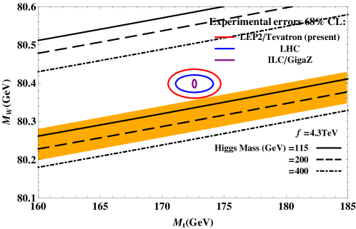
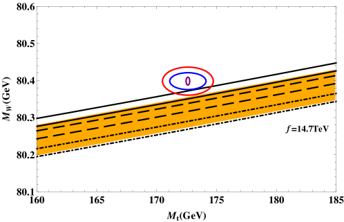
Figure 1: Plots represent maximum (upper line) and minimum (lower line) values of $M_{{}_{W}}$ as a function of $M_{t}$ in the SM (orange colored band) and the LHM with $f=4.3,~{}14.7$ and $26.3$ TeV, where solid, dashed and dot-dashed lines correspond to $M_{h}=115,~{}200$ and $400$ GeV, respectively. Red, blue and purple ellipses correspond to the current measurements  Alcaraz:2007ri ; Group:2008nq , prospective measurements at the LHC Beneke:2000hk ; Haywood:1999qg , and at the ILC with GigaZ Baur:2001yp ; Abe:2001nnb at the 68 $\%$ confidence level, respectively.

To compare the prediction of $W$ boson mass in the LHM with the current measurements of $M_{{}_{W}}$ and $M_{t}$, we first compute the SM contribution of the $W$-boson mass, $(M_{{}_{W}})_{\rm SM}$ by using the fortran program package $\rm ZFITTER$  Arbuzov:2005ma , in which two and three loop corrections are included. In the numerical estimation of $(M_{{}_{W}})_{\rm SM}$, we take the five parameters, hadronic correction to the QED coupling $\Delta^{(5)}_{h}$, the QCD coupling $\alpha_{\rm s}$, the $Z$ boson mass $M_{{}_{Z}}$, the top quark mass $M_{t}$ and the Higgs mass $M_{h}$, as input parameters. For their numerical values, we take $\Delta^{(5)}_{h}=0.02802(15)$, $\alpha_{\rm s}=0.1216(17)$, $M_{{}_{Z}}=91.1874(21)$ GeV. For the input values of $M_{t}$ and $M_{h}$, we consider the ranges $160\leq M_{t}\leq 185$ GeV and $115\leq M_{h}\leq 400$ GeV, respectively, in order to see how the prediction of $M_{{}_{W}}$ is correlated with $M_{t}$ and $M_{h}$. Here, the lower limit of $M_{h}$ is adopted from the direct search at LEP Barate:2003sz . As one can see from Eq. (40), the part of the shift of $M_{{}_{W}}$ from $(M_{{}_{W}})_{\rm SM}$ due to new contributions of the LHM depends on the parameters $c$, $c^{\prime}$, $\Delta$, and $\Delta^{\prime}$. For the sake of simplicity, we set the triplet VEV $v^{\prime}$ to be zero. We note in fact that this triplet VEV turns out to generate sub-leading contributions Csaki:2002qg . Thus, in this work, the model dependent input parameters are $c$, $c^{\prime}$ and $\Delta$. Among them, the parameters $c$ and $c^{\prime}$ are restricted to be $-1\leq c(c^{\prime})\leq 1$ and $\Delta$ should be much less than one. For example, if we take $f\simeq 1$ TeV, then $\Delta\simeq 0.06$.

Based on the formulae for $M_{{}_{W}}$ given in Eq. (40) and taking appropriate numerical values for the input parameters including $M_{t}$ and $M_{h}$, we finally obtain the prediction of $M_{{}_{W}}$ in the LHM. It is worthwhile to notice that there exist upper and lower limits for the prediction of $M_{{}_{W}}$ for a fixed parameter set ($M_{t},M_{h}$, $\Delta$) due to the restriction of the mixing parameters $c$ and $c^{\prime}$. As one can expect, the gap between the upper and lower limits for the prediction of $M_{{}_{W}}$ for a given $M_{h}$ gets smaller as the value of $f$ increases.

In Fig. 1, we show the predictions of $M_{{}_{W}}$ in the SM and the LHM with $f$=4.3, 14.7 and 26.3 TeV as a function of $M_{t}$. The reason why we take those particular values of $f$ will become clear from the discussions presented below. The orange colored bands in Fig. 1 indicate the SM prediction of $M_{{}_{W}}$ for $115~{}{\rm GeV}\leq M_{h}\leq 400~{}{\rm GeV}~{}$. As is well known, the SM prediction of $M_{{}_{W}}$ for a fixed $M_{t}$ gets smaller as $M_{h}$ increases, so the upper and lower limits for the orange bands correspond to $M_{h}=115$ GeV and $M_{h}=400$ GeV, respectively. Similarly, the solid, dashed and dotted lines correspond to the upper and lower limits for the prediction of $M_{{}_{W}}$ for $M_{h}$=115, 200 and 400 GeV, respectively in the LHM. In the center of each panel, the red ellipse represents the current experimental results of LEP2/Tevatron, $M_{{}_{W}}=80.398\pm 0.025$ Alcaraz:2007ri and $M_{t}=172.6\pm 1.4$ GeV Group:2008nq , the blue and purple represent the same central values with prospective uncertainties for $M_{{}_{W}}$ and $M_{t}$ as the current ones achievable at the LHC  Beneke:2000hk ; Haywood:1999qg ,

$$\delta M_{{}_{W}}=15~{}{\rm{MeV}}~{},~{}~{}~{}~{}~{}~{}\delta M_{t}=1.0~{}\rm{GeV}~{},$$ (41)

and at the ILC/GigaZ Baur:2001yp ; Abe:2001nnb ,

$$\delta M_{{}_{W}}=7~{}{\rm{MeV}}~{}~{},~{}~{}~{}~{}~{}~{}\delta M_{t}=0.1~{}\rm{GeV}~{},$$ (42)

at 1$\sigma$ CL, respectively. It is likely that the current experimental data for $M_{{}_{W}}$ and $M_{t}$ disfavors the SM prediction of $M_{{}_{W}}$ at 1 $\sigma$ CL. As shown in Fig. 1, if the future measurements of $M_{{}_{W}}$ and $M_{t}$ at the LHC and ILC would be done like the blue and purple ellipses, it could serve as a hint for the existence of new physics beyond the SM.

We see from Fig. 1 that in the case of $f=4.3$ TeV, the predictions of $M_{{}_{W}}$ in the LHM for the given range of $M_{h}$ cover the whole regions of the ellipses. However, in the case of $f=14.7$ TeV, the $1\sigma$ ellipse for the current measurements of $M_{{}_{W}}$ and $M_{t}$ is consistent with the prediction of $M_{{}_{W}}$ for $M_{h}=115$ GeV but appears to be inconsistent with the predictions for larger values of $M_{h}$. In our numerical estimation, we have observed that the predictions of $M_{{}_{W}}$ for $f\gtrsim 14.7$ TeV deviate from the $1\sigma$ ellipse for the prospective measurements of $M_{{}_{W}}$ and $M_{t}$ achievable at the LHC, and thus $f=14.7$ TeV could be regarded as an upper bound on $f$ in the LHM in the LHC era. In the case of $f=26.3$ TeV, even the $1\sigma$ ellipse for the current measurements of $M_{{}_{W}}$ and $M_{t}$ starts to deviate from the whole region of the prediction for $M_{{}_{W}}$ in the LHM, and it is almost the same as the SM prediction of $M_{W}$. Thus, $f=26.3$ TeV can be regarded as the current upper bound on the symmetry breaking scale in the LHM.

Figure 2: Plots represent the upper bound on $f$ as a function of the Higgs mass $M_{h}$. The soild, dashed and dot-dashed curves correspond to the cases of the ellipses obtained from the current data, the LHC prospect with the same central values as the current ones, and the LHC prospect with different central values ($i.e.$ $M_{t}=169.8$ GeV, $M_{{}_{W}}=80.448$ deviated from the current values by $2\sigma$), respectively.

It is worthwhile to notice that the upper bound on $f$ obtained above is closely related with the current lower limit on the Higgs mass $M_{h}=114$ GeV. If the Higgs boson with $M_{h}>114$ GeV is discovered or the lower limit on $M_{h}$ is increased in the future, the upper bound on $f$ will be decreased to the values lower than $f=14.7$ TeV.

In Fig. 2, we show how the upper bound on $f$ depends on the Higgs mass. The solid, dashed and dot-dashed curves correspond to the cases of the ellipses obtained from the current data, the LHC prospect with the same central values as the current ones, and the LHC prospect with different central values ($i.e.$ $M_{t}=169.8$ GeV, $M_{{}_{W}}=80.448$ GeV corresponding to $2\sigma$ deviation from the present central values), respectively. In this plot we see that as $M_{h}$ decreases, the upper bound on $f$ rapidly increases. If a light Higgs boson with mass, for example, roughly $M_{h}\sim$ 200 GeV is observed at the LHC, the results in Fig. 2 indicate that the value of $f$ will be below about 9 TeV. On the other hand, if the Higgs mass is measured to be rather heavy ($M_{h}$ $\sim$ 800 GeV), $f$ will be below 5.3 TeV. Here, note that we allow $M_{h}$ to be up to 1 TeV because of the unitarity of the longitudinal $W_{\rm L}-W_{\rm L}$ scattering amplitude Lee:1977eg . Thus, taking the Higgs mass $M_{h}=1$ TeV, the upper bound on $f$ lowers down to 5.0 (4.3) TeV for solid (dashed) curve. Therefore, as the upper bound on $f$ gets increased, the allowed Higgs mass in the context of the LHM gets smaller. It is also worthwhile to see that the shift of the central values for $M_{{}_{W}}$ and $M_{t}$ while keeping the same uncertainties, the case corresponding to the dot-dashed curve, lowers the upper bound on $f$. In addition, as expected, the reduction of the uncertainties in future experiments such as the LHC and ILC must lower the upper bound on $f$, too. It is interesting to notice that there exists a lower bound on $f$, $f\geq 4$ TeV at $95\%$ CL, coming from the global fit to electroweak precision data Csaki:2002qg , and for certain variations of the LHM there exists a parameter space which can bring the $f$ value as low as $1\sim 2$ TeV by changing the U(1)$\times$U(1) charge assignments of the SM fermions Csaki:2003si . Combining the lower bound on $f$ from the global fit together with the upper bound estimated here, we can narrow down the range of the symmetry breaking scale $f$. Such a narrow range of $f$ may be useful to investigate the effects of the LHM, which can be probed at the LHC.

IV Constraints on the mixing parameters and heavy gauge boson masses

Let us investigate how the allowed regions of the mixing parameters $c$ and $c^{\prime}$ in the LHM can be extracted from comparison with experimental results. Bearing in mind that both mixing parameters $c$ and $c^{\prime}$ have finite domain ( -1 $\leq c$, $c^{\prime}$ $\leq$ 1 ), we first scan all possible points of $c$ and $c^{\prime}$ on calculating $M_{{}_{W}}$. We then pick up the values of $c$ and $c^{\prime}$ for which the prediction of $M_{{}_{W}}$ for fixed values of $M_{h}$ and $f$ is consistent with the 1$\sigma$ ellipse for the current measurements of $M_{{}_{W}}$ and $M_{t}$. In this way, we obtain the allowed regions of the mixing parameters $c$ and $c^{\prime}$. For our numerical calculation, we take several cases, $f$=1, 4, 5 and 7.

Fig. 3 presents the allowed regions for $c$ and $c^{\prime}$ for given values of $f$. In each panel, the colored bands correspond to the allowed regions of the parameter space ($c$ and $c^{{}^{\prime}}$) for $M_{h}$= 115, 200, 300 and 400 GeV, respectively. It is interesting to see that the mixing parameter $c^{\prime}$ is rather strongly constrained whereas $c$ is not constrained at all. This is because the prediction of $M_{{}_{W}}$ is much more sensitive to $c^{{}^{\prime}}$ rather than $c$ for a given parameter set as can be seen from Eq. (40). In the case of $f$=1 TeV, the gap of each band is very narrow compared with those for other cases. And for the case with $f$ smaller than 1 TeV this feature almost does not change at all. There also exist common forbidden parameter regions around $c^{{}^{\prime}}\sim 0.7$ for all values of $f$. The forbidden region is expanded as $f$ increases. In fact, the size of $\Delta$ gets larger as $f$ decreases, so for the realm of small $f$, small change of $c^{\prime}$ leads to rather large change of $M_{{}_{W}}$, whereas the sensitivity of $M_{h}$ and $M_{t}$ through $(M_{{}_{W}})_{\rm SM}$ to $M_{{}_{W}}$ is not substantial. For $f\gtrsim 4$ TeV, the allowed regions of $c^{\prime}$ appears to be expanded as $f$ increases, and they include very small $c^{{}^{\prime}}$ for large values of $M_{h}$. This is because the value of $\Delta$ gets smaller as $f$ increases, so the sensitivity of $c^{\prime}$ to $M_{{}_{W}}$ becomes weaker whereas that of $M_{h}$ to $M_{{}_{W}}$ becomes stronger. For a fixed value of $M_{h}$, the boundaries of the allowed region for $c^{\prime}$ are extended as $f$ increases. For the case of $f$=7 TeV, as can be seen from Fig. 3, there is no allowed region of $c$ and $c^{\prime}$ for $M_{h}\gtrsim 400$ GeV. This can be regarded as an upper limit of $M_{h}$ along with $f$ allowed in the context of the LHM.

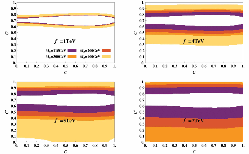
Figure 3: We plot the allowed region of the parameter space ($c$ and $c^{\prime}$) for $f$=1, 4, 5 and 7 TeV, where the four colors correspond to $M_{h}$=115, 200, 300 and 400 GeV, respectively.

Table 1: The allowed regions of the mixing parameter $c^{\prime}$ are presented for $f=1,2$ and $4$ TeV and $M_{h}=115,200,300$ and $400$, respectively. Note that there are two allowed regions for each $f$ and $M_{h}$. Note also that there are common forbidden regions ($0.69<c^{\prime}<0.73$).

Constraints on the mixing parameter $c^{{}^{\prime}}$ and the mass of the heavy gauge boson $B^{{}^{\prime}}$
$f$ value	$M_{h}$	Bottom region	Top region	expected $B^{{}^{\prime}}$ mass
1 TeV	115 GeV	$0.60\sim 0.69$	$0.73\sim 0.80$	$159.4\sim 165.9$,  $159.6\sim 165.9$ GeV
	200 GeV	$0.60\sim 0.67$	$0.75\sim 0.80$	$160.1\sim 165.9$,  $160.5\sim 165.9$ GeV
	300 GeV	$0.59\sim 0.66$	$0.75\sim 0.80$	$160.6\sim 167.1$,  $160.5\sim 165.9$ GeV
	400 GeV	$0.59\sim 0.65$	$0.76\sim 0.81$	$161.2\sim 167.1$,  $161.2\sim 167.6$ GeV
2 TeV	115 GeV	$0.56\sim 0.67$	$0.74\sim 0.82$	$320.1\sim 343.2$,  $319.9\sim 339.3$ GeV
	200 GeV	$0.55\sim 0.63$	$0.78\sim 0.84$	$325.5\sim 346.7$,  $326.2\sim 349.4$ GeV
	300 GeV	$0.53\sim 0.61$	$0.80\sim 0.84$	$329.4\sim 354.3$,  $331.7\sim 349.4$ GeV
	400 GeV	$0.52\sim 0.59$	$0.81\sim 0.85$	$334.3\sim 358.5$,  $335.2\sim 355.6$ GeV
4 TeV	115 GeV	$0.42\sim 0.60$	$0.80\sim 0.90$	$663.4\sim 835.5$,  $637.9\sim 787.5$ GeV
	200 GeV	$0.36\sim 0.53$	$0.85\sim 0.93$	$708.6\sim 948.2$,  $690.0\sim 903.8$ GeV
	300 GeV	$0.32\sim 0.48$	$0.88\sim 0.95$	$756.3\sim 1050.4$,  $739.2\sim 963.4$ GeV
	400 GeV	$0.28\sim 0.44$	$0.90\sim 0.96$	$806.0\sim 1148.7$,  $811.7\sim 1148.7$ GeV

The constraint on $c^{\prime}$ obtained above enables us to estimate the masses of heavy gauge bosons in the LHM. The masses of the heavy gauge bosons $W^{a^{\prime}}_{\mu}$ and $B^{{}^{\prime}}_{\mu}$ are given in terms of mixing parameters by

$$M_{W^{{}^{\prime}}}=\frac{g}{2sc}f~{}\geq gf~{},~{}~{}M_{B^{{}^{\prime}}}=\frac{g^{{}^{\prime}}}{2\sqrt{5}s^{{}^{\prime}}c^{{}^{\prime}}}f~{}\geq\frac{g^{{}^{\prime}}f}{\sqrt{5}}~{}.$$ (43)

In addition to those derived lower bounds on the masses of heavy gauge bosons, we can constrain the size of $M_{B^{{}^{\prime}}}$ further by imposing the constraint on $c^{\prime}$ obtained above.

In Table I, we present the predictions of $M_{B^{{}^{\prime}}}$ for several combinations of $f$ and $M_{h}$ along with the constraints on $c^{\prime}$. As the value of $f$ decreases, $M_{B^{{}^{\prime}}}$ is predicted to get smaller and the theoretical uncertainty gets narrower. In the light of search for new physics, that is a very important implication for the verification of the validity of the LHM when we get to probe or even observe a certain signal for new additional gauge bosons at future colliders.

In conclusion, based on the prediction of $M_{{}_{W}}$ in the LHM, we have compared it with the current and prospective measurements of $M_{{}_{W}}$ and $M_{t}$, and found that the current values and accuracy of $M_{{}_{W}}$ and $M_{t}$ measurements tend to favor the LHM over the SM, although the most recent electroweak data may appear to be consistent with the SM prediction. We have found that the predictions of $M_{{}_{W}}$ in the LHM for $f\gtrsim 26.3$ TeV deviate from the realm of the 1$\sigma$ ellipse for the measurements of $M_{{}_{W}}$ and $M_{t}$, and thus $f=26.3$ TeV can be regarded as the upper bound on $f$. We have discussed how the upper bound on $f$ depends on the Higgs boson mass. As $M_{h}$ decreases, the upper bound on $f$ rapidly increases. We have examined how the parameters $c$ and $c^{\prime}$ can be constrained by comparing the prediction of $M_{{}_{W}}$ with the current precision measurements of $M_{{}_{W}}$ and $M_{t}$. For a given parameter set, it turns out that $c^{\prime}$ is strongly constrained for small $f$ whereas $c$ is not constrained at all. We have studied how the mass of the heavy gauge boson $M_{B^{{}^{\prime}}}$ in the LHM can be extracted from the constraint on $c^{\prime}$ for a given value of $f$. We anticipate that more precision data for $M_{{}_{W}}$ and $M_{t}$ as well as even discovery of the Higgs boson at the LHC would give the LHM even more preference and provide a decisive clue on the evidence of the LHM.

ACKNOWLEDGEMENTS

We thank G. Cvetic for careful reading of the manuscript and his valuable comments. JBP was supported by the Korea Research Foundation Grant funded by the Korean Government (MOEHRD) No. KRF-2005-070-C00030. CSK was supported in part by CHEP-SRC Program and in part by the Korea Research Foundation Grant funded by the Korean Government (MOEHRD) No. KRF-2005-070-C00030. SKK was supported by KRF Grant funded by the Korean Government (MOEHRD) No. KRF-2006-003-C00069.

References

- (1) T. Aaltonen et al. [CDF Collaboration], “First Measurement of the W Boson Mass in Run II of the Tevatron,” Phys. Rev. Lett. 99, 151801 (2007) [arXiv:0707.0085 [hep-ex]].
- (2) T. T. E. Group et al. [CDF Collaboration], “A Combination of CDF and D0 Results on the Mass of the Top Quark,” arXiv:0803.1683 [hep-ex].
- (3) C. Buttar et al., “Les Houches physics at TeV colliders 2005, standard model, QCD, EW, and Higgs working group: Summary report,” arXiv:hep-ph/0604120; R. Boughezal, J. B. Tausk and J. J. van der Bij, “Three-loop electroweak corrections to the W-boson mass and sin**2(theta(lept)(eff)) in the large Higgs mass limit,” Nucl. Phys. B 725, 3 (2005) [arXiv:hep-ph/0504092]; M. Awramik, M. Czakon, A. Freitas and G. Weiglein, “Precise prediction for the W-boson mass in the standard model,” Phys. Rev. D 69, 053006 (2004) [arXiv:hep-ph/0311148].
- (4) J. Erler and P. Langacker, in ”10. Electroweak model and constraints on new physics”, W.-M. Yao et al., J. Phys. G 33, updated version online: http://pdg.lbl.gov/
- (5) R. Barate et al. [LEP Working Group for Higgs boson searches], “Search for the standard model Higgs boson at LEP,” Phys. Lett. B 565, 61 (2003) [arXiv:hep-ex/0306033].
- (6) N. Arkani-Hamed, A. G. Cohen and H. Georgi, “(De)constructing dimensions,” Phys. Rev. Lett. 86, 4757 (2001) [arXiv:hep-th/0104005].
- (7) H. Georgi and A. Pais, “Calculability And Naturalness In Gauge Theories,” Phys. Rev. D 10, 539 (1974); H. Georgi and A. Pais, “Vacuum Symmetry And The Pseudogoldstone Phenomenon,” Phys. Rev. D 12, 508 (1975); N. Arkani-Hamed, A. G. Cohen and H. Georgi, “Electroweak symmetry breaking from dimensional deconstruction,” Phys. Lett. B 513, 232 (2001) [arXiv:hep-ph/0105239].
- (8) N. Arkani-Hamed, A. G. Cohen, E. Katz and A. E. Nelson, “The littlest Higgs,” JHEP 0207, 034 (2002) [arXiv:hep-ph/0206021].
- (9) M. Schmaltz, “The simplest little Higgs,” JHEP 0408, 056 (2004) [arXiv:hep-ph/0407143]; D. E. Kaplan and M. Schmaltz, “The little Higgs from a simple group,” JHEP 0310, 039 (2003) [arXiv:hep-ph/0302049]; H. C. Cheng and I. Low, “TeV symmetry and the little hierarchy problem,” JHEP 0309, 051 (2003) [arXiv:hep-ph/0308199]; H. C. Cheng and I. Low, “Little hierarchy, little Higgses, and a little symmetry,” JHEP 0408, 061 (2004) [arXiv:hep-ph/0405243]; I. Low, “T parity and the littlest Higgs,” JHEP 0410, 067 (2004) [arXiv:hep-ph/0409025]; I. Low, W. Skiba and D. Smith, “Little Higgses from an antisymmetric condensate,” Phys. Rev. D 66, 072001 (2002) [arXiv:hep-ph/0207243].
- (10) C. Csaki, J. Hubisz, G. D. Kribs, P. Meade and J. Terning, “Big corrections from a little Higgs,” Phys. Rev. D 67, 115002 (2003) [arXiv:hep-ph/0211124].
- (11) C. Csaki, J. Hubisz, G. D. Kribs, P. Meade and J. Terning, “Variations of little Higgs models and their electroweak constraints,” Phys. Rev. D 68, 035009 (2003) [arXiv:hep-ph/0303236].
- (12) A. Deandrea, “Little Higgs and precision electroweak tests,” arXiv:hep-ph/0405120; C. Kilic and R. Mahbubani, “Precision electroweak observables in the minimal moose little Higgs model,” JHEP 0407, 013 (2004) [arXiv:hep-ph/0312053]; M. C. Chen, “Models of little Higgs and electroweak precision tests,” Mod. Phys. Lett. A 21, 621 (2006) [arXiv:hep-ph/0601126]; G. Marandella, C. Schappacher and A. Strumia, “Little-Higgs corrections to precision data after LEP2,” Phys. Rev. D 72, 035014 (2005) [arXiv:hep-ph/0502096]; T. Gregoire, D. R. Smith and J. G. Wacker, “What precision electroweak physics says about the SU(6)/Sp(6) little Higgs,” Phys. Rev. D 69, 115008 (2004) [arXiv:hep-ph/0305275]; R. Casalbuoni, A. Deandrea and M. Oertel, “Little Higgs models and precision electroweak data,” JHEP 0402, 032 (2004) [arXiv:hep-ph/0311038].
- (13) J. Alcaraz et al. [LEP Collaborations], “Precision Electroweak Measurements and Constraints on the Standard Model,” arXiv:0712.0929 [hep-ex].
- (14) S. Heinemeyer, W. Hollik, D. Stockinger, A. M. Weber and G. Weiglein, “Testing the MSSM with the mass of the W boson,” arXiv:hep-ph/0611371; see slso, K. Kang and S. K. Kang, “The Minimal supersymmetric standard model and precision of W boson mass and top quark mass,” Mod. Phys. Lett. A 13, 2613 (1998) [arXiv:hep-ph/9708409].
- (15) M. E. Peskin and T. Takeuchi, “Estimation of oblique electroweak corrections,” Phys. Rev. D 46, 381 (1992).
- (16) A. B. Arbuzov et al., “ZFITTER: A semi-analytical program for fermion pair production in e+ e- annihilation, from version 6.21 to version 6.42,” Comput. Phys. Commun. 174, 728 (2006) [arXiv:hep-ph/0507146].
- (17) M. Beneke et al., “Top quark physics,” arXiv:hep-ph/0003033.
- (18) S. Haywood et al., “Electroweak physics,” arXiv:hep-ph/0003275.
- (19) U. Baur, R. Clare, J. Erler, S. Heinemeyer, D. Wackeroth, G. Weiglein and D. R. Wood, “Theoretical and experimental status of the indirect Higgs boson mass determination in the standard model,” [arXiv:hep-ph/0111314].
- (20) T. Abe et al. [American Linear Collider Working Group], “Linear collider physics resource book for Snowmass 2001. 1: Introduction,” in Proc. of the APS/DPF/DPB Summer Study on the Future of Particle Physics (Snowmass 2001) ed. N. Graf, arXiv:hep-ex/0106055.
- (21) B. W. Lee, C. Quigg and H. B. Thacker, “Weak Interactions At Very High-Energies: The Role Of The Higgs Boson Mass,” Phys. Rev. D 16, 1519 (1977).