Scaling Relations for Collision-less Dark Matter Turbulence

Abstract

Many scaling relations are observed for self-gravitating systems in the universe. We explore the consistent understanding of them from a simple principle based on the proposal that the collision-less dark matter fluid terns into a turbulent state, i.e. dark turbulence, after crossing the caustic surface in the non-linear stage. The dark turbulence will not eddy dominant reflecting the collision-less property. After deriving Kolmogorov scaling laws from Navier-Stokes equation by the method similar to the one for Smoluchowski coagulation equation, we apply this to several observations such as the scale-dependent velocity dispersion, mass-luminosity ratio, magnetic fields, and mass-angular momentum relation, power spectrum of density fluctuations. They all point the concordant value for the constant energy flow per mass: $0.3cm^{2}/sec^{3}$, which may be understood as the speed of the hierarchical coalescence process in the cosmic structure formation.

Cosmology: theory, Gravitation, Turbulence, Cosmology: dark matter, Cosmology: observations, Hydrodynamics 98.80.-k 95.35 +d 98.65.-r

I Introduction

Why the stars and galaxies are rotating? What is the origin of the angular momentum? It is known that the planets in our solar system show a remarkable scaling relation between the angular momentum $J$ and the mass $M$ for each planet,

$$J\simeq\alpha\frac{G}{c}M^{2}=\alpha\left({\frac{\hbar}{m_{pl}^{2}}}\right)M^{2},\quad\alpha\simeq 10^{4}$$ (1)

where the unit mass and the angular momentum are measured respectively by the Planck mass $m_{pl}\equiv\left(c\hbar/G\right)^{1/2}=2.18\times 10^{-5}$g and the reduced Planck constant $\hbar\equiv 1.05\times 10^{-27}$erg$\cdot$sec. Only exceptions are the Mercury and the Venus whose rotations are locked with their orbital rotation around the Sun. Although the Sun by itself deviates from the above scaling, the whole solar system is also on this line. Because the relation Eq.(1) holds for the conserved quantities, $J$ and $M$, it strongly suggests some fundamental origin of the planet system.

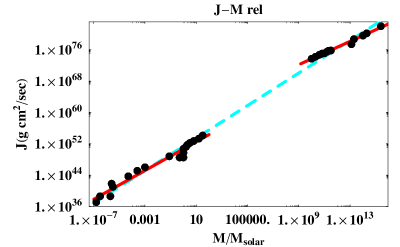
Figure 1: A plot of angular momentum and mass of various astronomical objects. Deta points includes our planets, stars, galaxies, clusters,… [1]. The dashed line represents Eq.(1), or more prcisely $J=1.72\times 10^{-18}M^{2.08}$ in cgs-units. The solid lines represent local scalings for star series and cluster series. Both the local inclinations are slightly smaller than the global one.

Although the extrapolation of the above scaling to the microscopic world actually holds as the Regge trajectory for Hadrons $J\simeq\left(\hbar/\text{Gev}^{2}\right)M^{2}$, it would be more interesting to extrapolate it to much larger scales, such as galaxies and the clusters of them, which actually holds with the same proportionality constant as Eq.(1). This fact is clearly shown by the dashed line in the Figure 1, where the scaling $J\propto M^{2}$ extends over 23-digit [1].

Further examination of this figure reveals the existence of two separate classes of astronomical objects on this scaling line; the star series extending roughly from $10^{-7}M_{\odot}$ to $10^{2}M_{\odot}$, and the cluster series from $10^{10}M_{\odot}$ to $10^{16}M_{\odot}$. Although the whole global scaling looks as $J\propto M^{2}$, the local scaling within each classes is slightly gentle $J\propto M^{1.5}$ to $M^{1.8}$. Since this global scaling extending over 23-digits, if being true, seems to be very difficult to explain from a single mechanism, we concentrate on the local scaling for cluster series in this paper. The objects in this series are primarily characterized by the self-gravity. Thus we now study this scaling relation based on the self-gravity in the expanding universe.

A considerable number of studies have already been made on the origin of angular momentum of galaxies. A typical mechanism of the angular momentum acquisition for galaxies is the tidal torquing (see for example a review paper [2]). Let us consider a relatively dens region in the expanding universe. In general, velocity shear on this region in the Eulerian frame yields a rotation-like motion of this region in the Lagrangian frame. If this dens region actually becomes isolated from the other region by turning around from expanding to contracting due to self-gravity, then this dens region acquires actual angular momentum. However, it is essential for real acquisition of angular momentum that the flow of matter eventually becomes multi-streaming and allows the appearance of vorticity.

The acquired angular momentum

$$\vec{J}=\int_{V}d^{3}x\left(\vec{x}-\vec{x}_{0}\right)\times\vec{v}\left(\vec{x}\right)\rho\left(\vec{x}\right)$$ (2)

is estimated by using Zel’dovich approximation [3] with the Lagrange coordinate $\vec{q}$ as

$$\vec{x}\left({\vec{q},t}\right)=\vec{q}-D\left(t\right)\vec{\nabla}_{\vec{q}}\psi\left(\vec{q}\right)$$ (3)

where $D\left(t\right)$ is the linear growing factor and $\psi\left(\vec{q}\right)$ is the displacement field. Then the angular momentum acquired at the time of turnaround $t_{\text{TA}}$ becomes

$$\vec{J}=-\rho_{0}a\left(t\right)^{5}\int_{V_{\text{com}}}d^{3}q\left(\vec{q}-\vec{q}_{0}\right)\times\dot{D}\left(t\right)\vec{\nabla}\psi\approx t_{\text{TA}}^{1/3}M^{5/3}$$ (4)

where $a\left(t\right)$ is the scale factor, and the integration is taken over the comoving volume $V_{\text{com}}$. The turn-around time $t_{\text{TA}}$ depends on the mass $M$ and the initial condition for the density fluctuations.

This formula of the angular momentum Eq.(4) is numerically checked by the high-resolution galaxy-formation simulation using the P3MSPH code [4]. They have confirmed the power law scaling in Mass $M^{5/3}$ in Eq.(4), but the time dependence $t_{\text{TA}}^{1/3}$ has not been firmly established. According to their calculations, the angular momentum $J$ of each cluster evolves almost linearly in time until the turn-around time $t_{\text{TA}}$, when the most of the full $J$ of the cluster is achieved. Then after the shell crossing time, just after $t_{\text{TA}}$, $J$ fluctuates due to the strong and repeated tidal interactions with neighboring clusters. It is remarkable that the final angular momentum acquired by each cluster still obeys the scaling law in Eq.(4) even after such strong disturbances.

Although the amount of angular momentum is mostly acquired before the turn-around time or the shell crossing time, strongly interacting nonlinear period after that should washout the previous correlations in general. Therefore it would be interesting to examine the dynamics in such nonlinear regime, which may be essential for the establishment of the scaling relations or any correlations which we now observe.

Moreover, within this cluster series, many other scaling relations have been reported, such as the increasing velocity dispersion $\sigma$ with the linear scale $r$, $\sigma^{2}\propto r$. [5], the scaling in average mass-density and the size of the astronomical objects $\rho\propto r^{-1.75}$ [6], power law two-point correlation functions for galaxies $\xi(r)\approx 20\left({r/}\text{{Mpc}}\right)^{-1.8}$ and for clusters of galaxies $\xi(r)\approx 300\left({r/}\text{{Mpc}}\right)^{-1.8}$ [3]. These properties appear to have no relation with the angular momentum especially in the larger scales. Since these properties hold for non-linear structures, it is apparent that we cannot attribute all of the origin of them to the initial conditions. We would like to understand these scaling properties from a simple principle which will hold in the non-linear stage. Is there any basic dynamics which realize all such scaling relations?

For this end, we would like to focus on the turbulent motion of the cold dark matter, i.e. dark turbulence. Since the cold dark matter is collision-less, we cannot apply the standard view of the baryonic turbulence. Actually the collision-less particles cannot form local fluid element which is usually required for fluid description. Thus the dark turbulence is quite different from the ordinary one and even the eddy structure or vector perturbation modes may not dominate. We use the word (dark) turbulence in this sense emphasizing the distinction from the baryonic turbulence. This point will be especially important to understand the difference between our dark turbulence from the old paradigm of the turbulent origin of galaxies. Moreover in our calculations, we never use the eddy picture of turbulence nor assume the vector mode dominance in fluctuations.

The purpose of this paper is to consider all of the above scaling relations from a simple principle. The following is the steps for this purpose. In the next section 2, we explore the possible origin of the scaling in analogy of the fluid turbulence, especially in the form of dark matter, which is not directly rejected from the present observational data. In section 3, we apply the method of Smoluchowski coagulation equation for Navier-Stokes equation and derive the Kolmogorov scaling laws, in appropriate form in use for SGS. In section 4, we explore how extent our proposal can be tested from astronomical observations. In the last section 5, we summarize our study and discuss on further extensions and possible applications of the present discussions.

II Fluid description for self-gravitating systems (SGS) and the dark turbulence

In the present study on the scaling relations, we have restricted our considerations to the cluster series of objects such as globular clusters, galaxies and clusters of galaxies. It is apparent that these structures are mainly governed by the gravity which has no intrinsic scale. However, this fact itself does not determine the scaling index. On the other hand, the virial theorem is expected to hold in the dynamically relaxed systems, and yields a relation between the velocity dispersion $\sigma$, the linear scale $r$ and the mass $M$ as $\sigma^{2}=GM/r$. Recently we have developed an elaboration of this virial theorem and proposed a concept of the local virial relation, which claims that the virial relation holds even a part of a system, which is not necessarily isolated from the rest of the system [7], [8]. However, this virial relation is not enough and yet another relation is necessary to determine the scaling indices. Further, since the above objects are highly non-linear, the linear perturbation method based on the primordial density fluctuations is useless. We directly need to consider highly non-linear regime for our purpose.

We now start our discussion from the reconsideration of the basic fluid description to analyze SGS. Actually there are many common properties between the fluid and SGS. Standard fluid is described by the Navier-Stokes equation for the velocity $\vec{v}\left(\vec{x},t\right)$

$$\frac{\partial\vec{v}}{\partial t}+\left(\vec{v}\cdot\vec{\nabla}\right)\vec{v}=-\frac{\vec{\nabla}p}{\rho}+\nu\Delta\vec{v},$$ (5)

where $p$ is the pressure, $\rho$ is the mass density, and $\nu$ is the friction coefficient. This equation admits the following scaling, with arbitrary real number $\alpha$,

$$r^{\prime} = \lambda^{-1}r,\;\vec{v}^{\prime}=\lambda^{-\alpha/3}\vec{v},\;$$

$$t^{\prime} = \lambda^{-1+\left(\alpha/3\right)}t,\;p^{\prime}/\rho^{\prime}=\lambda^{-2\alpha/3}p/\rho$$ (6)

in the inertial regime, i.e. the dissipative term is negligible compared with the inertial term. Similarly, a set of Jeans equation for SGS and Poisson equation becomes

$$\begin{array}[]{c}\frac{\partial\rho}{\partial t}+\vec{\nabla}\cdot\left(\rho\vec{v}\right)=0,\\ \frac{\partial\vec{v}}{\partial t}+(\vec{v}\cdot\vec{\nabla})\vec{v}+\vec{\nabla}\Phi=0,\\ \vec{\nabla}^{2}\Phi=4\pi G\rho,\end{array}$$ (7)

which also admits the same scaling Eq.(6) supplemented with $\Phi^{\prime}=\lambda^{-2\alpha/3}\Phi,\rho^{\prime}=\lambda^{-\left(2\alpha/3\right)+2}\rho$.

There have been many analytical attempts to reveal the semi-nonlinear regime, just beyond the linear regime. One of them is the Lagrangian method such as the Zel’dovich approximation [3]. This is based on the Lagrangian coordinate $\vec{q}$, which is related to the Eulerian one $\vec{x}$ as Eq.(3), and assumes that the particles develops in the initial potential. Then the mass-density $\rho\left({\vec{x},t}\right)$ is simply given by

$$\rho\left({\vec{x},t}\right)=\rho_{0}\det\left({\delta_{ij}-D\left(t\right)\frac{\partial^{2}\psi}{\partial q_{i}\partial q_{j}}}\right)^{-1}.$$ (8)

This approximation works fairly well to describe the semi-nonlinear evolution until inevitable shell-crossing, or caustic surface, appears when the density $\rho\left({\vec{x},t}\right)$ diverges due to the increase of the linear growth factor ${D\left(t\right)}$. Many authors have tried to avoid or to improve this shortcoming in this approximation. Further, various sophisticated perturbation methods have been proposed to improve the accuracy of approximations but this shell-crossing couldn’t overcome within real values [9]. Actually, shell-crossing is not simply a limitation of the analytic approximations but the initiation of the multi-valued stream, or the appearance of the family of crossing trajectories [10]. It is important to notice that the intrinsic non-linear regime starts from this shell-crossing time, after that the trajectories become chaotic due to the velocity dispersions and the whole system becomes turbulent. Therefore this turbulence should be the clue to solve our problem [11].

At this point, we would like to consider the time scale necessary for the turbulence to become effective. In general in the standard CDM model, smaller the linear scale later the shell-crossing time. Therefore the turbulence is established first at the small scale, say $10^{7}M_{\odot}$, and then the turbulent region gradually extends up to the larger scales of galaxy clusters at redshift of order one. On the other hand, the system acquires most of the angular momentum and kinetic energy which is comparable to the final amount at the time of turn around, as we have already seen in the estimation Eq.(4) and the demonstration by numerical calculations [4]. Just after this turn around time, the flow becomes turbulent at the shell-crossing time. Thus the turbulent velocity field has been already developed at a given redshift corresponds to its shell-crossing time. However, further time period will be necessary for this turbulent flow to become effective and to establish any order such as scaling relations. This period will be estimated later in section 4, using a relevant parameter obtained from the observations.

There have been many studies on the fluid description for SGS in the long history of literature. It is particularly interesting that some authors had already proposed the galaxy formation due to the turbulent motion [12], [13]. However, the matter associated with this turbulent motion was assumed to be baryon, which could easily destroy the observed isotropy of the cosmic background radiation (CMB) and furthermore the turbulent motion would easily decay due to the dissipation through the electromagnetic interactions. Actually the time when this line of study declined overlaps the time when the precision observation on CMB had been developing.

Now the basic understanding on the cosmic matter contents has been drastically changed. The dominant substance is not baryon but some unidentified object which is thought to be collisionless non-relativistic particles. This is often called as dark matter (DM) emphasizing the absence of the interaction with baryons, except gravitational interaction. Therefore what we should consider will be the turbulent motion of DM; thus the title of this paper cosmic dark turbulence (CDT) comes out. Since DM never destroy the isotropy of CMB and never dissipate, the turbulent motion of it seems plausible.

There are several other facts which are crucial for the idea of CDT. (1) Although the vorticity possesses only the decaying mode $\omega\propto t^{-1/3}$ within the linear perturbation theory, it can grow in the non-linear regime [14], [15]. (2) Since the trajectory becomes multi-streaming, the Kelvin’s theorem, which claims the conservation of vorticity along the trajectory in the non-dissipative flow, becomes useless. (3) An analogue of the Reynolds number, i.e. the ratio of the dissipation and the inertial terms, can be calculated in SGS although the system is time-reversible in the microscopic level. An analogue of viscosity may enter the system through the dynamical friction $\nu=O\left(1\right)\ln N\sqrt{rGM}/N$, where $N$ is the total particle number. Then the application of the virial theorem $v^{2}=GM/r$ yields the Reynolds number $R=vr/\nu=O\left(1\right)N/\ln N$, which turns out to be quite large. However, it must be kept in mind that such microscopic friction often becomes irrelevant and is dominated by an effective friction known as eddy viscosity. (4) In general, the stationary turbulence structure is maintained by a steady energy flow, on average, from the large to small scales through the cascade of eddies. This flow is determined by the balance of the energy input at the largest scale and the dissipation at the smallest Kolmogorov scale. In the case of SGS, there are many evidences of hierarchical structure formation in which the coalescence of small clusters successively yield larger clusters. Then the energy flow should exist but the direction may be opposite; from small to large. It is important to notice that the essential properties of the turbulence such as the Kolmogorov laws hold irrespective of the direction of energy flow. Although the above mentioned dynamical friction may not control the flow, the energy flow seems to be essential for the scaling property we consider, irrespective of its direction. This point will be further discussed in the next section. (4) The most important property of CDT is the non-linear interaction among various modes from the smallest to the largest, and the eddy structure is not necessary in our case. This will be well realized in the self gravitating systems.

III Smoluchowski equation and Kolmogorov law

In order to describe the dynamics of coagulation process in general, the mean field approach has been widely used and quite successful. We first consider a simple model in which the whole system is composed from clusters of various masses, which we measure in some arbitrary unit $m_{0}$. Then the variable ${n_{i}}\left(t\right)$ is the number of clusters of mass $i\times m_{0}$ at time $t.$ A typical evolution equation for ${n_{i}}\left(t\right)$, for positive integers $i,j,k$, is given by the Smoluchowski coagulation equation

$$\frac{dn_{i}}{dt}=\frac{1}{2}\sum\limits_{j+k=i}{K_{j,k}n_{j}n_{k}-}n_{i}\sum\limits_{j}{K_{i,j}n_{j},}$$ (9)

where the kernel ${K_{j,k}}$ is the probability that the clusters $j$ and $k$ coalesce into one [16]. Only several exact solutions are known despite its simple appearance [17].

We now consider the scaling transformation

$$i\rightarrow\lambda i$$ (10)

and look for the solution, of Eq.(9), which transforms

$$n_{i}\rightarrow\lambda^{\mu}n_{i}$$ (11)

under the above scaling. We suppose that the kernel has a power law dependence, $K_{i,j}\propto\left({ij}\right)^{\nu/2}$, and also suppose that the mass flow from small to large scales per cluster $\dot{n}_{i}i/n_{i}$ is a constant. Then, since $\dot{n}_{i}$ in Eq.(9) scales as $\dot{n}_{i}\rightarrow\lambda^{\nu+2\mu}\dot{n}_{i}$ (and the time scales as $t\rightarrow\lambda^{-\nu-\mu}t$), we have $1+\nu+\mu=0$. Thus, $\mu=-1-\nu,$ and therefore

$$n_{i}=ci^{-\nu-1},$$ (12)

where $c$ is a mass $i$-independent constant.

It is important to notice that this is not a genuine stationary state since $\dot{n}_{i}$ does not vanish and the configuration $n_{i}$ is always changing. It will be still possible to add an appropriate source term, which is non-zero only for small values of $i$, to maintain the local balance $\dot{n}_{i}=0$ for each cluster $i$, while keeping the same index $-\nu-1$ in Eq.(12). However, as is shown in the above, this index is determined mainly by the actual steady flow and the non-linear kernel ${K_{j,k}}$ which controls it. If we supposed the local balance $\dot{n}_{i}=0$ instead, we would have no robust result which is free from a choice of the source term.

This type of equation Eq. (9) appears in various fields of physics. Actually, the Fourier transform of Eq.(5) becomes

$$\frac{\partial v_{\vec{k}}^{\alpha}}{\partial t}=-ik_{\beta}\sum\limits_{\vec{p}+\vec{q}=\vec{k}}{K_{\vec{k}\mathbf{,}\alpha\gamma}v_{\vec{p}}^{\beta}v_{\vec{q}}^{\gamma}-\nu k}^{2}v_{\vec{k}}^{\alpha}+\text{source term}$$ (13)

where

$${K_{\vec{k}\mathbf{,}\alpha\gamma}=\delta}_{\alpha\gamma}-\frac{k_{\alpha}k_{\gamma}}{k^{2}},$$ (14)

$$v^{\alpha}\left(\overrightarrow{x},t\right){=}\int\frac{d^{3}k}{\left(2\pi\right)^{3}}e^{i\overrightarrow{k}\overrightarrow{x}}v{{}_{\vec{k}}^{\alpha}}\left(t\right){,}$$ (15)

$$\sum\limits_{\vec{p}+\vec{q}=\vec{k}}=\int d^{3}pd^{3}q\delta^{3}\left(\vec{p}+\vec{q}-\vec{k}\right).$$ (16)

The analogy to Eq.(9) is apparent; the Fourier mode $v_{\vec{k}}^{\alpha}\left(t\right)$ replaces the number of clusters $n_{i}\left(t\right)$. Furthermore, the analogy to obtain the power law distribution Eq.(12) is possible.

We consider the scaling transformation

$$\vec{k}\rightarrow\lambda\vec{k}\mathbf{,}\text{ or }\vec{x}\rightarrow\lambda^{-1}\vec{x}$$ (17)

and we look for the solution, for Eq.(13), which transforms

$$v_{\vec{k}}^{\alpha}\rightarrow\lambda^{\mu}v_{\vec{k}}^{\alpha}$$ (18)

under the above scaling. Here we adopt the random phase approximation, in which we progressively take in account the phases of Fourier transformed quantities from lower to higher orders. Therefore, after the inverse-Fourier transformation, they do not simply reproduce the original velocity field in real space, but produce instead statistical variables. We assume the energy flow is a constant $dE\left(\overrightarrow{x}\right)/dt=$ $\varepsilon$, in analogy with the case for Smoluchowski equation. Since the kernel scales as $\left|-ik_{\beta}\sum\limits_{\vec{p}+\vec{q}=\vec{k}}{K_{\vec{k}\mathbf{,}\alpha\gamma}}\right|\rightarrow\lambda^{4}\left|-ik_{\beta}\sum\limits_{\vec{p}+\vec{q}=\vec{k}}{K_{\vec{k}\mathbf{,}\alpha\gamma}}\right|$, we have the scaling

$$\frac{\partial v_{\vec{k}}^{\alpha}}{\partial t}\rightarrow\lambda^{4+2\mu}\frac{\partial v_{\vec{k}}^{\alpha}}{\partial t}$$ (19)

where we consider the inertial regime in which the dissipation and the source terms do not dominate. This scaling suggests that the time should scale as $t\rightarrow\lambda^{-4-\mu}t$ for consistency. Then, since $E\left(\vec{x}\right)=v\left(\vec{x}\right)^{2}/2$, $dE\left(\vec{x}\right)/dt$ scales as

$$dE\left(\vec{x}\right)/dt\rightarrow\lambda^{10+3\mu}dE\left(\vec{x}\right)/dt,$$ (20)

which must be a constant $\varepsilon$. Then we have

$$\mu=-\frac{10}{3}$$ (21)

and , $v^{\alpha}\left(\overrightarrow{x},t\right)$ in Eq.(15) scales as

$$v^{\alpha}\left(\overrightarrow{x}\right)\rightarrow\lambda^{3+\mu}{\ }v^{\alpha}\left(\overrightarrow{x}\right)=\lambda^{-1/3}{\ }v^{\alpha}\left(\overrightarrow{x}\right){\ .}$$ (22)

Therefore, since $\varepsilon\propto$ $\left(v_{\vec{k}}^{\alpha}\right)^{3}$ from Eq.(13), we have

$$v^{\alpha}\left(\vec{x}\right)=\left(\left|\vec{x}\right|\varepsilon\right)^{1/3}f\left(\frac{\vec{x}}{\left|\vec{x}\right|}\right)$$ (23)

where $f$ is a function of only the direction $\overrightarrow{x}/\left|\vec{x}\right|$. As was explained in the above, $v^{\alpha}\left(\vec{x}\right)$ is not simply the original velocity field in real space, but a statistical variable. In other words, the argument $\vec{x}$ in $v^{\alpha}\left(\vec{x}\right)$ does not designate any particular location but only the scale $\left|\vec{x}\right|$ is relevant. Thus $v^{\alpha}\left(\vec{x}\right)$ represents an average velocity difference or the velocity dispersion at the separation $\left|\vec{x}\right|$. Then Eq.(23) corresponds to the Kolmogorov phenomenological theory [18]. In the same way, the energy per mass $E_{k}$ for the Fourier mode $k\equiv\left|\vec{k}\right|$ becomes

$$E_{k} \equiv \int dre^{ikr}E\left(r\right)$$

$$= \int dre^{ikr}v\left(r\right)^{2}/2=O\left(1\right)\Gamma\left(5/3\right)\varepsilon^{2/3}k^{-5/3}$$

where $r\equiv\left|\vec{x}\right|$, i.e.

$$E_{k}=O\left(1\right)\varepsilon^{2/3}k^{-5/3}.$$ (24)

This corresponds to the Kolmogorov 5/3-law which holds in the inertial regime of turbulent fluid. These exponents are quite robust in the inertial regime independent from the spatial dimension, how the energy is dissipated or injected.

Also in this fluid case, the constant energy flow, but not the exact steady state, has been essential to derive these robust results independent from the form of energy supply. The most relevant is the non-linear kernel which drives the constant flow but not simply a local balance between the dissipation and the energy supply from the source term. This point may be confusing in the context of the familiar turbulence in laboratory, which must be supported by steady injection of energy from outside. This laboratory turbulence will be a special case when the Reynolds number is relatively small, say $100-1000$. In the huge system, such as the galaxy whose’ Reynolds number $\approx 10^{10}$, which has wide inertial range, we will be able to check this argument.

In the same spirit as for the Navier-Stokes equation for fluid, we can argue the Fourier transform of Eq.(7) for SGS,

$$\frac{\partial v_{\vec{k}}^{\alpha}}{\partial t}=-ik_{\beta}\sum\limits_{\vec{p}+\vec{q}=\vec{k}}{K_{\vec{k}\mathbf{,}\alpha\gamma}v_{\vec{p}}^{\beta}v_{\vec{q}}^{\gamma}-\nu k}^{2}v_{\vec{k}}^{\alpha}+i\frac{k^{\alpha}}{k^{2}}4\pi G\delta_{\vec{k}}$$ (25)

which is also similar to the Smoluchowski equation, where

$$\delta_{\vec{k}}\left(t\right)=\int d^{3}xe^{i\overrightarrow{k}\overrightarrow{x}}\rho\left(\vec{x},t\right){,}$$ (26)

and $\nu=O\left(1\right)\ln N\sqrt{rGM}/N$. Poisson equation Eq.(7) is used for the above expression for the source term. The continuity equation becomes

$$\dot{\delta}_{\vec{k}}-ik^{\alpha}\sum\limits_{\vec{p}+\vec{q}=\vec{k}}v{{}_{\vec{p}}^{\alpha}\delta_{\vec{q}}=0.}$$ (27)

We now look for the solution, for Eqs.(25, 27), which transforms like Eq.(18). The essential structure of the equations is the same as in the fluid case, except the explicit source term from the density fluctuations $\delta_{\vec{k}}$. We suppose it scales as

$$\delta_{\vec{k}}\rightarrow\lambda^{\nu}\delta_{\vec{k}}$$ (28)

under the scaling transformation Eq.(17). All the exponents are consistently determined as before, in the inertial regime, and we have Eq.(21) and

$$\nu=5+2\mu=-\frac{5}{3}.$$ (29)

Thus the Kolmogorov laws Eqs.(23)-(24) still hold in the inertial regime.

In the case of collision-less SGS, the dissipation due to the binary collision nor the external driving force are not thought to control the steady energy flow. However in case of the cold dark matter, we naturally expect a hierarchical coalescence process to form structures. Since smaller clusters coalesce to form a larger cluster, the energy flows from small scale to large scale in real space. This is more like the process described by Smoluchowski coalescence equation. Although the flow direction is opposite to the case of fluid turbulence, in which the energy flows from large to small, the existence of a steady energy flow is essential to derive Kolmogorov scaling relations. Thus we could obtain the same Kolmogorov laws in SGS. It is also important in the above calculations that we never used the eddy structure. This demonstrates our claim that the CDT does not require eddies or vector mode dominance.

The above Kolmogorov equations provide us a new relation which is essential to solve our problem. The velocity difference at the scale $\left|\overrightarrow{x}\right|:v^{\alpha}\left(\overrightarrow{x}\right)$ in Eq.(23) is a statistical variable which can also be understood as the velocity dispersion $\sigma_{r}$ at the scale $r=\left|\overrightarrow{x}\right|$. Therefore our first relation is

$$\sigma_{r}=\left(r\varepsilon\right)^{1/3},$$ (30)

which claims that the velocity dispersion increases with the scale. A numerical factor of $O\left(1\right)$ on the right hand side of Eq.(23) is absorbed into the parameter $\varepsilon$. By utilizing the local virial relation with this equation, we have the mass at the scale $r$ as

$$M_{r}=\frac{r\sigma_{r}^{2}}{G}=\frac{\varepsilon^{2/3}}{G}r^{5/3},$$ (31)

or equivalently, the mass density at the scale $r$ as

$$\rho_{r}=\frac{M_{r}}{\left(4\pi/3\right)r^{3}}=\frac{\varepsilon^{2/3}}{\left(4\pi/3\right)G}r^{-4/3},$$ (32)

which claims that the mass density reduces with the scale. This is fully consistent with Eqs.(29, 28 and 26), as should be. We now examine possible observational tests on the above results in the next section.

IV Observational tests

We now examine the scaling relations Eqs.(30)-(32), which we obtained in the previous section, by applying them to the observational data recently available. Certainly our discussion based on the autonomous dynamics of CDT will be limited both from upper and lower scales. The upper boundary comes from the fact that the larger scale structures are better described by the deterministic evolution which is often analyzed by linear approximations. The lower boundary comes from the fact that the smaller scale structures have nothing to do with the dark matter turbulence nor hierarchical coalescence processes but may be better described by the baryonic interactions or the hierarchical decay processes. We should be careful for such applicability range in the following tests. A single parameter $\varepsilon$, the steady energy flow per particle, in our argument on CDT, will be found below.

IV.1 Scale dependent velocity dispersion

We first apply Eq.(30) for observations for galaxies and clusters. The line-of-sight velocity dispersion for various astronomical objects as a function of the linear scale is shown in the Figure 2. The data points are from Sanders & McGaugh [5], and represents, from large to small scales, X-ray emitting clusters of galaxies, massive elliptical galaxies, dwarf spheroidal satellites of the Galaxy, compact elliptical galaxies, massive molecular clouds in the Galaxy, and globular clusters. Among them, dwarf spheroidal satellites and molecular clouds (marked as filled triangles) are irrelevant for our argument. This is because the extended dwarf spheroidal satellites of the Galaxy are located near to the dominant Galaxy, and therefore any systematic tidal effects cannot be avoided [19]. On the other hand, because the massive molecular clouds in the Galaxy are located very inside the galaxy disk, any dynamical contamination cannot be avoided [20].

On top of the observational data, disregarding the above mentioned irrelevant species, a solid line is drawn which represents Eq.(30) with $\varepsilon=0.3[$cm${}^{2}/\sec^{3}]$. This value will be fixed throughout this paper. It is apparent from the graph that the larger-scale structure has higher velocity dispersion. It is important to notice that this scaling law only holds globally in the whole scale region, from $1pc$ to $1Mpc$, but not locally within the individual species of objects. For example, we cannot claim the scaling only from the data for galaxies because of huge scatter. The above value for the parameter $\varepsilon$ allows error of factor two when we consider the global fitting.

This value $\varepsilon=0.3[$cm${}^{2}/\sec^{3}]$ also determines the intrinsic upper limit of the size for the applicability of our argument. The energy of an object of size $r$ is roughly given by $\sigma^{2}=\left(\varepsilon r\right)^{2/3}$ per mass, from Eq.(30), which should be accumulated by the steady energy flow during the time span $T$ as $\varepsilon T$. Equating them $r=\varepsilon^{1/2}T^{3/2}$ and putting the cosmic age for $T$, we have $r\approx 50Mpc$, which yields the intrinsic upper limit in size. Another estimation is also possible if we temporary assume the eddy picture of turbulence. A necessary time for an eddy of size $r$ to make one revolution is $T=2\pi r/v$ with Eq.(30). Requiring that this should not exceed the cosmic age for the effective relaxation, makes the upper limit as $r=\left(2\pi\right)^{-3/2}\varepsilon^{1/2}\left(\cos\text{mic age}\right)^{3/2}\approx$ $3.2Mpc$. Thus we roughly understand that our discussion cannot be applied beyond these scales.

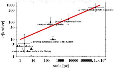
Figure 2: The line-of-sight velocity dispersion for various astronomical objects as a function of the linear scale. The deta points are from Sanders & McGaugh [5], and represents, from large scale to small scale, X-ray emitting clusters of galaxies, massive elliptical galaxies, dwarf spheroidal satellites of the Galaxy, compact elliptical galaxies, massive molecular clouds in the Galaxy, and globular clusters. The solid line representing Eq.(30) is drawn disregarding the data of satellites and molecular clouds (marked as filled triangles) since they might be dynamically contaminated from our Galaxy or from the Galactic disk.

IV.2 Mass-Luminosity ratio

We now examine the mass density as a function of size. From Eq.(32), we have

$$\rho_{DM}=\frac{\varepsilon^{2/3}}{\left(4\pi/3\right)G}r^{-4/3},$$ (33)

for dark matter. On the other hand, many observations indicate that the luminous matter behaves differently,

$$\rho_{LM}=\rho_{LM0}r^{-1.8}$$ (34)

where $\rho_{LM0}$ is some constant. Combining these equations of different nature, the ratio of the gravitational mass and luminous mass becomes

$$M/L\equiv\frac{\rho_{DM}+\rho_{LM}}{\rho_{LM}}\propto r^{0.48},$$ (35)

which claims that the ratio $M/L$ increases with scale. This is compared with observations of Bahcall et al. [21]. The solid line in Figure 3 represents Eq.(35), with $\varepsilon=0.3[$cm${}^{2}/\sec^{3}]$, which is always fixed in this paper, and $\ \rho_{LM}/\rho_{DM}=6\times 10^{-4}$ at $r=1$AU. The latter parameter is just for a calibration and is not at all any prediction of $\rho_{LM}/\rho_{DM}$ at $1AU$, since the DM turbulence cannot affect the physics at $1AU$. Allowing large scatter, the solid line traces the overall tendency of the data up to about $10Mpc$, beyond this scale there seems to be a systematic saturation of the ratio. We must notice that CDT only predicts Eq.(33) for DM, but Eq.(34) is a result of observations.

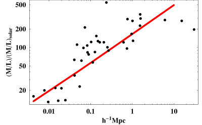
Figure 3: Mass-Luminosity ratio in various scales. The points represent various astronomical objects [21]. The solid line represents Eq.(35) with $\varepsilon=0.3[$cm${}^{2}/\sec^{3}]$ and $\ \rho_{LM}/\rho_{DM}=6\times 10^{-4}$ at $r=1$AU.

IV.3 Mass-angular momentum relation

We now study the angular momentum-mass relation, which has been our original motivation of the present study. By utilizing the rigid body approximation, virial relation, and Eq.(31), we have the expression

$$\frac{J}{M^{2}}=\frac{2}{5}G^{4/5}\varepsilon^{-1/5}M^{-1/5}$$ (36)

with $\varepsilon=0.3$ as before. It is worth mentioning that this mass dependence of the angular momentum $J\propto M^{9/5}$ is very similar to the one predicted from the tidal torquing Eq.(4) $J\propto M^{5/3}$. A mild dependence on $M$ in the factor $t_{\text{TA}}^{1/3}$ in Eq.(4) even works to reduce the difference of them. We would like to emphasize that the latter is the angular momentum acquired by the turn around time and the former is one regulated by turbulence later.

This result, expressed as the solid line in Figure 4, is compared with observations; simple points are from Muradian et al. [1], and points with error bar are from Brosche [22]; Brosche & Tassie [23]. It should be noticed that the vertical axis $J/M^{2}$ extends over 2-digit, while the horizontal axis $M$ extends over 20-digit. Within this extension, the range of our consideration is only the right half of this graph for cluster series.  Although the data have huge scatter, the relation Eq.(36) is not excluded. It is also noticed that in the left half of this graph, a similar line with the same inclination can fit the rest of the data which includes planets and stars. Let us have discussion on this fact in the summary section.

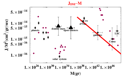
Figure 4: The relation between $J/M^{2}$ and $M$ for various objects; simple points are from Muradian et al. [1], and points with error bars are from Brosche [22]; Brosche et al. [23]. Double stars and the open clusters, marked by triangles, are not considered to be SGS and thus excluded from our discussion. The solid line represents our relation Eq.(36) with $\varepsilon=0.3$.

IV.4 Power spectrum of density fluctuations $P\left(k\right)$

The power spectrum of the density fluctuations $P\left(k\right)$ can be expressed in terms of the two-point correlation function $\xi\left(r\right)$ as

$$P\left(k\right)=4\pi\int_{0}^{\infty}r^{2}dr\frac{\sin\left(kr\right)}{kr}\xi\left(r\right),$$ (37)

in which $\xi\left(r\right)$ can be expressed by the density function $\rho\left(r\right)$ which is already obtained as Eq.(32) for DM. Thus, we have

$$\xi\left(r\right)=\frac{\rho\left(r\right)}{\rho_{0}}=\xi_{0}r^{-4/3},$$ (38)

where $\xi_{0}=$ $\varepsilon^{2/3}/\left(4\pi G\rho_{0}/3\right)$, and

$$P\left(k\right)=2\sqrt{3}\pi\Gamma\left(\frac{2}{3}\right)\xi_{0}k^{-5/3}.$$ (39)

This relation for DM is expressed as the dashed line in Figure 5, with the appropriate parameter $\rho_{0}$ for normalization so that it matches to WMAP data $\sigma_{8}=0.8$ [24]. Immediate caution must be mentioned here. The scale range shown in Fig.(5) is linear to quasi-linear regime($0.02<k\left(\text{hMpc}^{-1}\right)<0.5$). The linear regime is outside of the applicability of our turbulence model, and the quasi-linear regime is marginal. Therefore the dashed line in the figure should be understood as an asymptotic extrapolation from the non-linear region ($0.5<k\left(\text{hMpc}^{-1}\right)$) where CDT model can describe. Although an applicability of our model is limited, this regime is important in the sense that the bias, the ratio of the density fluctuations of DM and luminous matter, becomes very simple and is almost a constant in this regime. Therefore luminous matter power spectrum obtained from direct observations faithfully traces DM power spectrum predicted from our CDT model. Keeping these facts and restrictions in mind, it would be interesting to compare our results with observations.

The above predictions from CDT model is compared with the recent observational data of 2dF and SDSS(DR5) [25], which are drawn, respectively, by dots and squares. The agreement of the slope for the non-linear region $k>0.07$ should not be taken seriously as was explained in the above; our CDT model cannot explain the power spectrum in this regime. On the other hand, other type of observations is often approximately expressed by an analytic form [26],

$$P_{\text{obs}}\left(k\right)=\frac{2\pi^{2}}{k^{3}}\frac{(k/k_{0})^{1.6}}{1+(k/k_{c})^{-2.4}}.$$ (40)

This is shown as gray shade in Figure 5, with the parameter $k_{0}=0.19(h^{-1}$Mpc$)^{-1}$, and $k_{c}=0.015-0.025(h^{-1}$Mpc$)^{-1}$.

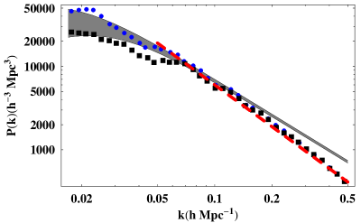
Figure 5: The power spectrum of density fluctuations. The points and squares represent the data from 2dF and SDSS(DR5), respectively [25]. The shaded region represents the average of the other type of observations [26]. The dashed line is our result Eq.(39) with the normalization $\sigma_{8}=0.8$ suggested from WMAP data [24]. This dashed line is an asymptotic extrapolation of the non-linear regime, where our CDT model is justified, and the partial agreement with 2dF/SDSS(DR5) results should not be taked seriously. The CDT model cannot describe this linear to quasi-linear regime with sufficient confidence.

IV.5 Scale dependent Magnetic field

Now we consider a possible relation between our arguments on CDT and the large scale distribution of cosmic magnetic fields. Actually, the magnetic field $\vec{B}$ and the vorticity $\vec{\omega}\equiv rot\vec{v}$ follow the very similar equations of motion and a rough argument based on this fact is found in the book by Landau & Lifshits [27], section 74. Generation of the cosmic magnetic field is studied in Ref. [28], and further development of the magnetic field is discussed in Ref. [29], for example. Magnetic fields in the higher redshift is discussed in Ref. [30-31].

Although a large number of studies have been made on cosmic magnetic fields, little is known about the generation and development of them on all scales. Thus we simply assume here the following conditions as a starting point for discussions.

1. The dynamo mechanism is a universal process to convert the kinetic energy into magnetic fields in various cosmic scales.

2. Baryons should faithfully follow the motion of DM at least at later stage of the universe.

3. The conversion rate $\Gamma$ is a constant in all scales.

Immediate explanations for them are necessary. The assumption 1 is not at all verified at present. However if the turbulence is the essence to develop and regulate the magnetic field, and the similarity in the equations for $\vec{B}$ and $\vec{\omega}$ were true, then such model can be workable. The assumption 2 may sound strange, because one usually imagine that DM cannot interact with baryons, it simply form a static potential well, in which baryons fall straightly. However, since DM is moving according to Eq.(30), with velocity dispersion, its potential well may not be “static”. Furthermore in the study of angular momentum of galaxies, there is empirical relation that the DM has the same specific angular momentum as that for baryons [32]. We have good grounds for thinking that the baryons are dynamically coupled to turbulent motions of DM, because the empirical relation is widely supported. The assumption 3 is total ad hoc; we would like to consider the deviation of the scaling in the magnetic field, if any, is partially due to the variation of this conversion rate.

If we adopt the above conditions,then the resultant magnetic field should have a systematic scale dependence which reflects the scale dependent kinetic energy in the turbulence. The kinetic energy at the scale $r$ becomes

$$\frac{1}{2}\rho_{DM}\left\langle{v^{2}}\right\rangle=\frac{3}{8\pi G}\varepsilon^{4/3}r^{-2/3}.$$ (41)

Then, since the portion of $\Gamma$ of this quantity is supposed to tern into the energy density of the magnetic field $\vec{B}^{2}/\left(8\pi\right)$, we can estimate the magnetic field produced from the dynamo mechanism as

$$\vec{B}_{estimated}=\left(\frac{3\Gamma}{G}\right)^{1/2}\varepsilon^{2/3}r^{-1/3}.$$ (42)

On the other hand, the strength of the magnetic field $B$ obtained from cosmological observations in various scales are depicted in Figure 6 [33], [34]. Guided these data, we have chosen the value $\Gamma=0.02$, which means that the energy of the magnetic field is 12 percent of the kinetic energy in the baryonic form. The estimated magnetic field Eq. (42) from CDT, with this $\Gamma$, is depicted in Figure 6 by the solid line. Reflecting the above bold assumptions, the fit is not so remarkable though general tendency is not excluded from observations. Furthermore the magnetic fields seem to form steeper slope at smaller scale than about parsec, which coincides with the smallest scale of the cluster series, only beyond that we can apply the argument of CDT.

For the larger scales beyond about $10$ Mpc, the dynamical time becomes larger than the Hubble time, where we cannot apply our argument.

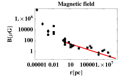
Figure 6: Cosmic magnetic fields in various scales. The deta are from Ref. [33], marked by stars and Ref. [34], marked by squares and diamonds. The solid line represents Eq.(42) with parameter $\Gamma=0.02$. This fit is violated below the distance about the parsec scale, and another power seems to develope below there.

V Summary and Discussions

We summarize our study and discuss on further extension and possible applications of it. We started our study from an interesting scaling law $J\propto M^{2}$ which holds for angular momentum $J$ and the mass $M$ of astronomical objects from the scale of planets toward that of clusters of galaxies. Focussing on the cluster series, such as globular clusters, galaxies and clusters of galaxies, we extracted the nature of the fully non-linear stage of dark matter, after the formation of caustic surface, in analogy between SGS and the fluid turbulence. The essential Kolmogorov laws were rederived from the Fourier transformed Navier-Stokes equation and equations for SGS, by demanding the existence of a steady energy flow characterized by a single parameter $\varepsilon$. This is an analogue of the case of Smoluchowski coagulation equation, which admits scaling solution by demanding the steady mass flow. Then we tried to test our considerations in several cosmological observations, such as the velocity dispersion, Mass-Luminosity ratio, $J-M$ relation, Power spectrum of density fluctuations, and the cosmic magnetic fields. They all point the concordant value for the constant energy flow per mass: $\varepsilon=0.3$cm${}^{2}/$sec³.

Finally we would like to point out several issues on which we should address in our subsequent studies for CDT.

1. We would like to evaluate the energy flow $\varepsilon$ for DM, which may be associated with the hierarchical coalescence process in which smaller clusters continuously form larger clusters. This process provides the bottom-up scenario for the formation of large scale structure especially in the cold DM model. We would like to check whether the value we used $\varepsilon\approx 0.3[$cm${}^{2}/\sec^{3}]$ is consistent with the hierarchical coalescence evolution of DM. Roughly estimated, this accumulation rate of kinetic energy yields a galaxy within about $10^{8}$ years.

2. If the above is the case for DM, then we would like to apply the same analysis to our planet system, which is also considered to have the coalescence evolution as its origin [35]. Actually in the left half of Figure 3, the planet and star systems seem to admit the fitting line with the same slope $-1/5$ as the case for DM but with larger parameter value for $\varepsilon$. It turns out that the appropriate value for $\varepsilon$ becomes of order $10^{15}$, which seems to be too large to be explained from a simple coalescence process as in the case for DM. Some violent mechanism, which allow huge energy transfer rate or catastrophic coalescence, is expected in the case for planet formation process.

3. In the fluid turbulence, there holds another relation often called Kolmogorov 4/5 law

   $$\left\langle\left(\delta v\left(\vec{r}\right)\right)^{3}\right\rangle=-\frac{4}{5}\varepsilon r,$$ (43)

   which is essential to explain the energy flow takes place from low frequency modes to high frequency modes on average. Then what is the analogous relation for SGS and how is it relevant in the universe? Although we do not know the answer, it will be important to notice the fact that SGS [36] shares some common properties with the fluid turbulence [37], such as the negative skewness and the exponential distribution function of the velocity-difference, etc. These common properties will be a good starting point for further discussion.

4. It would be interesting if we could actually transform Eq.(25) into the Smoluchowski form like Eq.(9) which directly expresses the coalescence evolution of SGS. If this is the case, the possible scaling solution, which may asymptotically realize, may correspond to the Schechter function [3] which has a typical form,

   $$\phi\left(L\right)dL=\eta_{\ast}\left(\frac{L}{L_{\ast}}\right)^{-1.25}\exp\left(-\frac{L}{L_{\ast}}\right)\frac{dL}{L_{\ast}},$$ (44)

   where $\phi\left(L\right)dL$ represents the frequency of the object of luminosity $L$. If the cosmological objects are formed after many coalescence processes, then the Smoluchowski equation will be more appropriate than the Press-Schechter theory [3], in which a single collapse determines the population of objects at the corresponding scale. If this is the case, the index $\alpha$ for the kernel ${K_{\mathbf{k,}\alpha\gamma}}$ (see just below Eq.(9)) should be about $-1.25-\left(-1\right)=0.25$. The exponential factor $\exp\left(-\frac{L}{L_{\ast}}\right)$ seems to be a natural tail of the distribution which is gradually evolving without runaway coalescence.

5. We could not complete the argument on the velocity-luminosity (or mass) relation [38] which holds within a single species of object, from our point of view. If we simply apply our argument for luminous objects, we would have, from $\rho_{LM}=\rho_{LM0}r^{-1.8}$, the luminosity

   $$L=\left(\frac{L_{\ast}}{M_{\ast}}\right)\frac{4\pi}{3}\rho_{LM0}\varepsilon^{-1.2}v^{3.6}$$ (45)

   as a function of the velocity $v$ or the velocity dispersion $\sigma$ at that scale, provided appropriate reference ratio $L_{\ast}/M_{\ast}$ is given. For DM, we have, from $\rho_{DM}=\rho_{DM0}r^{-4/3}$, the mass expression

   $$M=\frac{4\pi}{3}\rho_{DM0}\varepsilon^{-5/3}v^{5}.$$ (46)

   On the other hand, several tight relations are obtained for each type of galaxies. For spiral galaxies, Tally-Fisher relation of the form Eq.(45) holds with the variation of index from 3 for B-band to 4 for K band observations. For elliptical galaxies, a tight relation on the fundamental plane is established, $r=$const.$\sigma^{1.24}I^{-0.82}$ where $I=L/\left(2\pi r^{2}\right)$ is the average surface brightness. Although we can simply apply our argument to yield

   $$r^{1.07}=\text{const.}\sigma^{1.24}I^{-0.82},$$ (47)

   which is almost consistent with the above, we cannot obtain the relation in the form of a plain among three independent parameters; all quantities are functions of only $r$ in our case.

We would like to elaborate our argument along the above issues and hope we can report the results soon.

Acknowledgements

The authors would like to thank Osamu Hashimoto, Hidenori Takahashi for relevant discussions on the turbulence, Osamu Iguchi, Yasuhide Sota, and Tohru Tashiro for discussion on the local virial relation, Nozomi Mori for the cosmic magnetic fields and dynamo theory, Masaaki Morita, Hideaki Mouri for turbulence and fate of cosmic vorticity, Kiyotaka Tanikawa for showing us his paper before publication and providing us relevant references on $J-M$ relation, Takayuki Tatekawa for higher-order density perturbation theories. All of their help has been crucial for the completion of this paper.

References

- (1) R. Muradian, S. Carneiro, & R. Marques, Apeiron 6, 186 (1999).
- (2) B. M. Schaefer, arXiv:astro-ph/0808.0203v1 (2008).
- (3) P. J. E. Peebles, Principles of Physical Cosmology (Princeton Series in Physics), Princeton Univ. Press (1993).
- (4) B. Sugerman, F. J. Summers, M. Kamionkowski, MNRAS 311, 762 (2000).
- (5) R. H. Sanders, & S. S. McGaugh, Ann. Rev. Astron. Astrophys. 40, 263 (2002). [arXiv:astro-ph/0204521]
- (6) G. Vaucouleurs, de, Science 167, 1203 (1970).
- (7) O. Iguchi, Y. Sota, A. Nakamichi, & M. Morikawa, Phys. Rev. E 73, 046112 (2006); O. Iguchi, Y. Sota, T. Tatekawa, A. Nakamichi, & M. Morikawa, Phys. Rev. E 71, 016102 (2004); Y. Sota, O. Iguchi, M. Morikawa, & A. Nakamichi, Prog. Theor. Phys. Suppl. 162, 62 (2005).
- (8) Y. Sota, O. Iguchi, T. Tashiro, & M. Morikawa, arXiv:astr-ph/009.245v1 (2007).
- (9) G. Yoneda, H. Shinkai, & A. Nakamichi, Phys Rev. D 56, 2086 (1997).
- (10) T. Buchert, arXiv:astro-ph/9901002v2 (1999).
- (11) M. Morikawa, AIP conference proceedings Dynamics and Thermodynamics of systems with long-range interactions, ed by A. Campa, et. al., 269 (2007).
- (12) C. F. von Weizsacher, Naturwiss. 35, 188 (1948).
- (13) G. Gamow, Phys. Rev. 86, 251 (1952).
- (14) M. Sasaki & M. Kasai, arXiv:astro-ph/9711252v1 (1997).
- (15) R. Scoccimarro, arXiv:astro-ph/0008277v1 (2000).
- (16) M. v. Smoluchowski, Phys. Z. 557, 585 (1916).
- (17) C. Hayashi & Y. Nakagawa, Prog. Theor. Phys. 54, 93 (1975).
- (18) A. N. Kolmogorov, Dokl. Akad. Nauk SSSR 30, 9 (1941).
- (19) M. Mateo, Annu. Rev. Astron. Astrophys. 36, 435 (1998).
- (20) P. M. Solomon, A. R. Rivolo, J. Barrett & A. Yahil, ApJ 319, 730-741 (1987).
- (21) N. A. Bahcall, R. Cen, R. Dav, J. P. Ostriker & Q. Yu, ApJ 541, 1 (2000).
- (22) P. Brosche, Comments Asrophys. 11-5, 213 (1986).
- (23) P. Brosche & L. J. Tassie, A&A 219, 13 (1989).
- (24) G. Hinshaw, J. L. Weiland, R. S. Hill, N. Odegard, et.al. arXiv:astro-ph/0803.0732v1 (2008).
- (25) A. G. Sanchez & S. Cole, arXiv:astro-ph/0708.1517v2 (2007).
- (26) P. Coles, F. Lucchin, Cosmology: The Origin and Evolution of Cosmic Structure, John Wiley & Sons Inc (2002).
- (27) L. D. Landau, E. M. Lifshits & L. P. Pitaevskii, Electrodynamics of Continuous Media (Course of Theoretical Physics) Butterworth-Heinemann Oxford, 2nd ed. (1984).
- (28) N. Y. Gnedin, A. Ferrara & E. G. Zweibel, ApJ 539, 505 (2000).
- (29) A. A. Schekochihin, S. C. Cowley, R. M. Kulsrud, G. W. Hammett & P. Sharma, ApJ 629, 139 (2005).
- (30) P. P. Kronberg, Magnetic Fields in Galaxy Systems, Clusters and Beyond, Lect. Notes Phys. 664, 9 (2005).
- (31) P. P. Kronberg, M. L. Bernet, F. Miniati, S. J. Lilly, M. B. Short, D. M. Higdon, ApJ (in press), arXiv:astro-ph/0712.0435v1 (2007).
- (32) C. Tonini & P. Salucci, ApJ 638, L13 (2006).
- (33) J. P. Vallee, ApJ 360, 1 (1990).
- (34) J. P. Vallee, Astrophysics and Space Science 234, 1 (1995).
- (35) E. Kokubo & S. Ida, Icurus 123, 180 (1996); , Icarus 131, 171 (1999); Icarus 143, 15 (2000).
- (36) A. Yoshisato, M. Morikawa & H. Mouri, MNRAS 343, 1038 (2003).
- (37) B. Chabaud, A. Naert, J. Peinke, F. Chilla, B. Castaing & B. Hebral, Phys. Rev. Lett. 73, 3227 (1994).
- (38) J. Binney, S. Tremaine, Galactic Dynamics (Princeton Series in Astrophysics), Princeton Univ. Press (2008).