GH$\alpha$FaS: Galaxy H-alpha Fabry-Perot System for the WHT

Abstract

GH$\alpha$FaS  a new Fabry-Perot system, is now available at the William Herschel Telescope. It was mounted, for the first time, at the Nasmyth focus of the 4.2 meter WHT on La Palma in July 2007. Using modern technology, with a spectral resolution of the order R$\sim$15000 , and with a seeing limited spatial resolution, GH$\alpha$FaS will provide a new look at the H$\alpha$-emitting gas over a 4.8 arcminutes circular field in the nearby universe. Many science programs can be done on a 4.2 metre class telescope in world class seeing conditions with a scanning Fabry-Perot. Not only galaxies but HII regions, planetary nebulae, supernova remnants and the diffuse interstellar medium are subjects for which unique data can be aquired rapidly. Astronomers from the Laboratoire d’Astrophysique Expérimentale (LAE) in Montréal, the Laboratoire d’Astrophysique de Marseille (LAM-OAMP), and the Instituto de Astrofísica de Canarias (IAC), have inaugurated GH$\alpha$FaS by studying in detail the dynamics of some nearby spiral galaxies. A robust set of state-of-the-arts tools for reducing and analyzing the data cubes obtained with GH$\alpha$FaS has also been developed.

1 Introduction

From 2007 July 2nd to July 8th, the new private instrument GH$\alpha$FaS  was commissioned on the Whilliam Herschel Teslecope (WHT). The acronym GH$\alpha$FaS  stands for Galaxy Halpha Fabry-Perot (FP) System, and gives an idea of the nature and the prime use of the instrument. It is a new generation FP interferometer, whose chief and powerful advantage is its high sensitivity photon counting detector coupled to a large field of view. GH$\alpha$FaS  (which sounds like the Spanish word, ”gafas”, for a pair of glasses) is used on the GHRIL platform of the Nasmyth focus of the WHT.

GH$\alpha$FaS  is an improved version of the scanning Fabry-Perot system FaNTOmM (Hernandez et al., 2003), which is a resident instrument at the Observatoire du mont Mégantic (OmM) 1.6 m telescope and which has also been used as a visitor instrument on the Canada-France-Hawaii (CFH) and ESO La Silla 3.6 m telescopes. The complete system is composed of a focal reducer, a calibration unit, a filter wheel for the order sorter filters, an FP etalon and a photon-counting (IPCS) camera. The IPCS is composed of an Hamamatsu intensifier multi-channel plates (MCP) tube which intensifies every generated electron coming from the photocatode by a factor 10⁷. Each photon event, recorded on a DALSA CCD, is then analyzed by a centering algorithm. With this amplification, the camera has essentially no readout noise. Because of this, a zero noise IPCS is to be preferred to CCDs at very low flux level (Gach et al., 2002), even if the GaAs IPCS has only a DQE of $\sim$26%. Moreover, because of the fast scanning capability, it can average out the variation of atmospheric transmission which is not possible with the long integration times needed per channel for the CCDs in order to beat the read-out noise.

In the last 3 years, around 150 galaxies were observed with the FaNTOmM system on the OMM, CFH and ESO La Silla telescopes in the context of 3 large surveys: the SINGS samples (Daigle et al. 2006 & Dicaire et al. 2007), a survey of barred galaxies, the BH$\alpha$BAR  sample (Hernandez et al. 2005) and a sample of Virgo spirals (Chemin et al. 2006). While the first scientific justification was to derive high spatial resolution optical rotation curves for mass modeling purposes, the data was also used by IAC astronomers to constrain the role of gravitational perturbations as well as feedback from individual HII regions on the evolution of structures in galaxies (Fathi et al., 2007; Relaño et al., 2007) and by a Berkeley-Munich group, the GÉPI group at Observatoire de Paris and Laboratoire d’Astrophysique de Marseille (LAM) to compare those local samples to high z galaxies.

GH$\alpha$FaS comes with its own custom designed focal reducer developed to be optically and mechanically compatible with the Nasmyth focus of the WHT. The system has its own control and data acquisition system. It has a 4 arcmin circular field with a 0.4 arcsec pixel and a minimum of $\sim$5 km/s velocity resolution. Full acquisition and reduction software (mainly based on IDL routines) is provided by the Montréal and IAC groups. The project will be done in 3 phases. For Phase I (July 2007), the optical system (focal reducer, filter wheel & calibration unit) has been delivered to the WHT and used with the Marseilles IPCS camera for this first run. For Phase II (beginning of 2008), an improved GaAs IPCS will be added to the system. Phase III (mid 2008) will provide an FP controller to replace the old CS100 technology (provided by IC Optical formerly Queen’s Gate) and possibly a Tunable Source to calibrate the data at the observing wavelength.

GH$\alpha$FaS is presented in this paper. Section 2 describes the science cases for the GH$\alpha$FaS instrument, while Section 3 discusses the technical details of the instrument. In Section 4, the data preparation and reduction procedures are presented while a sample of the first results is shown. The conclusions are given in Section 5.

2 GH$\alpha$FaS Science Drivers

Several instruments exist that provide two dimensional maps for kinematical and population analysis of galaxies or other astronomical objects. Those observations are mainly based on two different techniques of wavelength separation: dispersive or scanning. The former uses fibers (Virus: Hill et al. 2006, Argus: Kaufer et al.2003, Integral: Arribas et al. 1998), micro-lenses (first concept done by Courtes (1982), Tiger: Bacon et al. 1995, Sauron Bacon et al. 2001), image slicers (SINFONI: Eisenhauer et al. 2003, MUSE: Henault et al. 2004, WiFes: Dopita et al. 2007, SWIFT: Thatte et al. 2006, FRIDA: López et al. 2006, and references therein) and the later Fabry-Perot etalons in a pupil (FaNTOmM in Hernandez et al. 2003, Cigale: Boulesteix et al. 1984, (HIFI): Bland et al. 1990, Taurus: Atherton et al. 1982. GH$\alpha$FaS  is a scanning instrument with the largest field-of-view (FOV) with such a spatial resolution (0.4”/px in low mode and 0.2”/px in high spatial resolution mode) on a 4m class telescope.

Two dimensional kinematics is a very powerful technique for studying the structure and evolution of extended sources. Galaxy dynamics, the distribution of dark matter, the dynamical and physical state of star forming regions, circum nuclear starburst and fueling of active galactic nuclei, detection of kinematically decoupled components, dynamics and physical state of planetary nebulae, and supernova-driven winds and feed-back mechanisms are just a few phenomena which can be studied with this technique.

Large spectral-range spectrographs are commonly used to analyze the stellar population and stellar and gaseous kinematics of relatively small (1 kpc) regions of nearby galaxies or entire galaxies at high redshifts (e.g., de Zeeuw et al. 2002, Genzel et al. 2006, Peletier et al. 2007, Emsellem et al. 2007, Marquart et al. 2007). The low-redshift studies have shown that morphological methods are not a sufficient tool for galaxy classification and supplementary kinematical and population data are necessary for understanding galaxy evolution. High-redshift, two-dimensional kinematical studies have shown that galaxy disks are more disturbed at z $\sim$ 1 than locally.

Large spatial-coverage instruments have been successful at studying the state and dynamics of galaxies and of the interstellar medium (e.g., Zurita et al. 2004, Hernandez et al. 2005a, Chemin et al. 2006, Sluis & Williams 2006, Daigle et al. 2006a, Fathi et al. 2007a, Relaño et al. 2005;2007, Rosado et al. 2007, Amram et al. 2007). These studies have observationally confirmed the important role of gravitational perturbations on evolution of galaxies, which are now accepted to be the main drivers for morphological transformations.

2.1 HII Region Studies and Interaction of Stellar Winds with the ISM

The internal kinematics of HII regions are of interest because of the light shed on the evolutionary properties of the massive stars which ionize them and on their interaction with the surrounding ISM. A key issue here is that the velocity dispersion measured in H$\alpha$  of the majority of HII regions observed in external galaxies, which are necessarily selected as the most luminous regions, is found to be supersonic. A basic question is what is the source of input energy to maintain these line widths, and the linked possibility that the line widths could be used as a luminosity index and hence as a distance measuring standard candle. A long term debate was opened by Terlevich & Melnick (1981) who suggested that the line widths vary as the fourth power of the luminosity and that this reflected virial equilibrium within the regions. This was addressed in some detail by Chu & Kennicutt (1994a) in a study of 30 Doradus, and by Chu & Kennicut (1994b), who found for a large sample of bright HII regions that their line profiles are broadened by turbulence as well as wind-induced line splittings. i.e. that in general virialization cannot be assumed. These studies are merely pointers to the wealth of physical inference which will be available using GH$\alpha$FaS  to investigate how metals are distributed around galaxies by the outflows from HII regions and by similar flows around galactic centres, and how the ionization structure of HII regions relates to their kinematic structure.

2.2 Planetary Nebulae and Ionized Stellar Outflows

In the last two decades, the extraordinary variety of morphologies of planetary nebulae (PNe) has been widely recognized (e.g.: Balick & Frank 2002). Their study is crucial in order to fully understand mass loss, the physical process that governs the latest evolution of low mass stars and plays a basic role in the chemical enrichment of galaxies. A precise determination of the 6-D geometry and kinematics of PNe requires 2-D spectroscopy, at a resolution R$\geq$30000 for “normal” PNe (and lower for the highly-collimated, high-velocity components) and in the brightest nebular emission lines ( [OIII], [H$\alpha$], and [NII]). GH$\alpha$FaS  ca provide an efficient and accurate way to observe all the different macro and microstructures present in the nebulae, which include - often in the same object - multiple spherical shells, bipolar or multipolar lobes, point-symmetrical features, symmetric knots, filaments and jets. Comparison of the images and radial velocity fields with sophisticated radiative-hydrodynamical simulations (e.g. García-Segura et al. 1999) can then reveal the physical processes at work in shaping PNe. By obtaining fully monochromatic images of the nebulae in different emission lines, we can determine the density, temperature, and ionization degree, throughout the objects. This is also essential for a proper 3-D modelling of the nebulae and a correct determination of their physico-chemical properties (cf. Gonçalves et al. 2006). Ultimately, the most important questions to be answered are the following ones: why do stars loose their spherical symmetry at the tip of the asymptotic giant branch or immediately after? Can single stars do it, or is the majority of the observed PNe the result of binary evolution (e.g., Moe & de Marco 2007)?

2.3 Structure and Evolution of Nearby Spiral Galaxies

The evolution of structures in galaxies is given by the interactions with neighboring galaxies, gravitational perturbations, and/or winds from star forming regions. The IAC, LAE and LAM groups have developed a set of robust data analysis tools which were used successfully on previous Fabry-Perot observations covering out to 12 kpc in the nearby grand-design Sc spiral galaxy, M 74. These tools are optimized to investigate the large-scale dynamics as well as feedback from individual HII regions into their surrounding interstellar medium in order to study the evolution of structures in galaxies using two-dimensional kinematical observations (Zurita et al. 2001, Hernandez et al. 2005a,b, Fathi et al. 2005,2007a,b). After the careful examination of the resonance structures by measuring the pattern speeds of the bars in M 100 (Hernandez et al. 2005b), NGC 1068 (Emsellem et al. 2006), and NGC 6946 (Fathi et al. 2007b), there is now a solid framework for kinematically studying the resonant interaction in disks of galaxies. The combination of these studies with the emerging theoretical foundation (Maciejewski 2006, Maciejewski & Athanassoula 2007, Athanassoula 2005) has opened the possibility to add the global kinematical information to the local effects at or near the Lindblad and ultraharmonic resonance radii, and compare the strength and degree of symmetry of the density waves. Such quantification is important to study to what degree bars infer dynamical mixing of the gas and stars in their parent disks.

2.4 Fueling of Active Galactic Nuclei

Due to the mass concentration towards the center of the gravitational potential in galaxies, their nuclear region are suitable environments for the formation of Super Massive Black Holes (SMBH) which can become active by infall of interstellar gas. Recent works (Tremaine et al. 2002 and references therein) show in addition that the mass of the SMBH is proportional to that of the bulge of its host galaxy. This relation suggests a connection between the large-scale properties of galaxies and the nuclear properties (Haehnelt & Kauffmann 2000). The process responsible for such a relation has to transfer matter and angular momentum within galaxies. Pioneer works have proposed that bars can trigger the mass flows to help grow and feed SMBHs in galaxies (e.g., Shlosman et al. 1989), but observations have not confirmed this. Thus, measuring the velocity at which gas is falling from the outer parts of a galaxy towards the center is imperative for constraining the links between large-scale properties and activity in the nucleus of galaxies. The dynamical analysis methods developed in Fathi et al. (2005, 2006) have shown to be useful for quantifying the kinematical effects of gravitational perturbations due to bars and spiral arms. Applying these methods to high-spatial resolution data for a large number of objects, delivered by GH$\alpha$FaS, will provide necessary details required for linking the kiloparsec-scale kinematics with the parsec-scale processes.

2.5 Dynamical Masses of the Galaxies in the Virgo Cluster

The large size and homogeneity of surveys of local galaxies (SDSS, 2dF, 2MASS) have yielded extraordinary advances in our understanding of galaxy structure and evolution. One of the most important realizations of galaxy formation studies is the recent detection from SDSS and 2dF of a robust bimodality in the distribution of galaxy properties, with a characteristic transition scale at stellar mass $\sim 3\times 10^{10}$ M_⊙, corresponding to a halo (virial) circular velocity V $\sim 120$  km s^-1   (Kauffmann et al. 2003, Dekel & Birnboim 2006). However, large surveys like the SDSS lack measurements of the dynamical mass, since it must include coverage to luminosities below the fundamental galaxy transition scale at V $\sim 120$  km s^-1 . Central to such a study, the number of galaxies per unit volume as a function of halo circular velocity – the circular velocity function, N(V) – is a robust prediction of cosmological models that has never been directly tested (Klypin et al. 1999, Newman & Davis 2002). The Virgo cluster is an ideal laboratory for analyzing, in depth, these processes using GH$\alpha$FaS  observations.

2.6 Kinematics of High-Redshift Galaxies

In studying high-redshift galaxies, it is necessary to disentangle distance effects from evolution ones (e.g., Förster Schreiber et al. 2006). Even at low redshifts, controversy may exist on the nature and on the history of merging, interacting (including compact groups (CG) of galaxies) or even blue compact galaxies which are suspected to constitute a large fraction of the primordial building blocks leading to the present-day galaxies (e.g., Kunth & Östlin 2000, Amram et al. 2004, 2007). In compact groups, high spatial and spectral resolution data from GH$\alpha$FaS  allow to observe that the broader H$\alpha$   profiles are located in the overlapping regions between the galaxies within a group. At higher redshift such a broadening would be interpreted as an indicator of rotating disk and this system could have been catalogued like a rotator instead of a merger (Flores et al. 2006). On the other hand, in cases when the spatial resolution increases, it becomes possible to address the problem of the shape of the inner density profile in spirals (CORE vs CUSP controversy), which remains one of the five main further challenges to the $\Lambda$CDM theory proposed by Primack (2006).

The lack of resolution induce series of biases: (i) the size of the galaxy is artificially enlarged but, in the same time, the size of the galaxy is diminished due to flux limitations; (ii) the inclination is lowered when the spatial resolution decreases; (iii) the velocity gradient is lowered along the major axis while in the same time, the velocity gradient is enlarged toward the minor axis. The consequence is that there is often no indication that the maximum velocity of the rotation curve is reached, leading to uncertainties in the TF relation determination. In addition, the (fine) structures within the galaxies (bars, rings, spiral arms, bubbles, etc.) are attenuated or erased and the determination of the other kinematical parameters (position angle, center, inclination) becomes highly uncertain.

3 The Real Integral Field Unit

GH$\alpha$FaS  is a real Integral Field Unit (IFU): for each pixel of the IPCS one spectrum is available. Integral Field Units make use of lenslet arrays, fibre bundles, or slitlets to scan the two-dimensional area of interest for observations. GH$\alpha$FaS omits the intermediate constructions, and delivers one unique spectrum for each IPCS spectrum. There is no cross-talk between the GH$\alpha$FaS spectra, and each pixel corresponds to one spectrum, as opposed to each lenslet or fibre which in reality cover more than one pixel on the CCD. In this sense, GH$\alpha$FaS is the real IFU. This kind of instrument is called ”ecological” where no information mixing is possible between spatial and spectral information.

GH$\alpha$FaS  is composed of a focal reducer, a filter wheel, a Fabry-Perot etalon, an Image Photon Counting System (IPCS) as the detector, and a calibration arm (Neon source). Data acquisition and instrument controls are done with a PC computer via ethernet.

3.1 Optical and Mechanical Design

The Nasmyth focii of the William Herschel Telescope (WHT) offer two optical modes: one with an optical derotator (in the UV/optical) provides a Field of View (FOV) of 2.5’ x 2.5’ with a throughput of 75%, while the other, without derotator, gives access to a FOV of 5’x5’ with no optical throughput degradation. In the design of the optical system, two cases - one with derotator and one without - were studied. Taking into account the numerous scientific cases exposed above, we opted to keep the FOV (5’x5’) as large a possible and decided not to use the optical derotator which implied that a post observation alignment of the data had to be developed (see section 4.1).

Optical calculations and optimisation were done using ZEMAX. Table 2 presents the detailed optical prescription. The optical prescription for GH$\alpha$FaS is beginning at surface numbered 9. Before the ninth surface, the prescription is the one the WHT for the nasmyth focus. The focal reducer stands on the optical table of the GHRIL platform at the 2nd Nasmyth focus of the WHT. It has a total length of 770 mm (distance from the field lens to the detector plane). The length between the focal plane and the field lens is 50 mm and between the field lens and the collimator lens 345 mm. The total free space of the collimated beam between the collimator lens and the first meniscus of the objective is 200 mm. In the collimated beam the pupil has a diameter of 40 mm (angles are less than 5^o on the pupil) in order to use etalon with an aperture diameter greater than 45 mm and avoid any vignetting (see Fig. 1).

Globally, as GH$\alpha$FaS  is scanning small wavelength ranges (typically the FWHM of a filter is 15Å), it should be considered as an achromatic system. The optical calculations, design and manufacturing were relatively simple. This configuration allowed us to use 3 commercial lenses while two custom lenses had to be fabricated by BMV Optical Technologies . The optical performances are shown in table 1 and the spot diagram is given in Fig. 2.

From left to right, the optical beam will meet (a) the focal plane, where a mask has been put to avoid any diffuse light, (b) the field lens (surface #10 in the optical prescription in table 2), (c) the collimator lens (surface #12), (d) a filter in the filter wheel, (e) the Fabry Perot etalon in the pupil, (f) the first objective lens (surface #20), (g) the second objective lens (surface #23), (g) the last objective lens (surface #25), to be, finally, focused on the detector. Perpendicular to the optical axis, in the plane of the optical table, between the field lens and the collimator, the calibration unit (replication of the focal plane of the telescope) is founded. The calibration unit is in place when the calibration mirror is in the optical axis.

Finally, Table 3 presents the available Fabry Perot etalons showing the ability of GH$\alpha$FaS to reach high resolution by simply changing the etalon, operation that can be done in less than 2 minutes.

Table 1: GH$\alpha$FaS  optical characteristics

Detector (Low spatial resolution mode )	CCD, 512x512 pixels @ 25$\micron$
Detector (High spatial resolution mode )	CCD, 1kx1k pixels @ 12.5$\micron$
Physical FOV	12.8x12.8mm
FOV ( HR & LR modes)	202”x202”
FOV (HR & LR modes on diag.)	285”
Focal scale (LR mode)	0.394”/px
Focal scale (HR mode)	0.197”/px
Pupil diameter	40 mm
Image Quality	50% EE in 0.4” from 0 to 0.7FOV
	50% EE $<$ 1 everywhere else
Spectral range	450 to 850 nm
Geometric distortion	$<$ 0.7%
F/number in	10.94
F/number out	2.75

Table 2: GH$\alpha$FaS  optical prescription.

Surf	Type	Comment	Radius	Thickness	Glass	Diameter	Conic
OBJ	STDa		Infinity	Infinity		0	0
1	STD		Infinity	400		4193.45	0
2	STD		Infinity	0		4192.817	0
3	STD		Infinity	7994.4		4192.817	0
4	STD		Infinity	105.9		4180.168	0
5 -STO	STD	primary mirror	-20879	-8034.961	mirror	4180.001	-1
6	STD	secondary mirror	-6231.38	9969.75	mirror	971.8717	-2.53287
7	STD		Infinity	84		0	0
8	STD		Infinity	481		113.7209	0
9	STD		Infinity	50.39427		72.51192	0
10	STD	011-4780	259.5	7.9	BK7	77.6889	0
11	STD		Infinity	350		77.49541	0
12	STD	PAC096	258.954	11	BK7	56.79739	0
13	STD		-256.371	6.5	SF5	55.89834	0
14	STD		-1092.828	100		55.25999	0
15	STD	top plate	Infinity	19.05	Fsilica	37.92693	0
16	STD		Infinity	7		35.88337	0
17	STD	bottom plate	Infinity	35	Fsilica	36.86071	0
18	STD		Infinity	18		41.64935	0
19	STD	Distance (fix)	Infinity	18.54656		45.24545	0
20	STD	PAC095	140.89	14.5	BK7	49.38644	0
21	STD		-101.72	4	F4	49.47157	0
22	STD		-465.06	90		49.71964	0
23	STD	Custom 1	87.01528	10	SF6	49.44784	0
24	STD		182.7571	30.15954		47.36752	0
25	STD	Custom 2	57.38259	10	SF11	38.995	0
26	STD		115.5478	6		35.35846	0
27	STD		Infinity	6.35		32.6863	0
28	STD		Infinity	2	Sapphire	29.02896	0
29	STD		Infinity	11.85		28.39365	0
30	STD		Infinity	5.5	1.47	21.56853	0
31	STD		Infinity	0		19.45602	0
32	STD		Infinity	2		19.45602	0
33	TSb	DETECTOR	-	0		18.3041	-
34- IMA	STD	FOCUS	Infinity			18.3041	0

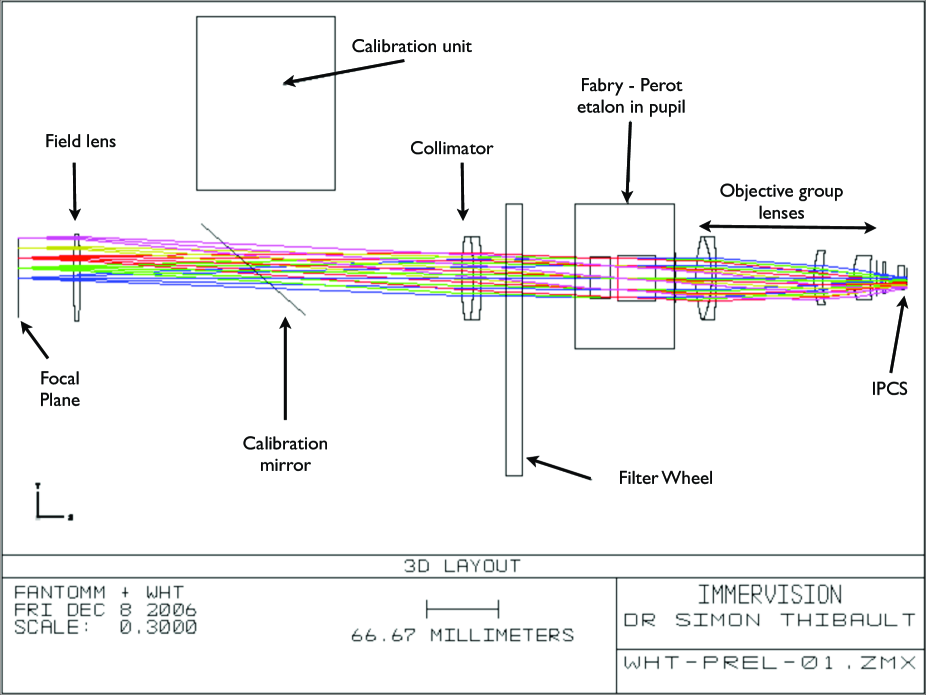
Figure 1: 2D optical layout of GH$\alpha$FaS. The optical design was done in collaboration with Immervision inc. Light beam from telescope comes from the left. The detector (IPCS) can been found at the right hand-side. Different colours of the optical rays represent different positions on the focal plane.

The spot diagram (Fig. 2) shows the optical performances of the instrument. It clearly stresses the size of the optical spot on the detector in various positions (conjugated of various positions on the sky). It is given for only a wavelength (6560Å) as observations are typically done in H$\alpha$  mode. The spot size is sampled by 1 pixel in the center and in alsmost the detector whereas 2 pixel are needed to have 50% of the encircled energy on the edges of the detector. The instrument is able to well sampled the seeing (typically 0.6”/px to 0.8”/px) with 2 pixels.

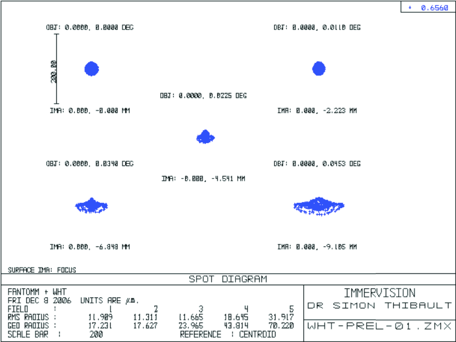
Figure 2: Spot Diagram of GH$\alpha$FaS in the detector plane for 5 different positions of the optical rays at a wavelength of 6560Å.

Table 3: GH$\alpha$FaS  Fabry-Perot etalons characteristics at H$\alpha$.

Etalon	pa	FSRb	$\Im^{c}$	$\Im^{d}_{e}$	Re
name		km s-1
Mégantic 1	765	391.9	22	17	16065
OM2	798	375.7	25	12	19950
OM3	2604	115.1	15	9	39060
OM4	609	492.3	30	24	18270
OM5	1938	154.7	56	32	108528
CFHT	1162	258.0	17	12	19754

The mechanical design was performed at the Université de Montréal. All parts are made of aluminium. The lens’ cylinders were painted inside to avoid any parasite reflection and included different masks. Lenses have been tested with a Zygo interferometer to check their quality. The optical and mechanical integration were done at Montreal, whereas the IPCS / Focal reducer integration was done at Marseille. Figure (Fig. 3) presents a top view and a cut along the optical axis parallel to the optical breadboard of the instrument on the optical table of the GHRIL.

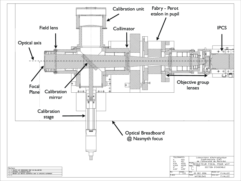
Figure 3: Top view and cut along the optical axis parallel to the optical breadboard at the Nasmyth focus. The optical and mechanical design of GH$\alpha$FaS has been especially customized for the GHRIL Nasmyth focus of the WHT. The filter wheel can fit four 75 mm-size filters and like all the elements of the system can be controlled remotely via ethernet cables.

Finally, the calibration arm, with its mirror controlled arm, has a neon lamp for calibration purpose. The Ne [6598] emission is used to calibrate the phase shifts of the Fabry Perot etalon. This lamp will be replaced, at a later stage, by a Photon etc Tunable Source (see www.photonetc.com) which is able to provide any calibration wavelength.

GH$\alpha$FaS is fully automated and controlled via ethernet modules. Table 4 presents a summary of all automated items in their operation modes. The filter wheel, the shutter, and the calibration arms have their own ethernet modules designed by Jean-Luc Gach and Philippe Ballard from LAM. The IPCS has its own dedicated link and network to avoid a mixing of the information between ethernet modules and data. The etalon is controlled via a RS-232 link with its CS100 controller.

Table 4: Summary of the GH$\alpha$FaS automated parts

Part name	Controlled by :	Operation
Calibration arm	ethernet module	calibration
Calibration lamp	ethernet module	calibration
Calibration mirror	ethernet module	calibration
Calibration stage	ethernet module	calibration
Fabry Perot Etalon	CS 100 via RS 232	observation & calibration
Filter wheel	ethernet module	observation & calibration

3.2 Detector: state of the art IPCS

3.2.1 IPCS

The IPCS is composed of a photocathode placed in front of a commercial CCD which amplifies the photons (from a factor 10⁵ to 10⁷, (see Gach et al. (2002) and Hernandez et al. (2003), and references therein for a complete description and history of such devices). It provides a system where the detection of a photon is around 10⁶ times above the readout noise of the commercial CCD. Therefore, the IPCS has essentially no readout noise.

The photocathode in the WHT camera is a GaAS type HAMAMATSU V7090-61 with a quantum efficiency of $<\sim$26% (this value includes the loss due to the MCP stack). The spectral range is from 400nm to 850nm and it is very flat over these wavelengths. It uses two microchannel plates to provide an electron amplification (after the photoelectic effect that converts photons to electrons) of 10⁷ (see figure 4). Each channel is 6 $\mu m$ wide.

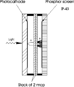
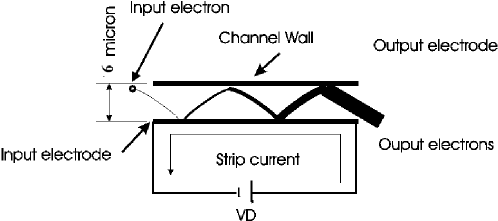
Figure 4: Left: Principle of electron amplification using micro channel plates (MCP) in an image intensifier. Right: Details of high voltage effect on a micro channel.

Finally, the electrons are projected onto a P-43 phosphor screen via a bundle of optical fibers and then is imaged on the focal plane of a DALSA fast readout commercial CCD (Panthera 1M60) using two objectives (from LINOS technology). Data are then transferred to an acquisition computer using the ”camera link” cable via an optical hub and to a dedicated ethernet link at 1Gbits/s (Balard et al. 2006).

3.2.2 Cooling System : the PELTIER Effect Simplified

A simple commercial PELTIER effect system is used to cool down the photocathode to its optimal temperature which is $-30^{o}$C. This PELTIER effect system is also coupled with a liquid cooling system to evacuate heat from the IPCS. The Dalsa CCD do not need to be cooled as photons (electrons) are amplified and well above the readout noise. The mean thermal noise of the cathode is 5 events/frame at $-10^{o}$C, which is equivalent to 0.7 photon/hour/pixel and drops to 3 events/frame at $-30^{o}$C. This dark current should drop to 0.4 events/frame if it was due only to the thermal emissivity of the photocathode. This background noise, which shows no dependence on temperature, can be explained by K⁴⁰ beta disintegration, which is present in the MCP glass (Siegmund et al., 1988). Recent investigations carried out in collaboration with Biospace lab company showed that using intensifier input windows free of potassium decreases the minimal background noise achievable by a factor of 10.

3.3 IPCS Advantages

The read-out noise affects CCDs at low light levels when very faint flux objects are observed. Classical CCDs reach nowadays high quantum efficiency (up to 95%), and very low read-out noise (down to 2-3 electrons and may be 1 in a near future, Gach et al. (2003)). With the IPCS, observations of faint flux objects are splitted into several short ones (in particular, this method also helps not to be severely polluted by cosmic rays). Thus, the maximal signal-to-noise ratio (SNR) per pixel achievable by an ”ideal” CCD is described by :

$$SNR=\frac{N}{\sqrt{N+n\sigma^{2}+T}},$$ (1)

where $N$ is the number of photons collected per pixel during the exposure time, $\sigma$ the readout noise of the CCD in electrons and $T$ the thermal noise in electrons/pixel. Although the $T$ term is close to zero in more recent CCD or IPCS devices and can be neglected, additional limitations constrain the usage of CCDs. $n$ is the number of exposures. The $SNR$ decreases dramatically when $N$ is small and $n$ is large. This is the case in multiplex instruments (scanning instruments). For an IPCS, the S/N is described by the following formula:

$$SNR=\frac{N}{\sqrt{N+T}}\approx\sqrt{N}.$$ (2)

As IPCS, in fact, do not have readout noise, they are also less affected by cosmic rays since one event is seen as one photon only, a decisive advantage with respect to CCDs, where long exposures are required in the case of faint objects. Although the first generation of IPCS had a poorer quantum efficiency with respect to CCDs and were affected by image distortion, they were still competitive in multiplex instruments or in speckle interferometry because of the absence of read-out noise.

Multiplex instruments collect a large number of images. For example, the scanning Fabry–Perot FaNTOmM  uses up to 64 channels to reconstruct the interferometric map of an object emission line, in order to determine its velocity field, monochromatic image, and velocity dispersion maps (see Hernandez et et al., 2003). The global SNR of a multiplex observation ($SNR_{m}$) is the quadratic sum of the SNRs of each channel, since there is no noise correlation between channels. Neglecting thermal noise , the SNR_m is given by :

$$SNR_{m}=\sqrt{n\left(\frac{\frac{N}{n}}{\sqrt{\frac{N}{n}+\sigma^{2}}}\right)^{2}}=\frac{N}{\sqrt{N+n\sigma^{2}}},$$ (3)

where $N$ is the number of photons expected during the whole exposure, $n$ is the number of channels and $\sigma$ is the readout noise of the CCD.

During multiplex observations, the emission usually appears only in a few channels, which could be different for each pixel according to the Doppler shift. Experiences with CIGALE and FaNTOmM  showed that, emission lines appear most of the time in only 25% of the channels. This lowers the above ”ideal” $SNR_{m}$. The ”worst” case is when the line is detected only in 2 channels. This does not affect the comparison between CCD and IPCS usage, but gives a more precise idea of the kind of objects that could be observed with such instruments. In this ”worst” case the $SNR_{m}$ is given by:

$$SNR_{m}=\sqrt{2\left(\frac{\frac{N}{n}}{\sqrt{\frac{N}{n}+\sigma^{2}}}\right)^{2}}=\frac{\frac{2N}{n}}{\sqrt{\frac{2N}{n}+2\sigma^{2}}}.$$ (4)

Because of the very small readout time (10 ms with the WHT camera and 25ms with the FaNTOmM  one) in the case of an IPCS, it is possible to observe each channel several times during the observation, then averaging the sky variations (since the first and last images may not be comparable in terms of seeing and transparency when observing with a groundbased telescope). Typically, each channel is observed 5 to 15 seconds, and when the last channel has been integrated, the first is observed again. Each set of $n$ channels is called a cycle, the duration of which is typically 5 to 15 minutes (depending on the exposure time per channel and the number of channels). The cycle exposure time must be under the OH timescale variations (typically 15 minutes, see Ramsay et al. 1992). Individual cycles are then summed to obtain the S/N ratio required without any loss of events. Many short cycles are then preferred to a single cycle with sky variation. The overlay time of the data acquisition system is under 10ms, so an exposure time of, at least, 1 s per channel, e.g. 48 s per cycle, is the shortest optimal exposure time. The experience of the LAE and LAM teams lead channel exposure time to 5 s, so a cycle time of around 5 minutes. The total observation consists of several cycles. SNR_m can be rewritten as :

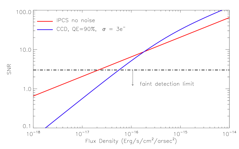
Figure 5: Signal to noise ratio comparison: IPCS and CCD at the WHT. The red line shows the SNR for an IPCS, for a 3 hour exposure of 40 cycles with 48 channels, on a 4.2m telescope with a pixel size of 0.5” assuming a trough-put of the telescope of 80%. The blue line shows the SNR of a scientific grade CCD with a QE of 90% and a readout noise ($\sigma$) of 3$e^{-}$ in the same exposure conditions. The faint detection limit is placed at a SNR of 3.

$$SNR_{m}=\frac{\frac{2N}{n}}{\sqrt{\frac{2N}{n}+2m\sigma^{2}}},$$ (5)

where $N$ is the number of photons expected during the whole exposure, $n$ the number of channels, $m$ the number of cycles and $\sigma$ the readout noise of the CCD. Meanwhile, the IPCS $SNR_{m}$obtained is independent of the number of cycles and the atmosphere-free SNR is:

$$SNR_{m}=\sqrt{\frac{2N}{n}}.$$ (6)

These two equations are used to generate figure 5. The faint detection limit is for a SNR of 3. It can be seen on this figure, that an IPCS can reach higher SNR than a classical CCDs for very faint fluxes.

The measured QE of the whole system (including MCP losses) was measured to be 26% at H$\alpha$. The overall system presents the same characteristics as the IPCS of FaNTOmM  (Gach et al. (2002) and Hernandez et al. (2003)). The system is limited by the process itself. The Dalsa camera can be read with two speeds depending on the binning mode (1024x1024px or 512x512px) chosen. When two events occur within the same frame (16.6 ms or 10 ms ) at the same location, only one event is counted instead of two. The mean number M of missed photons can be evaluated assuming a Poissonian process for the photon emission by the following equation :

$$M=N\times(1-\frac{1-e^{-\lambda}}{\lambda}),$$ (7)

where $\lambda=N/$frame per second, is the mean number of photons expected during the resolved period of the detector and $N$ the total number of photons.

Figure 6 shows the percentage of non-linearity of an IPCS detector at different possible frame rates. This shows that the system loses its linearity when the flux increases. Therefore this detector is used exclusively for faint fluxes. Figure 6 shows also that this effect is less important for higher frame rates. The blue lines (dot or continuous) represent the FaNTOmM  GaAs system, and the red one is the improved GH$\alpha$FaS  camera.

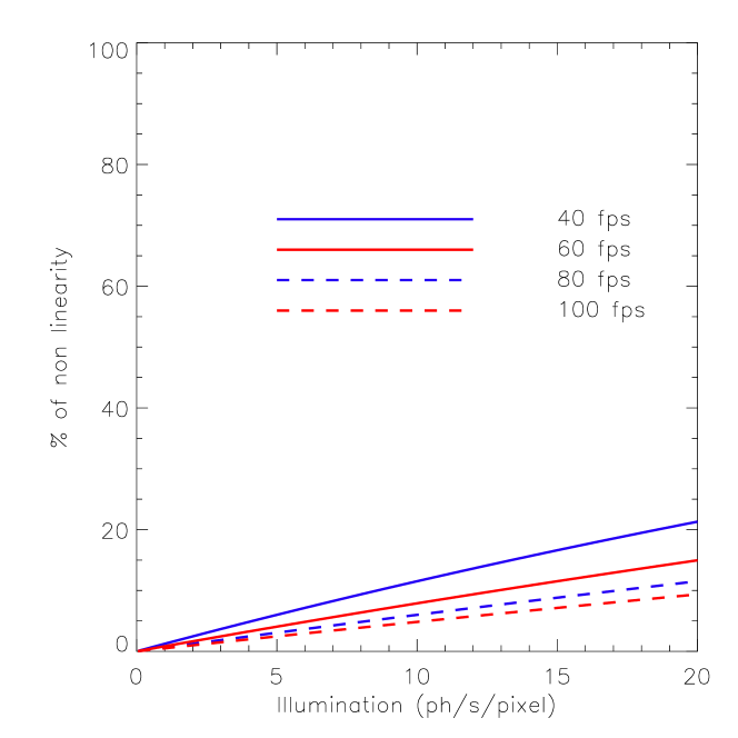
Figure 6: Computed non-linearity of an IPCS detector at different frame rates.

4 Data Reduction

4.1 Data Preparation

As GH$\alpha$FaS is mounted on the optical table of the Nasmyth focus, our observations are affected by the field rotation. The optical derotator provided by the Isaac Newton Group (ING) of Telescopes has the disadvantage of covering a field of only $2.5\arcmin\times 2.5\arcmin$, which is too small for the scientific programs envisaged for GH$\alpha$FaS. Our observation strategy allows us to store the image of the individual channel separately, which is ideal for derotating the observed cube a posteriori. Following the information provided on the ING web pages, the field rotation is $\approx 0.29$″, i.e., negligible, during the exposure of each individual cycle ($\sim 4$ minutes).

Most of the data reduction steps are carried out using an IDL based data reduction package developed by Daigle et al. (2006). However, since we do not use the optical derotator, the data are affected by the rotation. In order to correct for this effect, we combine Daigle’s reduction package with a number of available packages, KARMA, SWARP and IMWCS. The complete steps of the GH$\alpha$FaS  data reduction are:

1. An initial and rough estimate of the data quality by reducing the observed data cube. This step allows also a good phase calibration which we use to reduce the individual cycles.

2. Individual reduction of each observed cycle.

3. Creating a cube image for each reduced cycle. Investigating each of these images, we have found that for almost all the observed galaxies, the effect of the sky rotation is marginal within the 4 minutes exposure to scan one cycle. This is also confirmed by the ING web pages.

4. The collapsed cube image of each individual cycle is then used to find the three brightest point sources. The IMWCS and KARMA tools are then used to include the appropriate keywords in the header of each image.

5. We found that a simple rotational transformation does not provide the adequate accuracy, hence we use the SWARP package to match all cycles regardless of the complexity of the transformation required.

6. We apply the same transformation to each individual channel within each cycle, and re-build a corrected version of the data cube.

7. Finally, we reduce the corrected data cube following all the standard reduction procedures presented in Daigle et al. (2006).

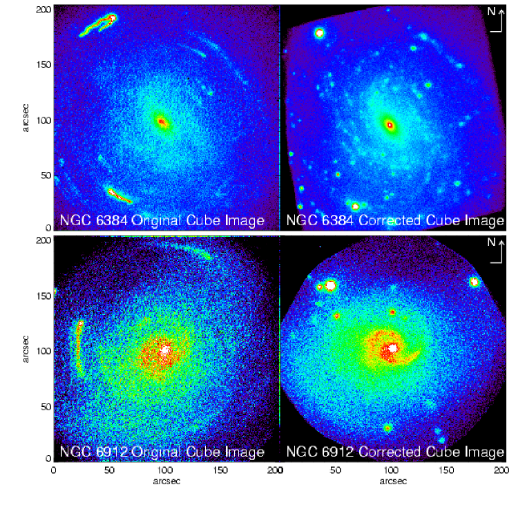
Figure 7: Examples of derotation

Note that this process is made possible only because our detector has a high time resolution and has no readout noise. This reduction process does not add any excess noise to the observational data and keeps the very high overall sensitivity of the instrument.

4.2 Data Reduction and Derivation of the H$\alpha$  Kinematics

GH$\alpha$FaS data reduction involves the standard Fabry-Perot data reduction steps: cube construction, phase calibration, sky subtraction, and kinematics derivation, which is done using the software package of Daigle et al. (2006) and the GIPSY package (Vogelaar & Terlouw, 2001).

By construction, GH$\alpha$FaS  covers a reasonably large field in order to observe nearby extended objects and provide simultaneous sky coverage to allow for reliable sky subtraction. However, some galaxies extend beyond the full GH$\alpha$FaS field. In order to sample the sky variations properly during the long observation of the object, the telescope is pointed to a blank field away from the galaxy, once every three cycles. The sky cubes are thereafter treated in the same way as the galaxy cube. The reduced sky cube is then re-scaled to the galaxy count level and subtracted from the galaxy cube. In order to examine the accuracy of the sky subtraction procedure, the sky cube is used in four different ways before subtraction from the galaxy. All the sky spectra are then rearranged to build one spectrum representative of the entire sky cube, but also fitted with 1st, 3rd and 4th order polynomials to each channel image of the sky cube. Subtracting each sky representation separately, we end up with four different reduced galaxy cubes.

The free spectra range FSR determines the depth of the data cube and is a function of the observed wavelength ($\lambda$) and the interference order ($p$) at this wavelength. $FSR=\lambda/p$. The number of channels is linked to the finesse of the Airy function of the etalon (in fact, the number of channel respects the Nyquist criteria : n = 2.2 $\times$ the effective Finesse) and has no relation with the FSR. To study normal galaxies, a FSR of 0.8nm (360 kms at H$\alpha$) is used. If the velocity range of a galaxy (with its inclination factor) is larger than the FSR (which is not frequent), one will find in order -1 or +1 the rest of the velocity field (filters, used in front of the etalon, typically block all etalon order except $p+1,p,p-1$). So a jump in the velocity field is generally found and easily corrected. This could happen with active galactic nuclei of galaxy. In that particular case, an other etalon is used to increase the FSR. Table 2 presents the FSR for different etalons.

Each reduced galaxy cube is treated independently to derive the H$\alpha$   kinematics by means of deriving the moment maps with consistency checks by applying single Gaussian profiles to the spectra (e.g., Fathi et al. 2007a). Analyzing the kinematical maps, it was found that the sky subtraction does not significantly change the derived kinematics. In order to gain more field coverage, a two-dimensional Voronoi tessellation method (Cappellari & Copin 2003, Daigle et al 2006) was applied on the faint regions of the observed field. Finally, the maps are cleaned by removing all values which are derived from spectra with amplitude-over-noise ($A/N$) less than 10 (the noise being the standard deviation of the parts of the spectra outside the H$\alpha$   emission line). Although this seems a strict criterion, it was chosen to continue the analysis of the velocity field based on spectra which are reliable not only for deriving reliable velocities, but also velocity dispersion. GH$\alpha$FaS instrumental dispersion has been measured using the Neon lamp and was found to be $\sigma_{\mathrm{inst}}=FWHM/2.35=2.5$  km s^-1 . It was then subtracted quadratically from the H$\alpha$   velocity dispersion, and the derived velocities were corrected for the Heliocentric velocity drift.

To give an idea of the efficiency of the pipeline reduction, two panels of results are given, representing the scientific drivers of the instrument. The final kinematical maps are presented in the appendix section in Fig. 8 for four objects while H$\alpha$  monochromatic images are represented in Fig 9. Finally,monochromatic image in the [NII] line and the first order of the PNe M1-75 is presented in Fig 10. This is not the goal of this paper to comment, analyse or derive kinematical parameters. The final, complete and detailed data reduction and analysis will be available in forthcoming papers.

Finally, the status of the data reduction of the first run (17 objects !) over 6 nights are presented in Table 5.

Table 5: Observed Objects with GH$\alpha$FaS during 6 nights

Name	R.A.	Dec.	Vsys	Night	$\langle$Seeing$\rangle$	Status
NGC 4376	12 25 18.0	+05 44 28	1136	6	0.7	Reduced
NGC 4594	12 39 59.4	-11 37 23	1024	4	2.0	Reduced
NGC 5236	13 37 00.9	-29 51 57	513	5	0.7	Reduced
NGC 5427	14 03 26.0	-06 01 51	2618	2	1.5	Reduced
NGC 5850	15 07 07.7	+01 32 39	2556	3	2.0	Reduced
NGC 5954	15 34 35.1	+15 11 54	1959	2	1.5	Reduced
NGC 6118	16 21 48.6	-02 17 00	1573	6	0.6	Reduced
NGC 6384	17 32 24.3	+07 03 37	1665	1	1.8	Reduced
NGC 6643	18 19 46.4	+74 34 06	1484	2	1.5	In progress
NGC 6643	18 19 46.4	+74 34 06	1484	2	Imaging	In progress
NGC 6912	20 26 52.1	-18 37 02	6968	3	2.5	Reduced
NGC 6912	20 26 52.1	-18 37 02	6968	6	0.8	Reduced
NGC 6962	20 47 19.1	+00 19 15	4211	4	1.8	Reduced
KPG 552	21 07 44.0	+03 52 30	7767	5	0.6	Reduced
KPG 591	23 47 01.6	+29 28 17	4845	4	1.5	Reduced
PN M1-75	20 04 44.1	+31 27 24	${\ddagger}$3890	5	0.8	Reduced
Arp 278	22 19 28.6	+29 23 32	4718	6	0.8	Reduced

5 Conclusions

GH$\alpha$FaS , a new Fabry-Perot system with high spatial and spectral resolution has been presented. GH$\alpha$FaS offers the largest FOV of such instrument on a 4m class telescope. It is also the most versatile instrument capable to study ISM to high redshift galaxies.

GH$\alpha$FaS provides a FOV of 202”$\times$202” with two spatial resolutions: 0.4”/px or 0.2”/px (hard-binned mode). Different spectral resolutions can be achieved simply by changing etalon in the pupil space. With the actual bank of etalon available, spectral resolution varies from 8000 to 110000. The use of tunable filters (in development both at LAE and LAM) would also improve the versatily of this instrument. The high performance no readout-noise detector, in the GH$\alpha$FaS version, remains the best detector to be used with faint fluxes science cases. It allows, at the same time, real-time data acquisition (astronomical object is seen in live during observation), on sky reduction and real-time OH sky lines removing. Finally, a robust reduction pipeline, for complete data reduction is available and can be obtained at www.astro.umontreal.ca/fantomm/reduction.

Developing of GH$\alpha$FaS was formulated in the summer of 2006 by the IAC and conception, design and realization began in the beginning of 2006 December at LAE. The first lights were obtained only 6 months later in 2007 summer. This fast schedule was possible because of th=e expertise developed at LAM, Observatoire de Marseille, and LAE at University of Montreal, through the building of FaNTOmM and CIGALE. While GH$\alpha$FaS was constructed as a private instrument, it is expected to become a visitor instrument at WHT in less than two years.

GH$\alpha$FaS should be considered as an high-performance instrument but also as a lab test of much more complicated instruments such as the 3D-NTT (www.astro.umontreal.ca/3dntt), the Brazilian Tunable Filter : BTFi (www.astro.iag.usp.br/$\sim$btfi) and the smart tunable Filter for the E-ELT (Moretto et al. 2006). Those instruments will use GH$\alpha$FaS technology but with many improved features, such as EMCCD (Daigle et al. 2007), customs large tunable filters and new Tunable filter made with Volume Phase gratings (Blais-Ouellette et al. 2006).

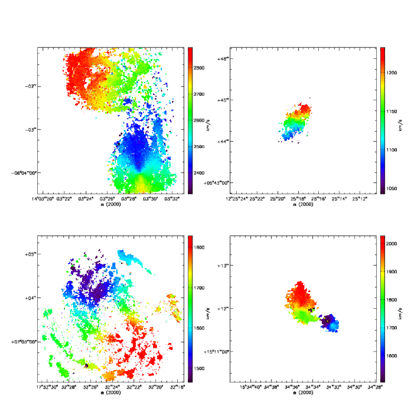
Figure 8: Kinematical maps of 4 objects.Top left: NGC 5427 with NGC 5426.Top rigth: NGC 4376.Bottom Left: NGC 6384. Botton right: NGC 5954 with NGC 5953

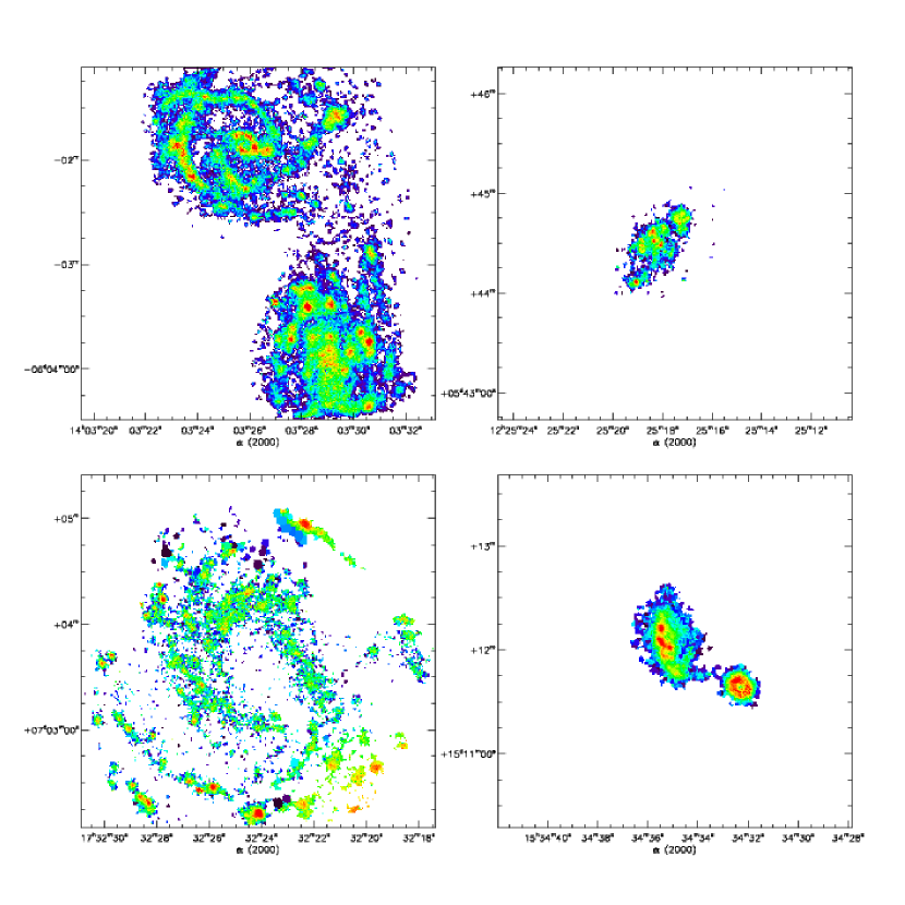
Figure 9: H$\alpha$  images of 4 objects.Top left: NGC 5427 with NGC 5426.Top rigth: NGC 4376.Bottom Left: NGC 6384. Botton right: NGC 5954 with NGC 5953

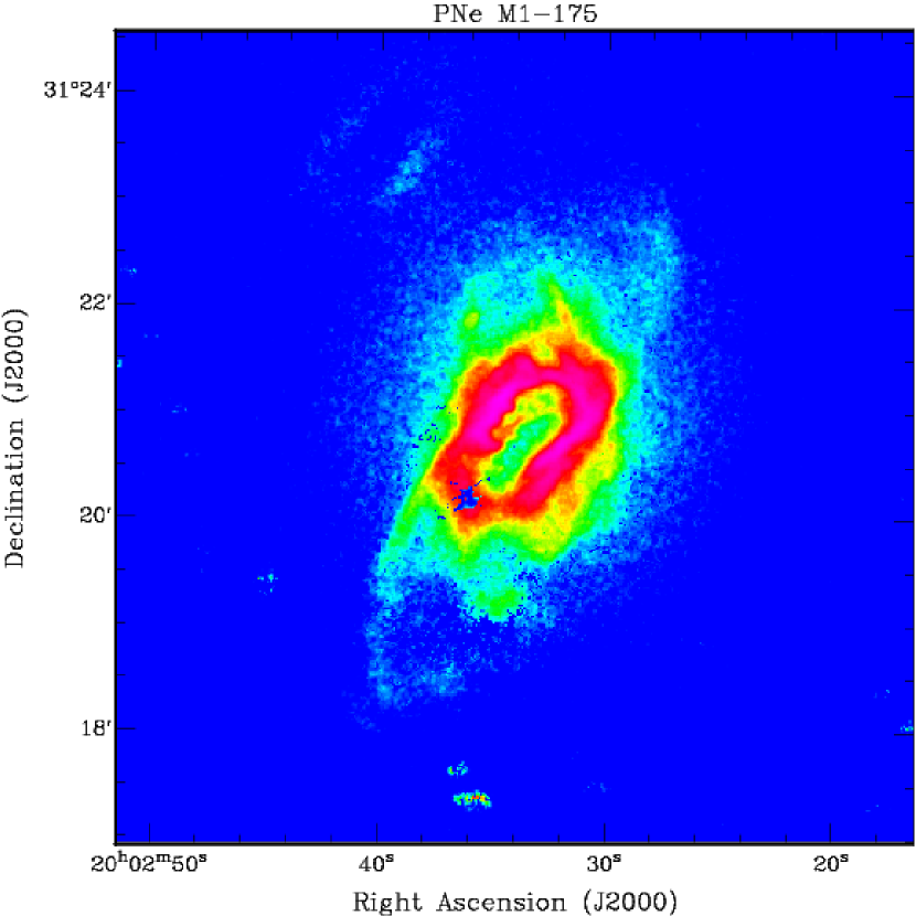
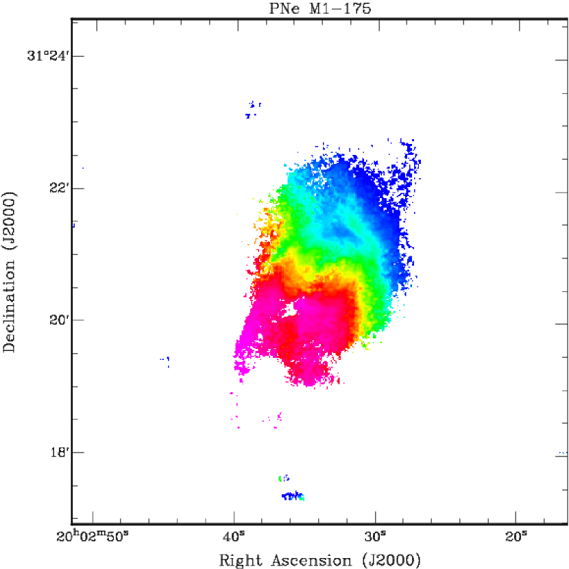
Figure 10: Left: [NII]658.3 nm image of Planatary Nebula M1-75 with a pixel size of 0.2”. Right: associated expansion velocity field. Range of velocity is from 76  km s^-1 to 231  km s^-1

References

- Amram et al. (2007) Amram, P., Mendes de Oliveira, C., Plana, H., Balkowski, C., & Hernandez, O. 2007, A&A, 471, 753
- Amram et al. (2004) Amram, P., et al. 2004, ApJ, 612, L5
- Arribas et al. (1998) Arribas, S., et al. 1998, Fiber Optics in Astronomy III, 152, 149
- Athanassoula (2005) Athanassoula, E. 2005, Celestial Mechanics and Dynamical Astronomy, 91, 9
- Atherton et al. (1982) Atherton, P. D., Taylor, K., Pike, C. D., Harmer, C. F. W., Parker, N. M., & Hook, R. N. 1982, MNRAS, 201, 661
- Bacon et al. (1995) Bacon, R., et al. 1995, A&AS, 113, 347
- Bacon et al. (2001) Bacon, R., et al. 2001, MNRAS, 326, 23
- Balard et al. (2006) Balard, P., et al. 2006, Scientific Detectors for Astronomy 2005, 117
- Balick & Frank (2002) Balick, B., & Frank, A. 2002, ARA&A, 40, 439
- Blais-Ouellette et al. (2004) Blais-Ouellette, S., Guzman, D., Elgamil, A., & Rallison, R. 2004, Proc. SPIE, 5494, 278
- Bland et al. (1990) Bland, J., Tully, R. B., & Cecil, G. N. 1990, Proc. SPIE, 1235, 590
- Boulesteix et al. (1984) Boulesteix, J., Georgelin, Y., Marcelin, M., & Monnet, G. 1984, Proc. SPIE, 445, 37
- Cappellari & Copin (2003) Cappellari, M., & Copin, Y. 2003, MNRAS, 342, 345
- Chemin et al. (2006) Chemin, L., Balkowski, C., Cayatte, V., Carignan, C., Amram, P., Garrido, O., Hernandez, O., Marcelin, M., Adami, C., Boselli, A., & Boulesteix, J. 2006, MNRAS, 366, 812
- Chu & Kennicutt (1994) Chu, Y.-H., & Kennicutt, R. C., Jr. 1994a, ApJ, 425, 720
- Chu & Kennicutt (1994) Chu, Y.-H., & Kennicutt, R. C., Jr. 1994b, Ap&SS, 216, 253
- Courtes (1982) Courtes, G. 1982, IAU Colloq. 67: Instrumentation for Astronomy with Large Optical Telescopes, 92, 123
- Curtis (1918) Curtis, H. D. 1918, Publ. Lick. Obs.; Vol. 13; Page 45-54, 13, 45
- Daigle et al. (2006) Daigle, O., Carignan, C., Amram, P., Hernandez, O., Chemin, L., Balkowski, C., & Kennicutt, R. 2006, MNRAS, 367, 469
- Daigle et al. (2006) Daigle, O., Carignan, C., Hernandez, O., Chemin, L., & Amram, P. 2006, MNRAS, 368, 1016
- toto3 (2006) Dekel & Birnboin 2006, MNRAS, 368, 2
- de Zeeuw et al. (2002) de Zeeuw, P. T., et al. 2002, MNRAS, 329, 513
- Dopita et al. (2007) Dopita, M., Hart, J., McGregor, P., Oates, P., Bloxham, G., & Jones, D. 2007, Ap&SS, 310, 255
- Eisenhauer et al. (2003) Eisenhauer, F., et al. 2003, Proc. SPIE, 4841, 1548
- Fathi et al. (2007) Fathi, K., Beckman, J. E., Zurita, A., Relaño, M., Knapen, J. H., Daigle, O., Hernandez, O., & Carignan, C. 2007, A&A, 466, 905
- Fathi et al. (2007) Fathi, K., Toonen, S., Falcón-Barroso, J., Beckman, J. E., Hernandez, O., Daigle, O., Carignan, C., & de Zeeuw, T. 2007, ApJ, 667, L137
- Fathi et al. (2005) Fathi, K., van de Ven, G., Peletier, R. F., Emsellem, E., Falcón-Barroso, J., Cappellari, M., & de Zeeuw, T. 2005, MNRAS, 364, 773
- Fathi & Peletier (2003) Fathi, K., & Peletier, R. F. 2003, A&A, 407, 61
- Flores et al. (2006) Flores, H., Hammer, F., Puech, M., Amram, P., & Balkowski, C. 2006, A&A, 455, 107
- Förster Schreiber et al. (2006) Förster Schreiber, N. M., et al. 2006, ApJ, 645, 1062
- Gach et al. (2002) Gach, J.-L., Hernandez, O., Boulesteix, J., Amram, P., Boissin, O., Carignan, C., Garrido, O., Marcelin, M., Östlin, G., Plana, H., & Rampazzo, R. 2002, PASP, 114, 1043
- Gach et al. (2003) Gach, J.-L., Darson, D., Guillaume, C., Goillandeau, M., Cavadore, C., Balard, P., Boissin, O., & Boulesteix, J. 2003, PASP, 115, 1068
- García-Segura et al. (1999) García-Segura, G., Langer, N., Różyczka, M., & Franco, J. 1999, ApJ, 517, 767
- Genzel et al. (2006) Genzel, R., et al. 2006, Nature, 442, 786
- Gonçalves et al. (2006) Gonçalves, D. R., Ercolano, B., Carnero, A., Mampaso, A., & Corradi, R. L. M. 2006, MNRAS, 365, 1039
- Haehnelt & Kauffmann (2000) Haehnelt, M. G., & Kauffmann, G. 2000, MNRAS, 318, L35
- Henault et al. (2004) Henault, F., et al. 2004, Proc. SPIE, 5492, 909
- Hernandez et al. (2005) Hernandez, O., Carignan, C., Amram, P., Chemin, L., & Daigle, O. 2005, MNRAS, 360, 1201
- Hernandez et al. (2005) Hernandez, O., Wozniak, H., Carignan, C., Amram, P., Chemin, L., & Daigle, O. 2005, ApJ, 632, 253
- Hernandez et al. (2003) Hernandez, O., Gach, J.-L., Carignan, C., & Boulesteix, J. 2003, SPIE, 4841, 1472
- Hill et al. (2006) Hill, G. J., et al. 2006, Proc. SPIE, 6269,
- Kaufer et al. (2003) Kaufer, A., Pasquini, L., Castillo, R., Schmutzer, R., & Smoker, J. 2003, The Messenger, 113, 15
- toto5 (2006) Kauffmann et al. 2003, MNRAS, 341, 54
- toto6 (2006) Klypin et al. 1999, ApJ, 522, 82
- Maciejewski (2006) Maciejewski, W. 2006, MNRAS, 371, 451
- Maciejewski & Athanassoula (2007) Maciejewski, W., & Athanassoula, E. 2007, MNRAS, 380, 999
- Marquart et al. (2007) Marquart, T., Fathi, K., Östlin, G., Bergvall, N., Cumming, R. J., & Amram, P. 2007, A&A, 474, L9
- Moe & De Marco (2006) Moe, M., & De Marco, O. 2006, ApJ, 650, 916
- Moretto et al. (2006) Moretto, G., et al. 2006, Proc. SPIE, 6269
- toto7 (2006) Newman & Davis 2002, ApJ, 564, 567
- Peletier et al. (2007) Peletier, R. F., et al. 2007, MNRAS, 379, 445
- Primack (2006) Primack, J. R. 2006, ArXiv Astrophysics e-prints, arXiv:astro-ph/0609541
- Ramsay et al. (1992) Ramsay, S. K., Mountain, C. M., & Geballe, T. R. 1992, MNRAS, 259, 751
- Relaño et al. (2007) Relaño, M., Beckman, J. E., Daigle, O., & Carignan, C. 2007, A&A, 467, 1117
- Relaño & Beckman (2005) Relaño, M., & Beckman, J. E. 2005, A&A, 430, 911
- Relaño et al. (2005) Relaño, M., Beckman, J. E., Zurita, A., Rozas, M., & Giammanco, C. 2005, A&A, 431, 235
- Rosado et al. (2007) Rosado, M., Arias, L., & Ambrocio-Cruz, P. 2007, AJ, 133, 89
- Rozas et al. (2006) Rozas, M., Richer, M. G., López, J. A., Relaño, M., & Beckman, J. E. 2006, A&A, 455, 549
- Siegmund (1988) Siegmund, O. H. W. 1988, Proc. SPIE, 982, 108
- Shlosman et al. (1989) Shlosman, I., Frank, J., & Begelman, M. C. 1989, Nature, 338, 45
- Sluis & Williams (2006) Sluis, A. P. N., & Williams, T. B. 2006, AJ, 131, 2089
- Thatte et al. (2006) Thatte, N., Tecza, M., Clarke, F., Goodsall, T., Lynn, J., Freeman, D., & Davies, R. L. 2006, Proc. SPIE, 6269
- Terlevich & Melnick (1981) Terlevich, R., & Melnick, J. 1981, MNRAS, 195, 839
- Tremaine et al. (2002) Tremaine, S., et al. 2002, ApJ, 574, 740
- Vogelaar & Terlouw (2001) Vogelaar M. G. R., Terlouw J. P., 2001, ASPC, 238, 358
- Zurita et al. (2001) Zurita, A., Rozas, M., & Beckman, J. E. 2001, Ap&SS, 276, 491
- Zurita et al. (2004) Zurita, A., Relaño, M., Beckman, J. E., & Knapen, J. H. 2004, A&A, 413, 73