Quasar candidates selection in the Virtual Observatory era

Abstract

We present a method for the photometric selection of candidate quasars in multiband surveys. The method makes use of a priori knowledge derived from a subsample of spectroscopic confirmed QSOs to map the parameter space. The disentanglement of QSOs candidates and stars is performed in the colour space through the combined use of two algorithms, the Probabilistic Principal Surfaces and the Negative Entropy clustering, which are for the first time used in an astronomical context. Both methods have been implemented in the VONeural package on the Astrogrid VO platform. Even though they belong to the class of the unsupervised clustering tools, the performances of the method are optimized by using the available sample of confirmed quasars and it is therefore possible to learn from any improvement in the available ”base of knowledge”. The method has been applied and tested on both optical and optical plus near infrared data extracted from the visible SDSS and infrared UKIDSS-LAS public databases. In all cases, the experiments lead to high values of both efficiency and completeness, comparable if not better than the methods already known in the literature. A catalogue of optical candidate QSOs extracted from the SDSS DR7 Legacy photometric dataset has been produced and is publicly available at the URL http://voneural.na.infn.it/qso.html.

1 Introduction

Over the years, serendipitous discoveries and systematic searches have caused the number of confirmed quasars to grow dramatically, but we are still far from having discovered even a significant fraction of the $\sim$ 1.6 million QSOs which are expected to populate the universe out to $z\simeq 3$ (e.g. [Richards et al. 2004]). Thanks to their high intrinsic brightness, such lack of coverage is not due to the limited depth of the observations aimed at discovering QSOs, but mainly to the difficulties encountered, first in disentangling normal stars from QSO candidates, and then in confirming their nature through additional data (such as spectroscopy, radio or X-ray fluxes) which are usually either difficult or very time-consuming to provide for statistically significant samples of objects. This is very unfortunate since, as it has been stressed by many authors [Richards et al. 2002, Richards et al. 2004], sizeable samples of quasars covering a broad range of redshifts and selected with uniform and well controlled criteria, are greatly needed to address many relevant issues such as the evolution of the quasar luminosity function or the spatial clustering of quasars as a function of the redshift.

The most notable recent efforts at building extensive samples have been the quasars searches in the Sloan Digital Sky Survey (hereafter SDSS, [York et al. 2000]) and the main competing project, the 2dF QSO redshift survey [Croom et al. 2001] which will soon be joined by ongoing or planned multiband photometric survey projects such as, for instance, the Palomar Quest [Djorgovski et al. 2004], or the VST [Capaccioli et al. 2003] and VISTA [McPherson et al. 2006] surveys. From the photometric standpoint, all quasar candidates selection algorithms are based on a few simple facts:

1. the spectral energy distribution of stars is roughly blackbody in shape, while quasars have SEDs that are characterized by featureless blue continua and strong emission lines. In particular, at low redshifts ($z\leq 2.2$), the lack of a Balmer jump in quasars separates them from hot stars; at higher redshifts the presence of a strong $Ly_{\alpha}$ emission line and of absorption by the $Ly_{\alpha}$ forest results in the broadband colours of quasars to become increasingly redder with redshift. These, in general, is the reason why quasars can be distinguished by stars when looking at their position in a colour space generated by observations in a broadband photometric system: stars and QSOs may have the same colour in some wavelength region, but the colours in the other regions will be different;

2. as stressed by [Richards et al. 2001], the overall shape of the continuum of quasars is well approximated by a power law. The combined effect of the different shapes of the continuum emission and the presence of spectral features not observed in stars is that QSOs show colours which vary significantly as a function of redshifts, but locally (in redshift) the distribution of colours is narrow and not-degenerate;

3. at high redshifts, the density of absorption lines in the spectral energy distribution of QSOs increases, so that, when the region of the quasar rest frame spectrum shortwards of 912 $\AA$ enters the observed band, absorption due to the intervening optically thick clouds further reddens the spectrum, causing the quasar to move away from the region of the colours space occupied by Galactic stars.

In the particular case of infrared wavelengths, the availability of large-field detectors on large field of view telescopes has provided the opportunity to undertake surveys capable of establishing the importance of the main mechanism of reddening, i.e. the extinction by dust, on the observed population of quasars. Since the spectral energy distributions of quasars vary significantly as a function of the wavelength, flux measurements at widely separated wavelengths are used to characterize fully the spectral properties of the quasar population. More precisely, two methods exploiting the differences between the power-law nature of quasar spectra and the convex spectra of stars have been proposed to select candidate quasars, based on the fact that quasars are significantly brighter than stars at both short wavelengths - the UVX method [Sandage & Wyndham 1965, Hewitt et al. 1993] - and long wavelengths - the KX method [Warren et al. 2000]. In order to build large samples of quasars a major goal is to improve the reliability and efficiency of the algorithms used to extract from multiband survey data the list of quasar candidates. Most current algorithms are typically more than 60% efficient for UV-excess (UVX) quasars at relatively bright magnitudes, but the selection efficiency drops at fainter magnitudes where the photometric errors are largest and most of the observable objects resides. As shown by [Richards et al. 2004], however, it is possible to build algorithms achieving levels of accuracy and completeness (for a definition of these terms see Section (3)) which can mitigate the need for confirming spectra. One additional fact that needs to be noticed is that the efficiency of all quasar candidate selection algorithms depends on some degree on the fine tuning of the algorithms on what we could call the a priori knowledge (hereafter ”Base of Knowledge” or BoK) of what quasars are and on what their main characteristics are. This BoK may be either built out of synthetic spectra or from available quasar samples. The latter approach, being based on fewer a priori assumptions, seems preferable but, on the other end, it keeps all biases introduced by the selection criteria (to be more explicit: if a specific subclass of objects is not present in the BoK, the algorithm will not be able to recognize them). In a near future, however, the large amount of data which will be made available to the community through the Virtual Observatory [Walton 2002], will provide an ever growing (both in size and accuracy) BoK which will allow to overcome at least some of the existing limitations. In this paper we present a method based on unsupervised clustering capable to map the photometric parameter space using the information contained in the BoK and to disentangle stars from candidate quasars. Finding candidate QSOs is only the first step in the process of the characterization of the distribution of such sources in the Universe, the second being the production of a three dimensional map of their position through the estimate of the redshifts for each of them. A method for the calculation of accurate photometric redshifts based on a machine learning approach similar in its philosophy to the one described in [D’Abrusco et al. 2007] and intended to complement the present QSOs candidate selection algorithm is in preparation, and will be discussed in a forthcoming paper by the same authors. Even though it is applied to the SDSS and/or UKIDSS public data, the method is of general validity and can be easily adapted to any other data set given that a proper BoK is available. It needs to be explicitly stressed that the effectiveness and accuracy of the method presented in this paper strongly depend on the completeness and accuracy of the assumed ”a priori” knowledge contained in the BoK, and, in this sense, this method does not overcome the biases contained in the BoK. However, with the advent of VO technology the quality and accuracy of the BoK’s is bound to increase dramatically, since the growing availability of federated data sets observed at different wavelengths will remove most of the systematic selection effects encountered in the current data and will improve the completeness of the selection of members of the BoK. In this respect, one of the main advantages of this particular method is that it can easily adapts to any improvement of the BoK. In section (2) we present the main characteristics of the data used for the experiments and in Section (3) we shortly summarize the main methods used so far for the selection of candidate QSOs from the SDSS catalogues. In Section (4) we introduce the clustering algorithm and the agglomerative method and in Section (5) we discuss the results of the experiments performed. The catalogue of optical QSO candidates extracted from ther SDSS photometric dataset and the base of knowledge used for the candidates selection are described in Section (7), while the conclusions are drawn in Section (8). Besides the experiment described in section (5), in order to guide the reader through the subtleties of the method presented here, in section (3), together with the theoretical aspects of the algorithms employed, an experiment performed on a simplified version of one of the data samples is described. A restricted BoK and a different set of parameters for the algorithms will be used as well for the sake of clarity. In two forthcoming papers [D’Abrusco et al., in prep., Cavuoti et al., in prep.] we shall discuss the application of the method to the selection of heavily obscured quasars and to the physical classification of AGNs, respectively.

2 The data

2.1 SDSS data

The Sloan Digital Sky Survey is a digital survey aimed at covering $\sim 10,000$ sq. deg. mainly in the Northern emisphere [Stoughton et al. 2002] in five specifically designed bands $(u,g,r,i,z)$ [Fukugita et al. 1996] and is complemented by an extensive redshift survey for about $10^{6}$ objects (mainly galaxies and QSOs). The SDSS data are made available to the community through a public archive which at the moment is distributing its Seventh Data Release Legacy Survey (hereafter DR7) [Abazajian et al. 2008]. So far, SDSS provides the best data set to date for those interested in mining for photometrically selected subsamples of objects. As such, it has been extensively studied in almost all its aspects and an impressive amount of literature has been produced providing an accurate knowledge of completeness, selection effects etc. [Adelman et al. 2007]. As to quasar selection from the SDSS data, it is worth to recall a few facts. The SDSS photometric system does not allow the detection of quasars with $z>6$ and; with the additional constraint of having the objects detected in at least two bands, this limit reduces to $z\sim 5.8$ [Fan et al. 2001b, Richards et al. 2002]. At the low- end, the design of the $u$ filter and the location of the gap between the $u$ and $g$ filters were chosen to emphasize the difference between objects with power-law spectral energy distributions (SEDs), such as quasars at $z<2.2$, and objects that are strongly affected by the Balmer decrement, in particular A stars, which are recognized as the prime contaminants in multicolor optical searches for low-redshift quasars.

2.2 UKIDSS data

The United Kingdom Infrared Deep Sky Survey (hereafter UKIDSS) [Lawrence et al. 2007], is a near-infrared sky survey that will cover $7500$ square degrees of the Northern sky, extending over both high and low Galactic latitudes, in $(Y,J,H,K)$ bands down to $K\simeq 18.3$, thus reaching three magnitudes deeper than 2MASS [Jarrett et al. 2000]. UKIDSS has been designed and operated to be the near-infrared counterpart of the SDSS survey; it is made up of five separate surveys and includes two deep extra-Galactic elements, one covering 35 square degrees down to $K=21$, and the other reaching $K=23$ over 0.77 square degrees of the sky. In this work we make use of the UKIDSS Large Area Survey (hereafter LAS) which aims at covering an area of 4,000 deg² overlapping with the SDSS. The LAS is expected to be completed in 2012, after an observing period of seven years. LAS is surveying the sky in four photometric bands $(Y,J,H,K)$ with typical limiting magnitudes $[20.5,20.0,18.8,18.4]$ and astrometric accuracy typically $<0^{{}^{\prime\prime}}.1$. The UKIDSS DR1 [Dye et al. 2006] release overlaps a subset of the SDSS northern and southern areas with photometric and astrometric performances similar to the SDSS.

2.3 The bases of knowledge

In this work, three different samples of objects were used as BoKs in order to evaluate the performances of our candidate selection algorithm with respect to the original SDSS quasars candidate selection technique (see paragraph (3.1)) and the algorithm proposed by Richards and his collaborators [Richards et al. 2004] (see paragraph (3.2)) respectively. The first and third datasets (S-A and S-S) employ only optical photometric and spectroscopic data from the SDSS survey, while the second dataset (S-UK), despite based on the same spectroscopic classification provided by Sloan database, uses both optical and near infrared photometry, the latter extracted from the UKIDSS database (for details, see paragraph (2.2). This last dataset has been used to perform an experiment aimed at comparing the efficiencies and completenesses provided by our method when the photometric parameter space where the selection takes place, is extended by adding infrared colours to the optical colours. The first sample (hereafter S-A) is formed by candidate quasars selected from the SDSS-DR5 database, classified as unresolved (i.e. belonging to the table ”Star”), and for which the spectroscopic classification index ”specClass” was available together with a spectroscopic redshift for each object. Such index classifies objects in 6 different classes: $SP=0$ unknown sources, $SP=1$ stars, $SP=2$ galaxies, $SP=3$ nearby AGN, $SP=4$ quasars; $SP=5$ sky, $SP=6$ late type stars. Since most SDSS QSOs fall into the star-like category, the possible values of the ”specClass” index for the objects in our data sets are 0, 1, 3, 4 & 6. The objects considered in the S-A sample were selected inside a roughly rectangular patch of the sky, situated in the equatorial region matching with the area covered by the data release 1 of UKIDSS LAS observations (see next paragraph). For 2519 sources matching the selection criteria, the point spread function magnitudes ”psfMag” in the five SDSS bands $(u,g,r,i,z)$ were retrieved.

The second sample (hereafter S-UK) is formed by all objects belonging to the SDSS-DR5 ”Star” (containing all star-like photometric sources) table (with spectroscopic classification available) positionally matching with UKIDSS-DR1 LAS objects which have been also classified as stars according to the ”mergedClass” classification index (requiring that ”mergedClass” = -1). The matching was performed selecting all unresolved sources in LAS ”lasSource” database table placed within a maximum distance of 10 arc-seconds from the SDSS source and selecting the closest to the optical source. Only in few cases ($\sim 5\%$) the separation between the members of matched couples exceeds 4 arc-seconds, as a result of the good relative astrometry of SDSS and UKIDSS surveys, and these couples have been checked visually in order to reduce the number of false matches. On the total of 120 matchings of this kind, only $\sim 20$ have been rejected. For this sample optical PSF magnitudes from SDSS and near infrared PSF magnitudes in the four LAS UKIDSS $(J,Y,H,K)$ bands have been retrieved. A total of 2192 candidate quasars were successfully selected according to these prescriptions.

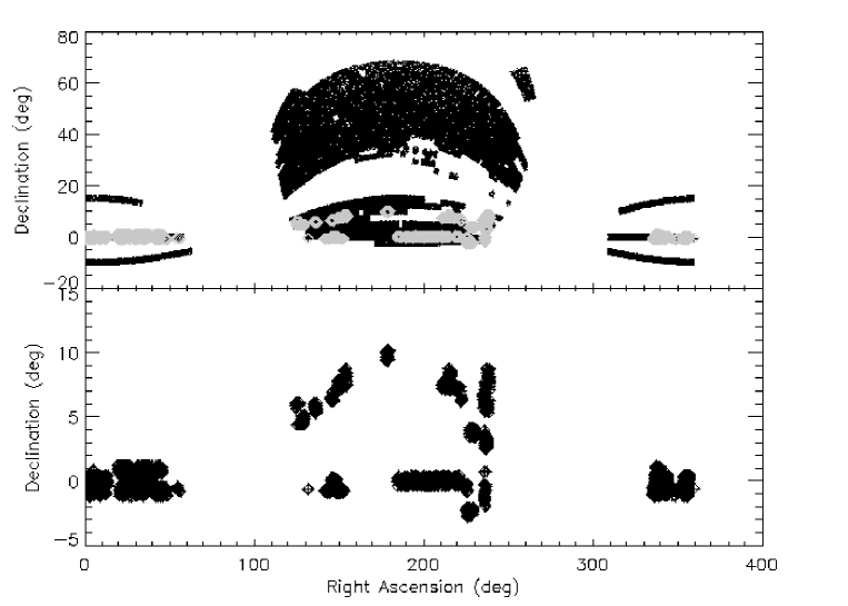
Figure 1: Positions of objects belonging to the three samples (see text). The upper figure represents the S-S sample while the lower shows the positions of the S-A sample members as black crosses and those of the S-UK sample members as grey diamonds.

The third sample (hereafter S-S) is composed by star-like sources belonging to the SDSS-DR5 ”Target” table and selected as candidate quasars according to the algorithm described in [Richards et al. 2002]. For all these objects spectroscopic classification (”specClass”) and redshifts are available. The only additional constraint applied to these objects is that their ”psf” magnitudes are required to be measured correctly in all photometric bands (using the photometric attribute ’flags’ contained in the PhotoObjAll table). The number of objects selected according to these requirements is 94196.

Table 1: Total number of members and ”specClass” distribution of the three samples.

Sample	Total	SP = 0	SP = 1	SP = 3	SP = 4	SP = 6
S-A	2719	43 (1.6%)	1176 (43.3%)	827 (30.4%)	73 (2.6%)	600 (22.0%)
S-UK	2159	23 (1.0%)	954 (43.5%)	773 (35.3%)	69 (3.1%)	373 (17.0%)
S-S	94197	2609 (2.4%)	22636 (20.4%)	53554 (48.4%)	4661 (4.2%)	10737 (9.67%)
S-SCat	158345	1782 (1.1%)	58801 (37.1%)	59052 (37.3%)	6332 (4%)	32360 (20.4%)

Figure 2: Redshift distribution for the three samples used in this work. S-A (dashed line) and S-UK (dotted line) samples counts have been multiplied by ten to increase their visibility.

In figures (1) and (2), we plot the positions and the redshift distribution for the members of the samples. The S-A and S-UK samples differ only for a few objects for which one or more UKIDSS magnitudes have not been measured and therefore their distributions in redshift space are almost identical. The distribution in redshift of S-S objects is characterized by a peak at $z\sim 1.7$. The composition of the different datasets described above in terms of the spectroscopic classification index ”specClass”, in addition to the composition of the dataset called ”S-SCat” used to extract the catalogue of photometric candidate QSOs described in paragraph (refSec:catalogues), are given in table (1).

3 Photometric selection of quasars

As a result of their distinct colours, the general idea behind all quasar candidate selection algorithms working in photometric parameter spaces is that quasars tend to lay far away from the regions occupied by normal stars (i.e. what is usually called stellar locus). Therefore, from the mathematical point of view, the problem of quasars candidate selection can be regarded as that of properly partitioning the parameter space in order to isolate the regions populated by quasars, minimizing the level of contamination from stars and the number of missed quasars. Spectroscopic observations of candidate quasars are crucial for quasars confirmation and to test the relative performances of the algorithm used to identify candidates. Such performances are usually expressed by two parameters, called respectively ”completeness $c$” and ”efficiency $e$”, and defined as follows:

$$c=\frac{\textsf{N candidates }}{\textsf{N \emph{a priori} known QSOs}};\ \ \ \ e=\frac{\textsf{N confirmed}}{\textsf{N candidates}}$$ (1)

It is apparent from the above definitions that $c$ provides a measure of how good is the method at retrieving all quasars in the sample, while $e$ provides a measure of the contamination in the list of candidates selected by the algorithm. In what follows we shall identify as ”base of knowledge” (BoK) the spectroscopically studied objects which can be used to build the samples of a priori known and ”confirmed” quasars. The optimal balance (if anything like that exists at all…) between completeness and efficiency is a delicate one since stars outnumber quasars by several orders of magnitude, and improving the efficiency by rejecting objects in regions of color space in which both stars and quasars are located, necessarily affects the completeness. Due to the unavoidable incompleteness in spectroscopic surveys (and as a matter of fact, of any other type of selection criterion), the BoK is always affected by biases which reflect into the value of $c$. In other words, in a given photometric catalogue, in order to have an exhaustive list of a priori known quasars, all objects should be observed spectroscopically and the same holds true for the list of candidates. The BoK is also needed to evaluate the errors. As an example, the knowledge of the intrinsic spread in quasar spectral indices translates into a lack of knowledge of the intrinsic spread in quasar colors [Richards et al. 2002]. The first attempt to produce a list of candidate quasars from multicolor survey data was by [Sandage & Wyndham 1965]. This pioneeristic attempt was soon followed by many others [Koo & Kron 1982, Schmidt & Green 1983, Warren & Hewett 1990, Warren et al. 1991], and more recently by [Hewett et al. 1995, Hall et al. 1996, Croom et al. 2001, Richards et al. 2002, Richards et al. 2004]. In what follows we shall shortly summarize two of them, focusing on those which have been tested on the SDSS data set and with whom our method will be compared.

3.1 Original SDSS selection algorithm

The official SDSS quasars candidate selection algorithm [Richards et al. 2002] (R02) is sensitive to quasars at all redshifts lower than $z\leq 5.8$ (i.e. very close to the theoretical limit predicted for the SDSS), and to atypical AGNs such as broad absorption line quasars and heavily reddened quasars. Performances of this algorithm, as stated in the paper, are a completeness $c\sim 90\%$ and an efficiency $e\sim 65\%$. The R02 algorithm under-samples certain regions of the colours space where degeneracy between colours of quasars in the redshift range $[2.2,3.0]$ arises. Since this redshift range is crucial for the cosmological applications which were the primary target of SDSS [Stoughton et al. 2002], objects falling in these regions were nonetheless selected paying the price of a worse overall efficiency.
Star-like objects are selected in a four dimensional colour space defined by the $(u,g,r,i,z)$ SDSS bands. Non stellar candidates are selected via their colours and by matching unresolved sources to the FIRST radio catalogues. The R02 algorithm can be summarised as follows: i) objects with spurious and/or problematic fluxes in the imaging data are rejected; ii) matches to unresolved FIRST radio sources are preferentially targeted without reference to their colors; iii) the sources remaining after the first step are compared to the distribution of normal stars and galaxies in two distinct three-dimensional colour spaces, one for low-redshift quasar candidates (based on the $ugri$ colors) and one for high-redshift quasar candidates (based on the $griz$ colours). The two groups are selected down to the limiting magnitudes $i^{*}\sim 19.1$ and $\sim 20.2$ respectively. Colour selection is performed accordingly to the their distance from a modelled, fixed hypersurface containing the stellar locus which, for a given photometric system, has been shown to be rather stable with respect to changes in stellar populations (e.g. [Richards et al. 2002]). No specific line is drawn between quasars and other types of active galactic nuclei. The completeness of the SDSS algorithm for QSOs candidate selection was also empirically measured by [Vanden Berk et al. 2005], using spectra of nearly 20,000 unresolved SDSS quasars to a reddening corrected magnitude of $i=19.1$. On the 278 $deg^{2}$ of the total area of the completeness survey, the combined colour and radio selection algorithms yield a completeness of $\sim 94.9^{+2.6}_{-3.8}\%$ at the $90\%$ confidence level. The completeness for the separate colour and radio selection algorithms are $\sim 93.8^{+2.6}_{-3.8}\%$ and $\sim 6.8^{+0.9}_{-0.9}\%$ respectively at the $90\%$ confidence level, leading to a higher estimate than the value reported by the R02 paper on a significantly larger sample of sources which have been spectroscopically observed.

3.2 Kernel Density Estimation-based QSO selection algorithm

The method for candidate QSOs selection discussed in [Richards et al. 2004] is based on the application of a nonparametric bayesian classification algorithm to evaluate the probability distribution function of different classes of sources inside the four dimensional SDSS photometric parameter space defined by the $(u,g,r,i,z)$ bands. The so-called kernel density estimation (hereafter KDE) algorithm is employed for the evaluation of the probabiliy density functions of stars and quasars distributions respectively, on a training set of labelled sources observed during the spectroscopic SDSS survey. After the training and test of the method, each photometric source is associated to the class of sources (stars or quasars) for which the estimated likelihood is higher. The performance of this method is expressed by an efficiency of 95.0% and a completeness of $\sim 90\%$ evaluated on the catalogue of unresolved UVX-excess candidates extracted from the DR1 SDSS photometric database. This method has been applied to the whole SDSS DR6 sample yielding a catalogue of about 1 million candidate QSOs [Richards et al. 2008], with a training set for QSOs comprising SDSS DR5 quasars dataset as listed by [Schneider et al. 2007], quasars discovered during the first observing season of the OAAOmega-UKIDSS-SDSS QSO survey, the whole high-redshift ($z>5.7$) sample of quasars discovered in SDSS data to date [Fan et al. 2006] and the 920 point sources selected as highly likely quasars from cross-comparison of SDSS and Spitzer data, according to two different mid-IR colour selections criteria [Lacy et al. 2004, Stern et al. 2005]. While the completeness is slightly smaller than the value measured using the first catalogue ($\sim 93.4\%$), the efficiency is almost unchanged, reaching an overall value of $\sim 95\%$.

4 Unsupervised quasar selection

Quasars candidates detection can be achieved using unsupervised clustering algorithms inside photometric colours space distribution of objects for which a reliable base of knowledge is available. The method presented in this paper follows a hierarchical approach which, starting from a preliminary clustering performed on the objects inside the parameter space, is followed by a second phase of agglomeration which reduces the initial number of clusters produced in the first step to an a priori unknown numbers of final clusters. We than have a phase which we shall call ”labelling”, based on the existing BoK, i.e. on the objects for which independent spectroscopic confirmation is available. This labelling is used to refine the partition of the parameter space in order to define the stellar and quasar loci. The characterization of the final clusters is then used to select ex novo the candidate QSOs.

The unsupervised clustering is accomplished using the Probabilistic Principal Surfaces algorithm which, strictly speaking is not a clustering algorithm but rather a nonlinear generalization of principal components particularly suited for dimensionality reduction purposes. As it will be shown, PPS project the input data onto a lower dimensionality space defined by what we shall call ’latent variables’ which act as attractors of input vectors and, therefore, can be interpreted as cluster centroids. The algorithm used for the second step is the so called Negative Entropy Clustering algorithm (hereafter NEC), which has been selected after comparative testing against other similar algorithms among the wide class of unsupervised hierarchical agglomerative clustering algorithms according to its high efficiency and reliability [Ciaramella 2005]. One advantage, which is as well a limitation, of this technique needs to be stressed: the distribution in the parameter space of the objects belonging to each cluster selected by the NEC is approximated by multivariate gaussians. Consequently, the projection of cluster members positions along each axis of the parameter space can be modelled as a one-dimensional gaussian, and common statistics quantities such as the average or the standard deviation can be used to describe the distribution of the members of each cluster over the entire parameter space. On the other hand, the assumption of gaussian shape for the clusters requires further discussion (see section (4.3)).

4.1 Latent variables and the PPS algorithm

The Probabilistic Principal Surfaces model [Chang 2000, Chang 2001, Staiano 2003] belongs to the family of the so called latent variables methods [Bishop 1999] and can be regarded as an extension of the Generative Topographic Mapping [Bishop 1998]. Since the one described here is the first application of this method to astrophysical issues, in what follows we shortly summarize the mathematical background, referring to the above quoted papers of a more detailed discussion. Uninterested readers may skip this paragraph and go directly to paragraph (4.2). The goal of any latent variable model is to express the distribution $p(\mathbf{t})$ of the variable $\mathbf{t}=(t_{1},\ldots,t_{D})\in\mathbb{R}^{D}$ in terms of a smaller number of latent variables $\mathbf{x}=(x_{1},\ldots,x_{Q})\in\mathbb{R}^{Q}$ where $Q<D$. In order to achieve it, the joint distribution $p(\mathbf{t},\mathbf{x})$ is decomposed into the product of the marginal distribution $p(\mathbf{x})$ of the latent variables and the conditional distribution $p(\mathbf{t}|\mathbf{x})$ of the data variables given the latent variables. It is convenient to express the conditional distribution as a factorization over the data variables, so that the joint distribution becomes:

$$p(\mathbf{t},\mathbf{x})=p(\mathbf{x})p(\mathbf{t}|\mathbf{x})=p(\mathbf{x})\prod_{d=1}^{D}p(t_{d}|\mathbf{x})$$ (2)

The conditional distribution $p(\mathbf{t}|\mathbf{x})$ is then expressed in terms of a mapping from latent variables to data variables, so that

$$\mathbf{t}=\mathbf{y}(\mathbf{x};\mathbf{w})+\mathbf{u}$$ (3)

where $\mathbf{y}(\mathbf{x};\mathbf{w})$ is a function of the latent variable $\mathbf{x}$ with parameters $\mathbf{w}$, and $\mathbf{u}$ is an $\mathbf{x}$-independent noise process. If the components of $\mathbf{u}$ are uncorrelated, the conditional distribution for $\mathbf{t}$ will factorize as in (2). From the geometrical point of view, the function $\mathbf{y}(\mathbf{x};\mathbf{w})$ defines a manifold in the data space given by the image of the latent space. The definition of the latent variable model needs to be completed by specifying the distribution $p(\mathbf{u})$, the mapping $\mathbf{y}(\mathbf{x};\mathbf{w})$, and the marginal distribution $p(\mathbf{x})$. The type of mapping $\mathbf{y}(\mathbf{x};\mathbf{w})$ determines the specific latent variable model. The desired model for the distribution $p(\mathbf{t})$ of the data is then obtained by marginalizing over the latent variables:

$$p(\mathbf{t})=\int p(\mathbf{t}|\mathbf{x})p(\mathbf{x})d\mathbf{x}.$$ (4)

This integration will, in general, be analytically intractable except for specific forms of the distributions $p(\mathbf{t}|\mathbf{x})$ and $p(\mathbf{x})$. PPS define a non-linear, parametric mapping $\mathbf{y}(\mathbf{x};\mathbf{W})$, where $\mathbf{y}$ is defined continuous and differentiable, which projects every point in the latent space to a point into the data space. Since the latent space is $Q$-dimensional, these points will be confined to a $Q$-dimensional manifold non-linearly embedded into the $D$-dimensional data space. This implies that data points projecting near a principal surface node (i.e., a Gaussian center of the mixture) have higher influences on that node than points projecting far away from it (cf. figure (3)). Each of these nodes $\mathbf{y}(\mathbf{x};\mathbf{w})$, $\mathbf{x}\in\{\mathbf{x}_{m}\}_{m=1}^{M}$ has covariance expressed by:

$$\mathbf{\Sigma}(\mathbf{x})=\frac{\alpha}{\beta}\sum_{q=1}^{Q}\mathbf{e}_{q}(\mathbf{x})\mathbf{e}_{q}^{T}(\mathbf{x})+\frac{(D-\alpha Q)}{\beta(D-Q)}\sum_{d=Q+1}^{D}\mathbf{e}_{d}(\mathbf{x})\mathbf{e}_{d}^{T}(\mathbf{x}),$$ (5)

$$0<\alpha<\frac{D}{Q}$$

where

• $\{\mathbf{e}_{q}(\mathbf{x})\}_{q=1}^{Q}$ is the set of orthonormal vectors tangential to the manifold at $\mathbf{y}(\mathbf{x};\mathbf{w})$,

• $\{\mathbf{e}_{d}(\mathbf{x})\}_{d=Q+1}^{D}$ is the set of orthonormal vectors orthogonal to the manifold in $\mathbf{y}(\mathbf{x};\mathbf{w})$.

The complete set of orthonormal vectors $\{\mathbf{e}_{d}(\mathbf{x})\}_{d=1}^{D}$ spans $\mathbb{R}^{D}$ and the parameter $\alpha$ is a clamping factor and determines the orientation of the covariance matrix. The unified PPS model reduces to GTM for $\alpha=1$ and to the manifold-aligned GTM for $\alpha>1$:

$$\mathbf{\Sigma}(\mathbf{x})=\left\{\begin{array}[]{ccc}0<\alpha<1&&\perp\mbox{to the manifold }\\ \alpha=1&&\mbox{$I_{D}$ or spherical }\\ 1<\alpha<D/Q&&\parallel\mbox{to the manifold. }\\ \end{array}\right.$$

In order to estimate the parameters $\mathbf{W}$ and $\beta$ we used the Expectation–Maximization (EM) algorithm [Dempster et al. 1977], while the clamping factor is fixed by the user and is assumed to be constant during the EM iterations. In a $3D$ latent space, then, a spherical manifold can be constructed using a PPS with nodes $\{\mathbf{x}_{m}\}_{m=1}^{M}$ arranged regularly on the surface of a sphere in $\mathbb{R}^{3}$ latent space, with the latent basis functions evenly distributed on the sphere at a lower density. The motivation behind such a spherical manifold is that spherical PPS are particularly well suited to capture the sparsity and periphery of data in large input spaces [Bishop 1995]. In order to better explain this issue let us consider the following low-D analogy first proposed by [Chang 2000]: … imagine fitting a rubber band ($2-D$ spherical manifold) to data distributed uniformly on the surface of a sphere in $\mathbb{R}^{3}$. Any fit bisecting the sphere into two equal halves will be optimal. On the other hand, consider using a piece of string to fit the same data. The string has a significantly lower probability of finding the optimal fit as it is open-ended… After a spherical PPS model is fitted to the data, the data themselves are projected into the latent space as points onto a sphere (figure (3)).

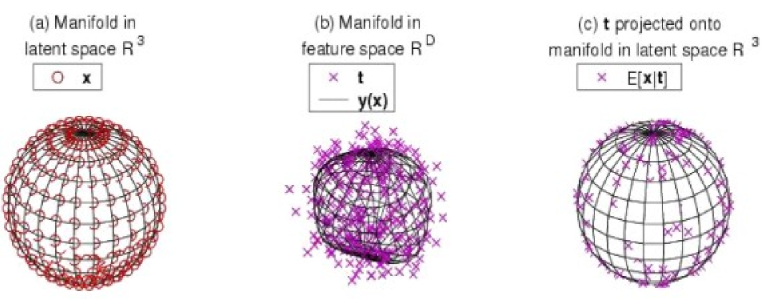
Figure 3: Schematic representation of the spherical manifold in the three dimensional latent space $R^{3}$ (a), the same manifold distorted in the feature space $R^{D}$ together with points associated to data (b), and the projection of the points distribution onto the surface of the spherical manifold embedded in $R^{3}$ latent space.

The latent manifold coordinates ${\mathbf{\hat{x}}}_{n}$ of each data point ${\mathbf{t}}_{n}$ are computed as:

$${\mathbf{\hat{x}}}_{n}\equiv\langle{\mathbf{x}}|{\mathbf{t}}_{n}\rangle=\int{\mathbf{x}}p({\mathbf{x}}|{\mathbf{t}})d{\mathbf{x}}=\sum_{m=1}^{M}r_{mn}{\mathbf{x}}_{m}$$

where $r_{mn}$ are the latent variable responsibilities defined as:

$${ll}r_{mn}=p(\mathbf{x}_{m}|\mathbf{t}_{n})= \frac{p(\mathbf{t}_{n}|\mathbf{x}_{m})P(\mathbf{x}_{m})}{\sum_{m\prime=1}^{M}p(\mathbf{t}_{n}|\mathbf{x}_{m\prime})P(\mathbf{x}_{m\prime})}$$ (6)

$$=\frac{p(\mathbf{t}_{n}|\mathbf{x}_{m})}{\sum_{m\prime=1}^{M}p(\mathbf{t}_{n}|\mathbf{x}_{m\prime})}$$ (7)

Since $\|\mathbf{x}_{m}\|=1$ and $\sum_{m}r_{mn}=1$, for $n=1,\ldots,N$, these coordinates lay within a unit sphere, i.e. $\|{\mathbf{\hat{x}}}_{n}\|\leq 1$. An interesting issue is the assessment of the incidence of each input data feature on the latent variables which helps to understand the relation between the features and the clusters found. The feature incidences are computed by evaluating the probability density of the input vector components with respect to each latent variable. More specifically, let $\{\mathbf{t}_{n}\}_{n=1}^{N}$ be the set of the D-dimensional input data, i.e $\mathbf{t}_{n}=(t_{n1},\ldots,t_{nD})\in\mathbb{R}^{D}$, and $\{\mathbf{x}_{m}\}_{m=1}^{M}$ be the set of latent variables with $\mathbf{x}_{m}\in\mathbb{R}^{3}$. For each data point $\mathbf{t}_{n}=(t_{n1},\ldots,t_{nD})$ we want to evaluate $p(t_{ni}/t_{n1},\ldots,t_{ni-1},t_{ni+1},\ldots,t_{nD},\mathbf{x}_{m})$, for $m=1,\ldots,M$ and $i=1,\ldots,D$. In detail:

$$p(t_{ni}/t_{n1},\ldots,t_{ni-1},t_{ni+1},\ldots,t_{nD},\mathbf{x}_{m})=$$ (8)

$$=\frac{p(t_{n1},t_{n2},\ldots,t_{nD},\mathbf{x}_{m})}{p(t_{n1},\ldots,t_{ni-1},t_{ni+1},\ldots,t_{nD},\mathbf{x}_{m})}=$$ (9)

$$=\frac{p(t_{n1},\ldots,t_{nD}/\mathbf{x}_{m})P(\mathbf{x}_{m})}{p(t_{n1},\ldots,t_{ni-1},t_{ni+1},\ldots,t_{nD}/\mathbf{x}_{m})P(\mathbf{x}_{m})}=$$ (10)

$$\frac{p(t_{n1},\ldots,t_{nD}/\mathbf{x}_{m})}{p(t_{n1},\ldots,t_{ni-1},y_{ni+1},\ldots,t_{nD}/\mathbf{x}_{m})}.$$ (11)

The last term is easily obtained since the numerator is simply the $m$-th Gaussian component of the mixture computed by the PPS model with mean $y(\mathbf{x}_{m};\mathbf{W})$ and oriented variance $\Sigma_{m}$, while the denominator is the same Gaussian component in which the $i$-th component is missing. Finally the mean of expression (8) over the $N$ input data points, for each $\mathbf{x}_{m}$, is computed. This explains why spherical PPS can be used as a ”reference manifold” for classifying high-D data. A reference spherical manifold is computed for each class during the training phase. In the test phase, a data previously unseen by the network is classified to the class of its nearest spherical manifold. Obviously, the concept of ”nearest” implies a distance computation between a data point $\mathbf{t}$ and the nodes of the manifold. Before doing this computation, the data point $\mathbf{t}$ must be linearly projected onto the manifold. Since a spherical manifold consists of square and triangular patches, each one defined by three or four manifold nodes, what is computed is an approximation of the distance. The PPS framework provides three approximation methods:

• Nearest Neighbour: finds the minimal square distance to all manifold nodes;

• Grid Projections: finds the shortest projection distance to a manifold grid;

• Nearest Triangulation: finds the nearest projection distance to the possible triangulation;

In what follows we used the Nearest Neighbour approximation method because it allows to evaluate distances of each data point in the feature space to all nodes embedded in the spherical manifold; even if computationally heavier than the other two methods, the Nearest Neighbour approximation provides the most trustworthy choice of the node (or nodes, in case of multiple nodes at the same distance from a given point) that each data point has to be assigned to. Another way to use PPS as classifiers consists in choosing the class $C$ with the maximum posterior class probability for a given new input $\mathbf{t}$. Formally speaking, let us suppose to have $N$ labelled data points $\{\mathbf{t}_{1},\ldots,\mathbf{t}_{N}\}$, with $\mathbf{t}_{i}\in\mathcal{R}^{D}$ and labels class in the set $\{1,\ldots,C\}$, then the posterior probabilities may be derived from the class-conditional density $p(\mathbf{t}|\emph{class})$ via the Bayes’ theorem:

$$P(\emph{class}|\mathbf{t})=\frac{p(\mathbf{t}|\emph{class})P(\emph{class})}{p(\mathbf{t})}\propto p(\mathbf{t}|\emph{class})P(\emph{class}).$$

In order to approximate the posterior probabilities $P(\emph{class}|\mathbf{t})$ we estimate $p(\mathbf{t}|\emph{class})$ and $P(\emph{class})$ from the training data. Finally, an input $\mathbf{t}$ is assigned to the class with maximum $P(class|\mathbf{t})$. In [Staiano 2003] and [Chang 2000] the effectiveness of PPS classifier is reported. A more detailed exposition of PPS as data mining framework can be found in [Staiano 2003, Staiano 2004]. We want to emphasise that the non-linear relation between the features and the latent variables evaluated by PPS cannot be expressed mathematically in a closed form since it is completely empirical in nature. A representation of this relation can be recovered observing the positions of the same groups of objects in both the original parameter space and in the latent space, after the projection onto the 2-dimensional surface embedded in the latent space (in this case, a spherical surface was chosen for the sake of clarity). In this way, it is possible to determine qualitatively the composition of latent variables, each associated to one and only one of the nodes of an equally-spaced grid overlaying the spherical surface, in terms of original data features. As an illustrative example of how the PPS algorithm works, a simplified experiment exploiting the S-A sample (see paragraph (2)) has been performed. The PPS algorithm has been applied to this sample after setting the number of latent variables to 14, so that 14 different pre-clusters were produced at the end of the process. Since this experiment is only aimed at showing the properties of the application of our algorithm to real data and does not pretend to identify any real clustering of the QSOs photometric parameter space, the initial resolution of the experiment was set to a smaller value than the one used for the real experiments (see paragraph (5)).

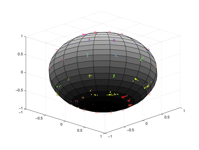
Figure 4: The distribution of points of S-A sample projected onto a spherical surface embedded into the latent space after PPS application. Each distinct pre-cluster produced by PPS algorithm from the original distribution of points into the parameter space is assigned a different colour and only points with confidence $p_{i}>0.8$ are shown. Arbitrary dimensions normalised to the radius of the sphere are shown on the three axes.

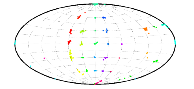
Figure 5: Aitoff projection of the distribution of points on the spherical surface embedded in the latent space as determined by PPS for the S-A sample of objects. In this figure, each distinct pre-cluster is assigned the same colour used in the previous plot, and only the points with confidence $p_{i}>0.8$ are drawn.

Figure (4) shows the pre-clusters produced by PPS inside the S-A sample and the projection of the members of this sample on the spherical surface embedded into the latent space. As already stated previously, each point in the initial parameter space is assigned to a unique pre-cluster according to the nearest latent variable; this proximity criterion is nonetheless applied only inside the latent variable space and does not necessarily translate on closeness of the corresponding projections of the points on the surface of the sphere. The final product of the PPS algorithm is a set of $N$ pre-clusters, whose $i$-th member $PC_{i}$ is formed by all closest points to the latent variable $LV_{i}$, which is associated to a node $N_{i}$ on the surface of the spherical surface. Only points having probability (also called confidence) $p_{i}$ to be assigned to the closest latent variable $LV_{i}$ greater than 0.8, have been plotted to make clearly visible the different regions of the spherical surface, and as a consequence, of the latent space occupied by different pre-clusters. Each pre-cluster has been plotted with a different colour, which has been used throughout the plots to label the same pre-cluster. Figure (5) shows the Aitoff projection of the same pre-clusters produced by PPS. In order to prevent from misleading interpretations of figures (4) and (5), it is worth noticing that the number of nodes appearing on both the spherical surface and its Aitoff projection is greater than the actual number of latent variables used for the experiment. The grid is used only to ease the comprehension of the distribution of pre-clusters. The composition of the latent variables responsible for each pre-cluster in terms of the original features of the parameter space is shown in figure (6), where points belonging to the same pre-clusters are drawn in the planes obtained by projecting the original parameter space distribution onto some of the possible couples of parameters, using the same colour code used in both plots (4) and (5). A qualitative guess of the composition of each latent variable found by PPS in terms of the variables of the original parameter space is possible comparing the positions of the members of each pre-cluster in the original parameter space and in the latent space. As it can be seen in figure (6), the method is much more effective than the classical clustering algorithms in disentangling groups of objects which appear indistinguishable in the simple colour-colour diagrams. Except for few clusters placed at the extremes of the nearly one-dimensional locus visible in ($g-r$) vs ($r-i$) and ($r-i$) vs ($i-z$) plots, all the other clusters appear to be almost inextricably mixed, so that discriminating them even on the bases of an unusual partition of these planes appears to be impossible.

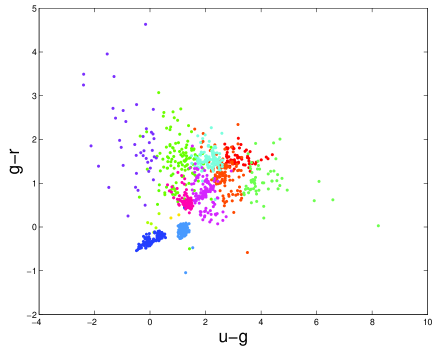
(a) ($u-g$) vs ($g-r$)

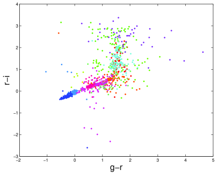
(b) ($g-r$) vs ($r-i$)

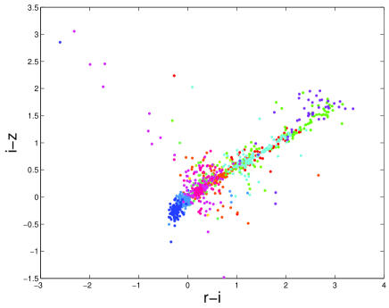
(c) ($r-i$) vs ($i-z$)

Figure 6: Original parameter space distribution projected on three planes of the members of sample S-A after the application on the PPS algorithm. Different pre-clusters are drawn with different colours following the same colour-scheme used in figures (4) and (5). In all these figures, only the points with confidence $p_{i}>0.8$ are drawn.

4.2 PPS as a clustering tool

It needs to be explicitly noted that, as already mentioned, even though strictly speaking PPS are not a clustering algorithm, they can be effectively used for clustering purposes. Each latent variable, in fact, defines an attractor for points which are projected near to it and therefore the input space is partitioned in a number of clusters coinciding with the number of latent variables. The number of latent variables can therefore be regarded as the initial ’resolution’ of clustering process but, provided that this number is not too low or too high (to avoid respectively a rough and unspecific or sparse clustering), it is found empirically that every reasonable choice leads to consistent results. In fact it suffices to set it to a higher value than the number of clusters realistically expected to appear in the data and then to use an agglomerative algorithm capable of recombining clusters of points artificially split into two or more chunks of smaller size. In our case we used the Negative Entropy Clustering described in the following paragraph.

4.3 The hierarchical clustering algorithm

Most unsupervised methods require the number of clusters to be provided a priori. This circumstance represents a serious problem when exploring large complex data sets where the number of clusters can be very high or, in any case, largely unpredictable. A simple threshold criterion is not satisfactory in most astronomical applications due to the high degeneracy and noisiness of the data which can often lead to an erroneous agglomeration. A classical agglomerative clustering algorithm is completely specified by assigning a definition of distance between clusters and a linkage strategy, i.e. a rule according to which clusters separated up to a given value of the distance are merged and others are not. Several definitions of distances can be found in the literature (distance between centroids of the clusters, maximum distance between members of the clusters, minimum distance, etc.) and many linkage strategies are used for common tasks (for example simple linkage, average, complete, Ward’s, etc.). Independently from the choice of the distance definition, successive generations of merging are carried out using updated distances between clusters: the resulting structure of clusters can be represented by a tree-like graph, called dendrogram (see below for more details) until some convergence or threshold criterion is satisfied (so that, at the end of the process, there are no clusters to be merged). A strictly geometrical interpretation of distances between clusters in the parameter space can be relaxed in order to generalise this class of algorithm. In this framework, the distance between clusters is a generic function of the composition of the clusters in terms of parameter space coordinates. We chose an approach to the hierarchical clustering based on the combination of a similarity criterion founded on the notion of ’Negative Entropy’ and the use of a dendrogram to investigate the structure of clusters produced during the agglomerative process. We made use of the Fisher’s linear discriminant which is a classification method that first projects high-dimensional data onto a line, and then performs a classification in the projected one-dimensional space [Bishop 1995]. The projection is performed in such a way to maximize the distance between the means of the two classes while minimizing the variance within each class. At the same time, the differential entropy H of a random vector is defined as:

$${\mathbf{y}}=(y_{1},\ldots,y_{n})^{T}$$

with density $f({\mathbf{y}})$:

$$H({\mathbf{y}})=\int f({\mathbf{y}})\log f({\mathbf{y}})d{\mathbf{y}}$$

so that negentropy $J$ can be defined as:

$$J(\mathbf{y})=J({\mathbf{y}}_{Gauss})-H(\mathbf{y})$$

where $\mathbf{y}_{Gauss}$ is a Gaussian random vector of the same covariance matrix as $\mathbf{y}$. The Negentropy can be interpreted as a measure of non-Gaussianity and, since it is invariant for invertible linear transformations, it is obvious that finding an invertible transformation that minimizes the mutual information is roughly equivalent at finding directions in which the Negentropy is maximised. Our implementation of the method uses an approximation of Negentropy that provides a good compromise between the properties of the two classic non-Gaussianity measures given by Kurtosis and Negentropy. Negentropy clustering algorithm can be used to perform unsupervised agglomeration of pre-clusters found by the PPS algorithm during the first step of our method. The only a priori information needed by NEC is a particular scalar value of the Negentropy called dissimilarity threshold $T$. We suppose to have $n$ $D$-dimensional preclusters $X_{i}$ with $i=1,\ldots,n$ that have been determined by the PPS; these clusters are passed to the Negentropy Clustering algorithm which, in practice, ascertains whether each couple of contiguous clusters (according to the Fisher’s linear discriminant) can or cannot be more efficiently modelled by one single multivariate gaussian distribution. In other words, NEC algorithm determines if two clusters belonging to a given couple can be considered to be substantially distinct or parts of a greater more general data set (i.e. cluster). This method can be easily generalized to other model distributions; we preferred to use a multivariate gaussian model only because the normal distribution can be considered a good approximation of any reasonably shaped peaked distribution, since the colours of objects belonging to the same observational family of QSOs are widespread around a central value due to several physical mechanism (differential scattering, absorption, etc.) and observational effects. Similarly to what was done for the PPS algorithm, in order to elucidate the interpretation of the results from this unsupervised agglomerative method, we used NEC to generate a set of final clusters from the pre-clusters produced by the PPS algorithm inside the S-A sample already used in the illustrative example described in paragraph (4.1). The pre-clusters underwent the clustering process displayed in the figure (7) in the form of a dendrogram, i. e. a tree-diagram frequently used to illustrate the arrangement of the clusters produced by agglomerative or divisive algorithms. This kind of representation of a clustering process consists of many U-shaped lines connecting objects in a hierarchical tree: the height of each U represents the value of a distance function evaluated between the two objects being connected; the distance definition depends on the specific kind of clustering algorithm considered. In our case, the quantity reported on the vertical axes is the negative entropy, a measure of the non-gaussianity of the multivariate distribution obtained merging the couple of clusters connected by the branches of the U-shaped lines. The optimal set of clusters (in a sense that will be stated clearly in paragraph (4.4)) is obtained for a certain value of negentropy, called the critical value of the dissimilarity threshold $T=T_{cr}$. In the illustrative experiment considered in paragraph (4.1), only points with confidence greater than 0.8 were retained for clustering, so that the final number of clusters is equal to 3, corresponding to the critical dissimilarity threshold $T_{cr}=1.46$. The composition of these clusters in terms of individual points of the S-A sample and of the pre-clusters which have been passed to the NEC algorithm, is showed in figure (8), where the positions of points in the 4 dimensional original parameter space are projected onto the same colour-colour planes used in figure (6).

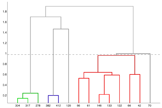
Figure 7: An example of dendrogram (see text for details) used as a representation of an agglomerative clustering process performed by the NEC algorithm. On the x and y axes are respectively reported the numeric labels of the initial clusters and the values of the dissimilarity threshold. The dashed line intersects the lines of the tree-like graph associated with the clusters produced by the clustering process when the value of the dissimilarity threshold has been fixed to $T_{cr}=1$.

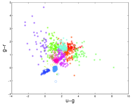
(a) (u - g) vs (g - r)

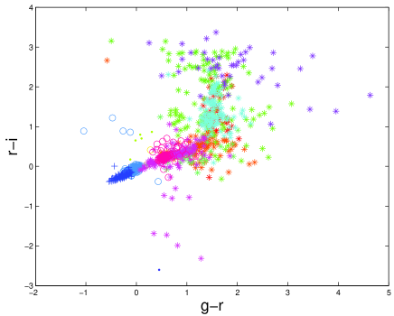
(b) (g - r) vs (r - i)

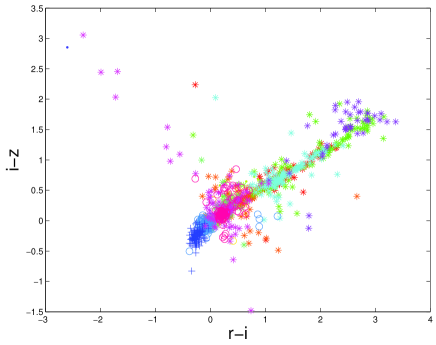
(c) (r - i) vs (i - z)

Figure 8: Original parameter space distribution projected on three colour-colour planes of the members of sample S-A after the application of the Negative Entropy Clustering algorithm to the pre-clusters produced by PPS. Former pre-clusters are drawn with different colours following the same colour-scheme used in figures (4) and (5). Each final cluster is separated and singled out over the pre-clusters distribution through different marker symbols.

Colours and marker shapes of each point are respectively associated to the pre-cluster and final cluster membership of the objects, so that becomes feasible the analysis of the relationship between the input and output of NEC algorithm in terms of the original distribution of points inside the parameter space and the pre-clusters used as input of the clustering algorithm. The three figures in (8) show that the cluster whose members are marked as crosses appears to be isolated in the first plot and clearly distinguishable from the other two in the remaining colour-colour plots, while the clusters represented by circles and asterisks are entwined in all the plots and their members can be barely discriminated.

4.4 The labelling phase

The results of the agglomeration performed by the NEC algorithm depend crucially on the value of the dissimilarity threshold $T$. Since different clustering processes of the data set correspond to different values of this constant, it is necessary to apply an objective criterion for the determination of the best (hereafter critical) value of the dissimilarity threshold $T_{cr}$, i.e the value leading the best performance in terms of the selection algorithm completeness and efficiency. To this aim, we use the BoK to label as ”goal-successful” those clusters $C_{j}$ (with $j\in\{1,...,N_{cl}\}$ (where $N_{cl}$ is the total number of clusters for a given value of $T$), for which the following relation is satisfied:

$$sr_{j}^{(g)}=\frac{\textsf{Nm confirmed "goal" members in }C_{j}}{\textsf{Nm members in }C_{j}}\geq\widetilde{sr}^{(g)}$$ (12)

i.e., the fraction $sr^{(g)}$ of ”goal” objects contained in the cluster $C_{j}$ must be higher then a given value $\widetilde{sr}^{(g)}$. At the same time ”notgoal-successful” clusters are defined as clusters for which the following relation holds:

$$sr_{j}^{(ng)}=\frac{\textsf{Nm confirmed "notgoal" members in }C_{j}}{\textsf{Nm members in }C_{j}}\geq\widetilde{sr}^{(ng)}$$ (13)

with a similar meaning of the symbols. In other words, ”goal-successful” (”notgoal-successful”) clusters are defined as the clusters containing ”goal” (”notgoal”) objects fractions above a given threshold. A third type of clusters which we shall simply call ”not successful” are those which do not fulfill any of the two above definitions as they are formed by comparable fractions of ”goal” and ”notgoal” objects. In the specific case addressed here, they will be composed by a mixture of confirmed quasar and other types of objects (mainly stars). The critical value $T_{cr}$ of the dissimilarity threshold is therefore defined as the one which, given a set of initial clusters provided by the PPS algorithm, produces the maximum number of ”goal-successful” clusters, or, in a more quantitative fashion, as the value which maximizes the normalised success ratio NSR:

$$NSR(T)=\frac{\textsf{Nm successful clusters}}{\textsf{Nm clusters}}$$ (14)

A further requirement is imposed to select $T_{cr}$ is that the number of clusters produced has to range between 25 $\%$ and 75 $\%$ of the number of initial clusters. This last constraint excludes from the selection values of $T_{cr}$ producing unreasonable numbers of clusters, namely an excessive number of poor clusters or few very reach clusters (for a detailed discussion see section (6.3)), even if this requirement has been loosened during each experiment in order to check if any feasible clustering combination had been dropped. The process described hitherto is recursive: once $\widetilde{sr}^{(g)}$ and $\widetilde{sr}^{(ng)}$ have been fixed, the suitable value of the dissimilarity threshold is identified and a first clustering is performed using $T_{cr}$ as an imput to the NEC algorithm. All successful clusters produced in this first generation of clustering are ’frozen’ and the efficiency $e_{1}$ is estimated; unsuccessful clusters are merged, forming the input data set for the following iteration of the selection process. After this second iteration, the new ”goal-successful” and ”notgoal-successful” clusters, if any, are retrieved and stored. The procedure is repeated until no other successful clusters are determined. Critical values of the dissimilarity threshold for each generation are fixed according to the same criteria explained above. The total efficiency $e_{tot}$ of the selection is defined as the sum of the efficiencies of each of $M$ generations weighted according to the total number of objects belonging to the ”goal-successful” clusters of that generation:

$$e_{tot}=\frac{\sum_{i=1}^{M}n_{i}e_{i}}{\sum_{i=1}^{M}n_{i}}=\frac{\sum_{i=1}^{M}n_{i}^{(goal)}}{N_{tot}^{(goal)}}\ \ \ \ \$$ (15)

where $n_{i}$ is the total number of objects belonging to ”goal-successful” clusters of the $i_{th}$ generation such that $\sum_{i=0}^{M}n_{i}=N_{tot}^{(goal)}$ and $n_{i}^{(goal)}$ is the number of confirmed goal objects contained in all ”goal-successful” clusters selected in the $i$-th generation.

The total completeness $c_{tot}$ of the process is similarly defined:

$$c_{tot}=\frac{\sum_{i=1}^{M}n_{i}^{(goal)}}{N_{tot}^{(all)}}$$ (16)

where $N_{tot}^{(all)}$ is total number of goal objects contained in the data set used for the experiment. Extensive testing showed that, within the range $\left[0.65,0.90\right]$ the values of the constant thresholds $\widetilde{sr}^{(g)}$ and $\widetilde{sr}^{(ng)}$ for ”goal-successful” and ”notgoal-successful” clusters respectively, do not affect the final efficiency and completeness of the method but only the number of generations of the process needed to achieve the final result. The selection performances of the labelling phases are estimated for all the experiments described in this paper as functions of one of the parameters used for the clustering and the redshift of the members of the data set considered, using the available BoK to measure the local values of efficiency and completeness in the resulting redshift vs parameter plane. As an example, in the upper left-hand panel and right-hand panel of figure (9) are shown respectively the efficiency $e$ and the completeness $c$ in the redshift vs ($u-g$) plane of the illustrative experiment discussed in the previous sections. The colours of the cells are associated to the normalized values of efficiency and completeness expressed by the colourbars visible on the right of the plots. In the plots of the efficiency, each cell contains the total number of candidates selected by the algorithm in that region of the plane (the number of confirmed candidate being the product of this number by the efficiency in the cell), while in the plots showing the local values of completeness the numbers represent the amount of confirmed QSOs according to the BoK (the number of confirmed objects selected being the product of this number by the completeness in the cell). Blank cells represent regions of the plane where no candidate belonging to the BoK is found. The lower panels of figure (9) contain respectively a graphical representation of the partition of the redshift vs ($u-g$) plane in terms not only of the ”goal-successful” clusters used for candidate selection, but also in terms of the other two types of clusters produced by our algorithm, namely the ”notgoal-successful” and ”unsuccessful” ones. Each cell containing at least one object belonging to the reference catalogue is marked with a different symbol according to the type of the cluster (circles for ”goal-successful”, crosses for ”notgoal-successful” and asterisks for ”unsuccessful” clusters) contributing the higher efficiency to the selection of QSOs candidates in that region of the plane. Also in this case, the colours of the cells represent the maximum values of efficiency and completeness respectively.

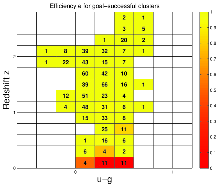
(a) Efficiency in $z$ vs $u-g$ plane (”goal-successful”)

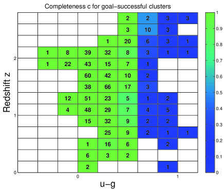
(b) Completeness in $z$ vs $u-g$ plane (”goal-successful”)

Figure 9: Efficiency (left-hand panel) and completeness (right-hand panel) in the redshift vs ($u-g$) plane for the labelling phase of the illustrative experiment. Colour of the cell is associated to the efficiency and completeness of the selection process of the ”goal-successful” clusters, while the numbers contained in each cell represent the total number of candidates in that region of the $z$ vs $u-g$ plane.

4.5 Selection of candidate quasars from photometric samples.

After the labelling phase, which provides the most suitable partition of the parameter space in terms of selection of ”goal-successful” and ”notgoal-successful” clusters, candidate quasars extraction from a purely photometric data set (i.e., for which no spectroscopic BoK is available) can be carried out using one of the three different approaches explained in the following paragraphs.

4.5.1 Method I: ”re-labelling”

The first method, hereby called ”re-labelling”, is based on the assumption that confirmed QSOs in the BoK are tracers of successful clusters containing mainly goal objects even when other objects are added to the sample. The data-set used for the labelling and the photometric sample are merged and the whole process described in the previous paragraphs is repeated using this extended group of objects. The selection of candidate quasars is then carried out considering as candidates all non-BoK objects belonging to clusters where spectroscopic confirmed quasars (membersof the sample used for the labelling) are dominant. This simple and, at least in theory, straightforward method unfortunately is applicable only when the non-BoK sample is composed by few objects, namely a small fraction of the number of BoK objects. The reason is that PPS algorithm determines the best projection from the parameter space to the latent space by modelling a probability distribution which is a function of the initial distribution of BoK sample objects inside the initial space. New objects added to the labelling sample modify the shape of the probability density function and the final result of the unsupervised clustering, so that the efficiency and completeness estimated during the labelling phase are not appropriate. It is worthwhile to emphasize that this method has to be preferred when limited amount of data are added to an existing data set but that it cannot be used when the amount of new data to be processed is large.

4.5.2 Method II: colours cuts

The second approach at the extraction of candidate QSOs from the photometric dataset is based on the geometrical characterization of the distribution of the sources belonging to the ”goal-successful” clusters in the parameter space. In general, for any ”goal-successful” cluster in a $n$-dimensional parameter space, 2$n$ constraints are identified as some values of statistical meaning associated to the distribution of points of the cluster along each axis of the parameter space. The candidate objects are selected applying to the photometric data set the cuts derived by the 2$n$ generic constraints as the objects which satisfy these requirements. This method is more flexible than the previous one since the selection of candidate QSOs can be fine-tuned by modifying the cuts applied to the parameters in order to achieve different performance goals. Obviously, this choice yields a trade-off between efficiency and completeness of the selection. For instance, loose constraints allow to select a larger number of candidates in the outskirts of the clusters, where the contamination from ”notgoal” sources is higher, thus resulting in a increased completeness but in a lower efficiency of the overall selection process. On the other hand, tight constraints increase the efficiency of the algorithm at the cost of a lower completeness, by selecting only the central regions of the parameter space occupied by successful clusters. In the present work two different prescriptions have been used to determine the cuts in the parameter space. According to the first prescription, $n$-haedrons whose vertices are set by the extremal values of cluster members distribution for each parameter for both ”goal-successful” and ”notgoal-successful” clusters, were chosen to establish the regions of the parameter space containing candidate quasars. More precisely, all photometric objects found inside the $n$-haedrons containing ”goal-successful” clusters and not selected by any of the $n$-haedrons derived by ”notgoal-successful” clusters are selected as candidate quasars. Errors on parameters have been used to estimate the distance of each object from the surfaces of the $n$-haedrons generated by ”goal-successful” clusters, in order to avoid the possible contamination from spurious objects placed near to the borders of the ”goal-successful” regions. More precisely, only inner objects with distance from the surfaces of the ”goal-successful” $n$-haedrons larger than 3$\sigma$ have been retained as candidates. The second prescription is more conservative (in the sense of ensuring higher efficiency and lower completeness) than the first one: in order to reduce the fraction of contaminants, the vertices of the $n$-haedrons describing the positions of ”notgoal-successful” clusters are set to the positions $\bar{x}_{i}\pm\sigma_{i}$ along each axis of the parameter space, where $\bar{x}_{i}$ is the average value and $\sigma_{i}$ the standard deviation of the distribution of points along the $i$-th axis. All objects placed inside these $n$-haedrons are discarded and the remaining are selected as candidate according to the first prescription.

4.5.3 Method III: Mahalanobis’ distance

The third method for the extraction of photometric candidate objects is based on the notion of Mahalanobis’ distance. This particular type of distance differs from the euclidean one since it takes the dispersion of the each variable and correlations among multiple variables into account when determining the distance between two points. In general, given two generic points $\vec{x}=(x_{1},...,x_{p})^{t}$ and $\vec{y}=(y_{1},...,y_{p})^{t}$ in the $t$-dimensional space $R^{t}$, the Mahalanobis’ distance between them is defined as:

$$d_{S}=\sqrt{(}(\vec{x}-\vec{y})^{t}S^{-1}(\vec{x}-\vec{y}))$$ (17)

where $S^{-1}$ is the covariance matrix. Mahalanobis’ distance is widely employed in cluster analysis and other classification techniques, since it is possible to use it to classify a test point as belonging to one of a set of more clusters defined in the same space where the test point resides. The first step is the estimation of the covariance matrix of the clusters, usually achieved through a set of realizations of the populations of each clusters represented by samples of points drawn from the same statistical distribution. Then, given a test point, Mahalanobis’ distances $d_{Mal}$ of this point from all clusters are calculated and the point is assigned at that cluster for which $d_{Mal}$ is the smallest. In the probabilistic interpretation given above, this is equivalent to selecting the class to which is more probable that the given point belongs. In this work, given a set of clusters produced by the combined PPS and NEC algorithms, Mahalanobis’ distance has been used to assign each member of the photometric data set to the its nearest cluster. Only objects associated to ”goal-successful” clusters have been considered QSOs candidates. An interesting consideration about this method can be made by recalling that the usage of Mahalanobis’ distance to evaluate the membership of objects to a given set of ”goal-successful” clusters with a threshold value (a maximum distance beyond which an object is not assigned to any clusters) can be exploited to select outliers or rare objects were not included in the BoK because of their scarcity.

4.6 Comparison of the photometric candidate selection methods

In order to compare the performances of the methods described in the previous paragraphs, we used instead of the set of clusters produced by the illustrative experiment described in paragraphs (4.1) and (4.3), the set of clusters produced in the first experiment (see paragraph (5.1)) since our goal, in this case, is to evaluate the best method of photometric candidate selection in terms of the clusters labelling produced in a real scientific application of the method. First of all, it is worthwhile to remind the reader that the ”re-labelling” method can be effectively used only in case the number of photometric objects is much smaller than the number of objects composing the base of knowledge (i.e., the objects whose clustering in the parameter space has been determined, c.f. paragraph (4.5.1)). In addition, this approach is very time-consuming since a whole new application of PPS and NEC algorithms is needed every time that a new sample of photometric sources is considered, even if the BoK remains unchanged. For these reasons, this method though theoretically interesting is not well suited for large scale data sets and will not be further considered in the following comparison. The other two methods have been compared by applying both of them to the same sample of objects randomly drawn from the S-A sample used for the first phase of the experiment. Only the original parameters associated to these objects, namely the four colours derived from the optical magnitudes measured in SDSS $(u,g,r,i,z)$ photometric system, were used for the selection. The total performances, in terms of efficiency $e$ and completeness $c$, evaluated for the ”re-labelling”, Mahalanobis’ distance and the ”colours cuts” methods (with the two different prescriptions described in (4.5.2)) on the ”goal-successful” clusters produced by the first experiment are shown in the table (2), exploiting the BoK associated to the S-A sample. A more detailed comparison of the performances of the two methods considered for the selection of photometric candidates is shown in figures (10), where the two indicators are plotted as functions of the redshift and of one of the photometric parameters, namely the $u-g$ colour of the source (the choice of the particular colour is not important in this case since the methods of selection show similar relative performances when other colours are considered). Each cell in the redshift vs colour plane is coloured according to the local value of efficiency and completeness as specified by the colourbar, while the integers written inside the cells represent the numbers of candidates selected by the algorithm and confirmed QSOs according to the BoK for efficiency and completeness plots, respectively (for details, see section (4.4)).

Method	$e$	$c$
Re-labelling (few photo objects)	81.3%	89.4%
Colours cuts (1st prescription)	79.8%	87.6%
Colours cuts (2nd prescription)	81.1%	79.4%
Mahalonobis’ distance	81.0%	88.8%

Table 2: Efficiency and completeness calculated for three methods of selection of photometric candidates using the clusters labelling obtained in the first experiment.

The comparison of the upper and lower panels in figure (10) clearly shows that the Mahalanobis’ distance method offers higher efficiency and completeness in large swaths of the redshift vs ($u-g$) plane than the colours cuts method, improving in particular the completeness of the selection in the redshift range $[1,2]$. Since the best method in terms of both local and total efficiency and completeness is the Mahalanobis’ distance, it has been used for the extraction of the lists of QSOs photometric candidates (for details see paragraph (8)) determined on the bases of the experiments described in this paper.

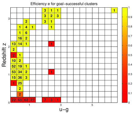
(a) Efficiency $e$ for the second method in $z$ vs $u-g$ plane

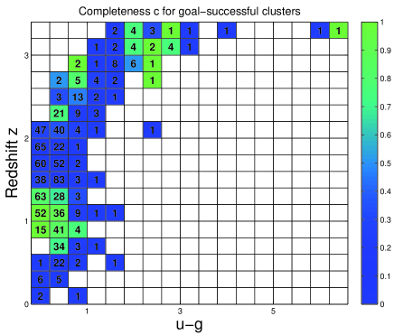
(b) Completeness $c$ for the second method in $z$ vs $u-g$ plane

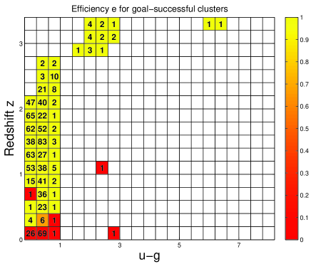
(c) Efficiency $e$ for the third method in $z$ vs $u-g$ plane

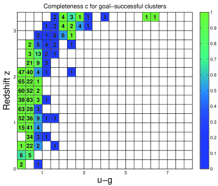
(d) Completeness $c$ for the third method in $z$ vs $u-g$ plane

Figure 10: Efficiency (left-hand panel) and completeness (right-hand panel) in the redshift vs $u-g$ plane for the colours cuts (upper panels) and Mahalanobis’ distance (lower panels) methods of photometric candidates selection. Colours of the cells express the local values of efficiency and completeness while integers represent the numbers of candidates selected by the algorithm and confirmed QSOs according to the BoK for efficiency and completeness plots respectively.

5 The experiments

Four different sets of experiments based the samples labelled from 1 to 4 and described above have been performed in order to evaluate the ability of the method to select candidate QSOs using different BoKs (although based on the same ”specClass” index from the SDSS) in different photometric parameter spaces. The following are the set-up of the four experiments:

• The first experiment is based on the S-A sample, composed by all SDSS star-like objects for which a spectroscopic classification is available and falling into the region of overlap with the UKIDSS-DR1 LAS. Colours have been calculated using optical ”psf” magnitudes to define the parameter space where the clustering is carried out.

• The second and third sets of experiments exploit the S-UK sample, i. e. all stellar objects in the SDSS having spectroscopic classification and matching with a stellar NIR counterpart belonging to the UKIDSS-DR1 LAS catalogue. We made use of optical plus infrared colours only (second experiment) and only optical colours (third experiment).

• The fourth set of experiments explored the distribution of S-S data set (formed by all candidate QSOs in SDSS-DR5 according to the official Sloan selection algorithm for which all 5 ”psf” magnitudes were correctly measured) inside the photometric parameter space determined by their optical colours.

Table 3: Total efficiency and completeness of the experiments.

Experiment	Sample	$e_{tot}$	$c_{tot}$	$n_{gen}$
1	S-A	81.5%	89.3%	2
2	S-UK	92.3%	91.4%	1
3	S-UK	97.3%	94.3%	1
4	S-S	95.4%	94.7%	3

The colours used for all these experiments were calculated using adjacent bands: $u-g$, $g-r$, $r-i$, $i-z$ for the optical bands, and $Y-J$, $J-H$, $H-K$ for the near infrared ones. The dependance of the results on the choice of the colours will be discussed in section (6). The final results of these experiments in terms of total efficiency and completeness of the candidate quasars selection are summarised in table (3) while the number of successful clusters and the fraction of confirmed quasars and stars inside each ”goal-successful” cluster for each experiment are reported in table (4). A colour-colour plot is shown for each experiment for the comparison of the results of the candidate selection method exposed in this paper with the classical colour-colour selection techniques commonly employed in the astronomical literature. At the same time, plots of the local values of the efficiency and completeness in the redshift vs ($u-g$) plane are displayed for each experiment and will be discussed in section (8). The same plots for all the others colours for each experiment are shown in the appendix (A).

5.1 First experiment

This experiment is aimed at comparing the SDSS native selection algorithm to our method. The number of latent variables (i.e. initial clusters) used for the PPS pre-clustering was 62, and the critical value of the dissimilarity threshold was chosen according to the criteria explained above. The normalised success ratio and other statistical indicators of the clustering process are plotted as functions of the dissimilarity threshold in the upper left-hand panel of figure (11). The estimated efficiency and completeness of the selection process are shown in the upper right-hand panel of figure (11) as functions of the dissimilarity threshold as well. The distribution of sources as a function of redshift and spectroscopic classification ”specClass” in the ”goal-successful” clusters selected in this experiment is shown in the lower left-hand panel of figure (11) while, a ”box and whisker” plot of the distribution of candidate QSOs for each ”goal-successful” cluster selected in this experiment is shown in remaining panel of figure (11).

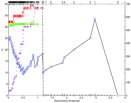
(a) NEC diagnostics

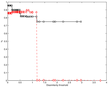
(b) Efficiency and completeness

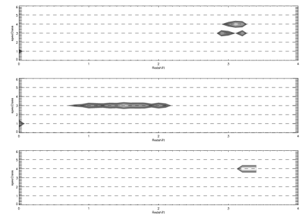
(c) specClass vs redshift plane distribution of clusters

(d) ”Box and wisker” plot of clusters

Figure 11: Upper left-hand panel: In this figure, the fraction of ’goal-successful’ clusters (squares), the total percentage of all sources objects belonging to ’goal-successful’ clusters (circles), the total percentage of objects belonging to ’goal-successful’ clusters irrespective of their spectroscopic classification (diamonds) and variance of ’goal-successful’ clusters (asterisks) are plotted as a function of the dissimilarity threshold for the first experiment. Upper right-hand panel: total estimated efficiency $e_{tot}$ (square symbols) and completeness $c_{tot}$ (diamond symbols) of the candidate quasars selection process as functions of the dissimilarity threshold for the first experiment. Lower left-hand panel: distribution of members of ”goal-successful” clusters in the first experiment in the specClass-redshift plane. Lower right-hand panel: ”box and whisker” plot of the distribution of different clusters produced in the first experiment. The black rectangle indicates the 95% confidence interval for the median while the greater rectangle is contained between the first and third interquartile. The notches extend to $\pm 1.58$ of the interquartile range times the inverse of the square root of the number of objects. Outliers are represented as dots.

The three ”goal-successful” clusters selected in this experiment are evenly distributed in terms of colours:

• The first cluster is formed by objects having $u-g$ ranging form 2.0 to 2.5 and the other colours averaging between 0.5 and 0 with little dispersions. These objects have redshift around 3 and they are mainly classified as high-redshift QSOs in terms of spectroscopic ”specClass” classification, with a little contamination by misidentified stars (”specClass” = 1).

• The second cluster contains the vast majority of objects and is mainly formed by normal QSOs (”specClass” = 3), with redshift ranging from 0.8 to 2.0, except for a little fraction of stars. In terms of colours distribution, this cluster shows all colours having average values near 0.0 with a higher and asymmetric dispersion, caused by outliers mainly having higher colours values than the average.

• The third ”goal-successful” cluster members are characterized by a very high $u-g$ values, compared to the average values of the others colours which are similar to those found for the first cluster. It is formed by only high redshift ($z>3$) QSOs with spectroscopic classification ”specClass” = 4.

The distribution of objects in the ($u-g$) vs ($g-r$) plane and belonging to the ”goal-successful” clusters selected during the first experiment is shown in the figure (13). A combined colour and symbol code has been used: confirmed QSOs according to the BoK are drawn using a cross symbol, while objects which the BoK identifies as confirmed not QSOs are drawn as circles. On the other hand, all the points belonging to ”notgoal-successful” and ”unsuccessful” clusters are painted using black and grey respectively, while different ”goal-successful” clusters involve different colours. The local values of the efficiency and completeness of the selection are shown in figure (12). The upper panels show the $e$ and $c$ distributions in the redshift vs ($u-g$) plane of the ”goal-successful” clusters only, together with the number of confirmed QSOs falling in each cell, while the lower panels show the distribution of all the clusters identified during the labelling phase of the first experiment (”goal-successful”, ”notgoal-successful” and ”unsuccessful”) and associate each cell to the class of clusters yielding the higher fraction of confirmed QSOs selection.

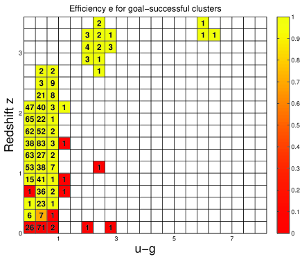
(a) Efficiency in $z$ vs $u-g$ plane (”goal-successful”)

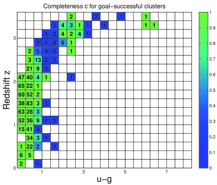
(b) Completeness in $z$ vs $u-g$ plane (”goal-successful”)

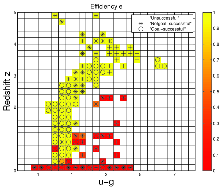
(c) Efficiency in $z$ vs $u-g$ plane (all clusters)

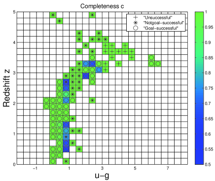
(d) Completeness in $z$ vs $u-g$ plane (all clusters)

Figure 12: Efficiency (upper left-hand panel) and completeness (upper right-hand panel) in the redshift vs ($u-g$) plane for the labelling phase of the first experiment. Colour of the cell is associated to the efficiency and completeness of the selection process of the ”goal-successful” clusters, while the numbers contained in each cell represent the total number of candidates in that region of the $z$ vs $u-g$ plane. Lower left-hand and right hand panels contain the maximum efficiency and completeness for the selection process of the three types of clusters produced by the algorithm. The class of clusters contributing the maximum fraction to the efficiency and completeness represented by the symbol contained in each cell of the plane.

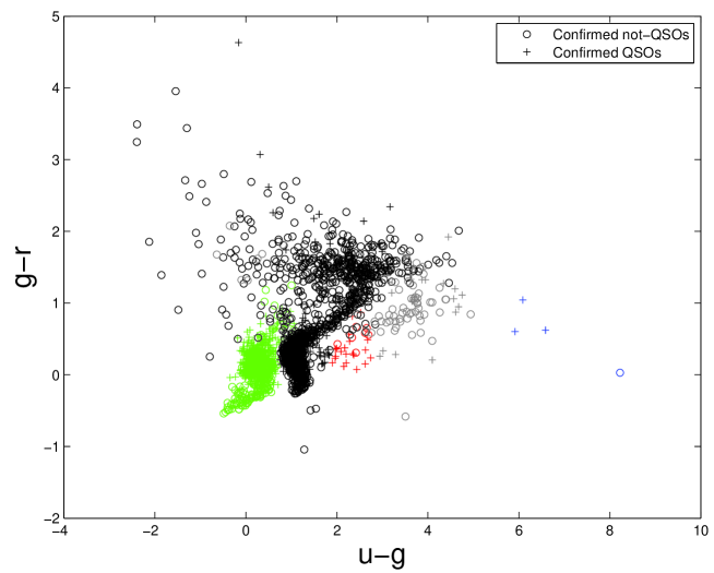
Figure 13: Distribution of S-A sample points in the ($u-g$) vs ($g-r$) plane after the labelling phase of the first experiment. Black and grey symbols are associated respectively to members of the ”notgoal-successful” and ”unsuccessful” clusters, while each single ”goal-successful” cluster is drawn using a different colour. All confirmed QSOs and not QSOs, regardless of their membership, are represented by crosses and circles respectively. Three final ”goal-successful” clusters, green, red and blue respectively, are selected.

5.2 Second experiment

The goal of the second experiment was the selection of candidate quasars inside the optical colour space, using a sample of star-like objects selected in both optical and near infrared catalogues. The number of latent variables used for PPS pre-clustering was again fixed to 62 in order to ease the comparison with the first experiment. The labelling process has been repeated as described in the previous section; the fraction of ”goal-successful” clusters and other parameters of the clustering are shown in the upper left panel of figure (14) as functions of the dissimilarity threshold. The estimated total efficiency and completeness are also plotted as functions of the dissimilarity threshold in the upper right panel of figure (14). The distribution of sources as a function of redshift and spectroscopic classification ”specClass” in the ”goal-successful” clusters selected in this experiment is shown in the middle panel of figure (14) and the ”box and whisker” plot of the distribution of candidate quasars for each of ”goal-successful” clusters is given in the bottom panel of figure (14). The results of this experiment show that our method can reach a significantly higher efficiency and completeness level respect to the optical-infrared candidate selection algorithms found in the literature [Richards et al. 2002, Richards et al. 2004, Warren et al. 1991], using a base of knowledge formed by both ”specClass” for SDSS sources with spectroscopic classification but not selected as quasars candidates and spectroscopic classification of quasars external to SDSS.

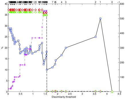
(a) NEC diagnostics

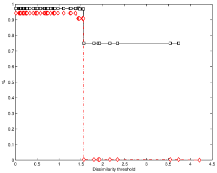
(b) Efficiency and completeness

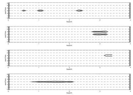
(c) specClass vs redshift plane distribution of clusters

(d) ”Box and wisker” plot of clusters

Figure 14: Same as in the previous figure for the second experiment.

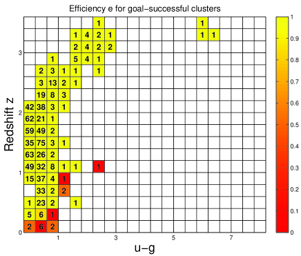
(a) Efficiency in $z$ vs $u-g$ plane (”goal-successful”)

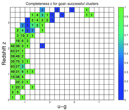
(b) Completeness in $z$ vs $u-g$ plane (”goal-successful”)

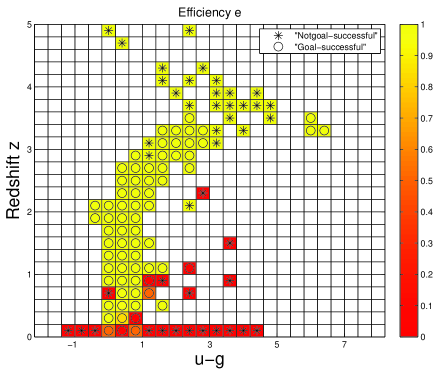
(c) Efficiency in $z$ vs $u-g$ plane (all clusters)

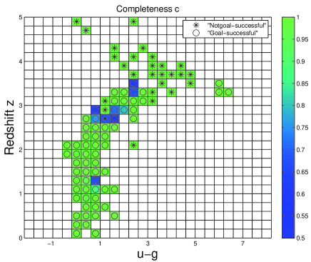
(d) Completeness in $z$ vs $u-g$ plane (all clusters)

Figure 15: Efficiency (upper left-hand panel) and completeness (upper right-hand panel) in the redshift vs ($u-g$) plane for the labelling phase of the second experiment based on the S-UK data set. Colour of the cell is associated to the efficiency and completeness of the selection process of the ”goal-successful” clusters, while the numbers contained in each cell represent the total number of candidates in that region of the $z$ vs $u-g$ plane. Lower left-hand and right hand panels contain the maximum efficiency and completeness for the selection process of the three types of clusters produced by the algorithm. The class of clusters contributing the maximum fraction to the efficiency and completeness represented by the symbol contained in each cell of the plane.

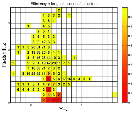
(a) Efficiency in $z$ vs $Y-J$ plane (”goal-successful”)

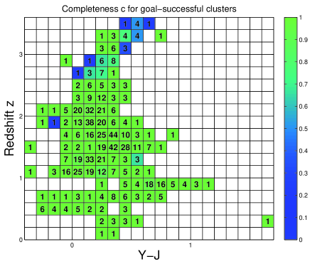
(b) Completeness in $z$ vs $Y-J$ plane (”goal-successful”)

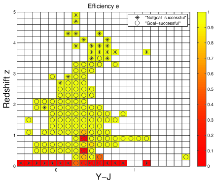
(c) Efficiency in $z$ vs $Y-J$ plane (all clusters)

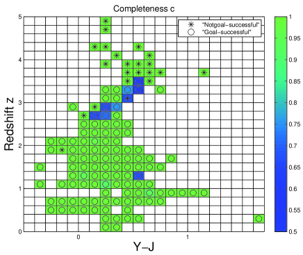
(d) Completeness in $z$ vs $Y-J$ plane (all clusters)

Figure 16: Efficiency (upper left-hand panel) and completeness (upper right-hand panel) in the redshift vs ($Y-J$) plane for the labelling phase of the second experiment based on the S-UK data set. Colour of the cell is associated to the efficiency and completeness of the selection process of the ”goal-successful” clusters, while the numbers contained in each cell represent the total number of candidates in that region of the $z$ vs $Y-J$ plane. Lower left-hand and right hand panels contain the maximum efficiency and completeness for the selection process of the three types of clusters produced by the algorithm. The class of clusters contributing the maximum fraction to the efficiency and completeness represented by the symbol contained in each cell of the plane.

For what the ”goal-successful” clusters are concerned, we can notice that:

• The first cluster is composed of sources with optical $u-g$ colour concentrated around 1.0, while the other optical colours $g-r$, $r-i$ and $i-z$ have average values falling from around 0.7 to 0.5 respectively. The infrared colour $Y-J$ averages at about 0.5, while $J-H$ and $H-K$ increase to mean values of about 0.8 and 1.0. The redshift distribution of this cluster members, all ranked as normal QSOs according to the SDSS spectroscopic classification (”specClass” = 3), shows three different groups of objects situated approximately at $z\sim 0.5,1.1$ and 2.2.

• The second cluster is characterized by a colour distribution similar to the one of the first cluster, except for the optical $u-g$ colour whose mean value increases to 2.0. This cluster is composed of equal fractions of normal and far QSOs according to the ”specClass” index, with a distribution spanning about 0.5 in redshift around 3.

• The third cluster is formed by far QSOs only, with a higher redshift ($z\sim 3.3$) mean value and a colour distribution similar to the second cluster except for a much higher value of $u-g$, with well defined mean at approximately 6.1.

• The last cluster is composed mainly by ”specClass” = 2 sources inside a large redshift interval spanning from $\sim 0.7$ to 2.2. All colours have mean values included between 0.0 and 0.5.

The clusters from second to fourth appear to be very similar to the ”goal-successful” clusters selected in the first experiment both in terms of colours and redshift distribution and spectroscopic type composition. As for the first experiment, the distribution of objects associated to ”goal-successful” clusters during this experiment in two interesting colour-colour planes, namely the mixed optical-infrared colours plane ($r-J$) vs ($J-K$) and the purely optical ($u-g$) vs ($g-r$) plane, is shown in the left-hand and right-hand panel of figure (17) respectively. In the figures (15) and (16) the local values of efficiency and completeness are shown in the redshift vs ($u-g$) and redshift vs ($Y-J$) planes, respectively, with meaning and features of the single plots already explained in the previous paragraph.

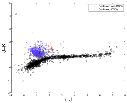
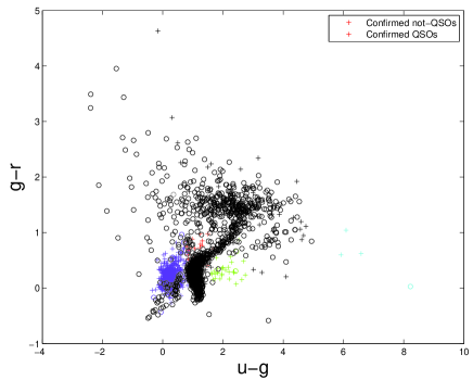
Figure 17: Distribution of S-UK sample points in the ($r-J$) vs ($J-K$) plane (left-hand panel) and ($u-g$) vs ($g-r$) plane (right-hand panel) after the labelling phase of the second experiment. Black and grey symbols are associated respectively to members of the ”notgoal-successful” and ”unsuccessful” clusters, while each single ”goal-successful” cluster is drawn using a different colour. All confirmed QSOs and not QSOs, regardless of their membership, are represented by crosses and circles respectively.

5.3 Third experiment

The third experiment was carried out in order to test whether the addition of the near infrared colours to the optical colours already used as parameters for the first two experiments improves or not the total efficiency and completeness of candidate quasars selection. In conformity to the previous experiments, the number of latent variables was fixed to 62, resulting in an equal number of pre-clusters produced. As in the previous experiments, all relevant information are reported in figure (18).

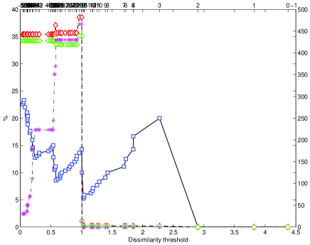
(a) NEC diagnostics

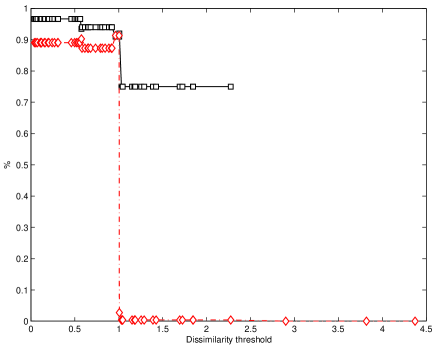
(b) Efficiency and completeness

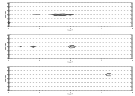
(c) specClass vs redshift plane distribution of clusters

(d) ”Box and wisker” plot of clusters

Figure 18: Same as in the previous figure for the third experiment.

Table 4: Description of the contents of ”goal-successful” clusters selected in the experiments carried out. For each cluster, the total number of members $n$ and the fraction of confirmed quasars are reported.

Exp.	Cluster	% quasars	$n$
1	1	75.9%	29
	2	81.5%	957
	3	75.1 %	4
2	1	76.1%	652
	2	83.3%	48
	3	100.0%	4
3	1	92.3%	26
	2	93.5%	31
	3	75.0%	4
	4	97.7%	755
4	1	86.2%	2121
	2	93.1%	52190
	3	77.9%	2433
	4	75.8%	198
	5	78.6%	126
	6	90.6%	171
	7	91.5.%	298
	8	78.9%	90
	9	79.0%	76
	10	86.1%	92

The results of this experiment are summarised in the following description of the ”goal-successful” clusters selected.

• The mean values of colours distribution of the members of the first cluster range from 0.0 to 0.5 with outliers mainly situated at higher values, while the distribution of normal QSOs in redshift spans from 0.7 to 2.2 and a little contamination from ”specClass = 1” stars is present.

• The second cluster, entirely composed by ”specClass” = 2 sources, shows a colours distribution almost identical to the previous cluster, while the distribution in redshift peaks at $z\sim 0.4,0.7$ and 2.1.

• The third clusters contains sources with a value of $u-g\sim 6$ and $g-r\sim 1$, while the other two colours have distributions consistent with zero. This cluster is formed by far QSOs with redshift higher than 3.0.

(a) Efficiency in $z$ vs $u-g$ plane (”goal-successful”)

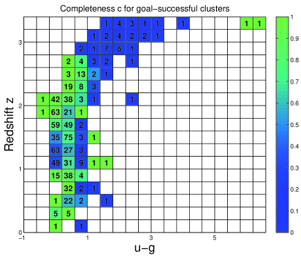
(b) Completeness in $z$ vs $u-g$ plane (”goal-successful”)

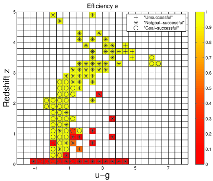
(c) Efficiency in $z$ vs $u-g$ plane (all clusters)

(d) Completeness in $z$ vs $u-g$ plane (all clusters)

Figure 19: Efficiency (upper left-hand panel) and completeness (upper right-hand panel) in the redshift vs ($u-g$) plane for the labelling phase of the third experiment based on the S-UK data set though using only optical photometry. Colour of the cell is associated to the efficiency and completeness of the selection process of the ”goal-successful” clusters, while the numbers contained in each cell represent the total number of candidates in that region of the $z$ vs $u-g$ plane. Lower left-hand and right hand panels contain the maximum efficiency and completeness for the selection process of the three types of clusters produced by the algorithm. The class of clusters contributing the maximum fraction to the efficiency and completeness represented by the symbol contained in each cell of the plane.

Also in this case, the clusters selected are very similar in terms of colours and redshift distributions to the ”goal-successful” clusters selected in the previous, two experiments. The distribution of ”goal-successful” candidates in the optical colour-colour ($u-g$) vs ($g-r$) plane is shown in figure (20). The figure (19) contains the local values of the efficiency and completeness in the redshift vs ($u-g$) plane for the third experiment for the ”goal-successful” only and all the three kind of clusters determined by the labelling in the upper and lower panels, respectively.

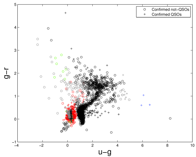
Figure 20: Distribution of S-UK sample points in the ($u-g$) vs ($g-r$) plane after the labelling phase of the third experiment. Black and grey symbols are associated respectively to members of the ”notgoal-successful” and ”unsuccessful” clusters, while each single ”goal-successful” cluster is drawn using a different colour. All confirmed QSOs and not QSOs, regardless of their membership, are represented by crosses and circles respectively.

5.4 Fourth experiment

The fourth experiment was carried out as an application to the SDSS candidate quasars data set of the algorithm described in this paper. Also in this case the number of latent variables for the PPS algorithm was fixed to 62. Results are shown in figure (21).

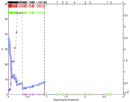
(a) NEC diagnostics

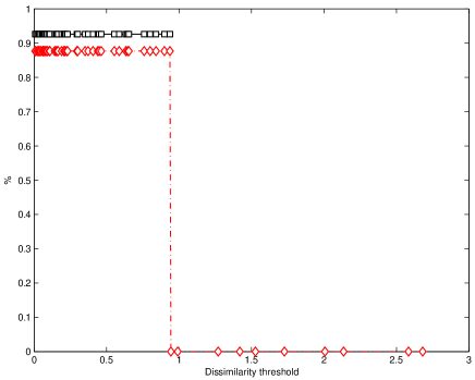
(b) Efficiency and completeness

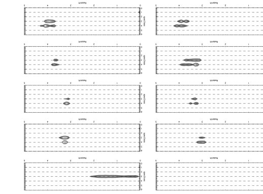
(c) specClass vs redshift plane distribution of clusters

(d) ”Box and wisker” plot of clusters

Figure 21: Same as in the previous figure for the fourth experiment.

• The first cluster is composed mainly by normal QSOs situated at low redshift, having $u-g$, $r-i$ and $i-z$ colours with means ranging form 0.0 to 0.5, and the $g-r$ colour with an average value slightly higher and centred on $\sim 1.0$.

• The distributions of colours of the members of the second cluster all peak at about 0.0 with outliers reaching higher values especially in $r-i$ and $i-z$ colours. The distribution in redshift of the sources of this cluster, formed exclusively by ”specClass” = 3 normal QSOs, spans the whole interval from $\sim 0.0$ to 2.2.

• The remaining ”goal-successful” clusters selected in this experiment show as common feature distributions of $u-g$ with higher means than previous clusters, ranging from $\sim 2$ to $\sim 5.5$. The $g-r$ colours are instead distributed between 1.8 and $\sim 0.2$ and the others colours have similar mean values around 0. All these clusters are formed by a mixture of normal and far QSOs according to the SDSS spectroscopic classification, with redshifts going from 3 to 4.2.

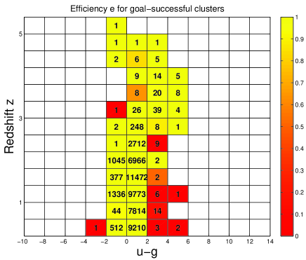
(a) Efficiency in $z$ vs $u-g$ plane (”goal-successful”)

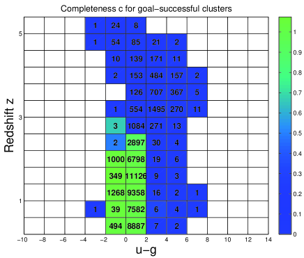
(b) Completeness in $z$ vs $u-g$ plane (”goal-successful”)

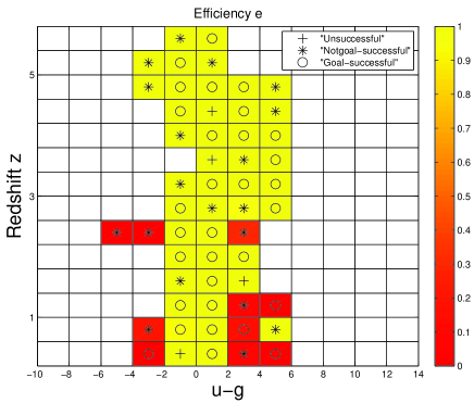
(c) Efficiency in $z$ vs $u-g$ plane (all clusters)

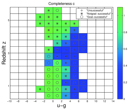
(d) Completeness in $z$ vs $u-g$ plane (all clusters)

Figure 22: Efficiency (upper left-hand panel) and completeness (upper right-hand panel) in the redshift vs ($u-g$) plane for the labelling phase of the fourth experiment based on the S-S data set. Colour of the cell is associated to the efficiency and completeness of the selection process of the ”goal-successful” clusters, while numbers contained in each cell represent the total number of candidates in that region of the $z$ vs $u-g$ plane. Lower left-hand and right hand panels contain the maximum efficiency and completeness for the selection process of the three types of clusters produced by the algorithm. The class of clusters contributing the maximum fraction to the efficiency and completeness represented by the symbol contained in each cell of the plane.

The distribution of ”goal-successful” candidates in the ceentral region of the optical colour-colour ($u-g$) vs ($g-r$) plane for the fourth experiment is shown in figure (23), while the local values of efficiency and completeness for the labelling phase of the same experiment are shown in figure (22).

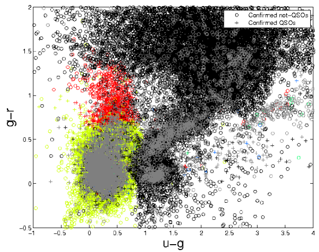
Figure 23: Distribution of S-S sample points in the ($u-g$) vs ($g-r$) plane after the labelling phase of the fourth experiment. Black and grey symbols are associated respectively to members of the ”notgoal-successful” and ”unsuccessful” clusters, while each single ”goal-successful” cluster is drawn using a different colour. All confirmed QSOs and not QSOs, regardless of their membership, are represented by crosses and circles respectively.

5.5 Comparison of the results

The estimates of the efficiency and completeness of the experiments described in the previous paragraphs show that the method successfully recover a very high fraction of the spectroscopic QSOs when the BoK is based on the spectroscopic classification provided by the SDSS. The differences in the performances of the selection process are due to the different criteria used to select the samples of sources used for the training of the method in the different experiments. The results obtained in the four experiments can be summarized as it follows:

• First experiment (optical BoK and parameter space): the S-A sample composed by unresolved objects belonging to the ”Star” table of the SDSS database and placed in the overlapping regions between SDSS-DR1 and UKIDSS-DR1 LAS surveys, together with a BoK represented by the ”specClass” spectroscopic classification index are used. Optical colours are employed as parameters. The highest performance is reached with a total efficiency $e_{tot}=81.5\%$ and a completeness $c_{tot}=89.3\%$, within $n_{gen}=2$ generations of clustering.

• Second experiment (optical + near infrared BoK and optical parameter space): the S-UK sample obtained selecting only the sources observed in both SDSS and UKIDSS-DR1 LAS surveys and classified as stars in both surveys, together with a BoK represented by the SDSS ”specClass” spectroscopic classification index are used. Optical colours are employed as parameters. The best performance is reached with a total efficiency $e_{tot}=92.3\%$ and a completeness $c_{tot}=91.4\%$, within $n_{gen}=1$ generation of clustering. This experiment shows a significant improvement of the total efficiency and a slight improvement of the total completeness over the previous experiment.

• Third experiment (optical + near infrared BoK and parameter space): the same sample and BoK of the previous experiment are used. Optical and near infrared colours are employed as parameters. The best performance is reached with a total efficiency $e_{tot}=97.2\%$ and a completeness $c_{tot}=94.3\%$, within $n_{gen}=1$ generation of clustering. The addition of infrared photometric informations improves both efficiency and completeness of the candidate quasars selection process.

• Fourth experiment (optical BoK and parameter space): the S-S sample composed by all the candidate quasars according to the native SDSS candidate QSOs selection algorithm in the whole DR5 database ”Target” table, and the same BoK of the previous experiments are used. Only optical colours are employed as parameters. The best performance is reached with a total efficiency $e_{tot}=95.4\%$ and a completeness $c_{tot}=94.7\%$, within $n_{gen}=3$ generations of clustering.

The most significant experiments, in terms of selection performances, appear to be the second and third ones, which take into account also part of the so-called ”optically dull” quasars, i. e. those objects which show very little signature in the optical bands and are usually selected as QSOs by means of additional information of spectroscopic nature or, like in this case, of photometric nature (near infrared colours). The increase in efficiency between the first and second experiments, even if the parameter space has not been modified, is due to the fact that the BoK used for the second experiment is formed by sources that have been observed in both optical and near infrared bands and in both bands have been confirmed as QSOs. The different BoK represents a more specific family of QSOs (emitting strongly in NIR) whose location in the colour space is more easily traceable than the whole class of QSOs observed in the optical colours. The only slight increase in efficiency observed in the third experiment with respect to the second, caused by to the addition of near infrared colours to the photometric parameter (which allows to resolve more efficiently part of the degeneracies in the colour distribution between stars and QSOs), confirms that this method is much more sensitive to the features of the BoK that to the number of dimensions of the parameter space where the unsupervised clustering is carried out. The fourth experiment shows that this method can be applied to a large BoK composed by stellar sources which have received spectroscopic observation to perform the selection of photometric candidate QSOs. The same kind of experiment, even if with a different BoK, has been performed to extract the original catalogue of QSOs candidates described in section (7).

6 The selection of the parameters

In this section we shortly discuss how the performances of our candidate quasars selection method depend upon the assumed parameters of the PPS and NEC algorithms respectively, and on the set of features used for the characterization of the distribution of objects inside the parameter space. More specifically, we have focused our attention on the dependance of the performance of the PPS algorithm on the number of latent variables (i.e. the number of preclusters produced by PPS), the dependance of the NEC algorithm on the critical value of the dissimilarity threshold $T_{cr}$, and the dependance of the overall method from the particular set of colours used to define the parameter space inside which the clustering is performed.

6.1 Dependence on PPS parameter

As it has been discussed elsewhere, the PPS performances are rather independent on the choice of the parameters (clamping factor, width and orientation of principal surfaces, tolerance and number of iterations), with the exception of the number of latent variables. This number needs to be neither too large nor too small (within rather large boundaries) An excessive number of latent variables produces clusters that are not agglomerated efficiently by the NEC algorithm, while setting the number of latent variable to a low number does not allow a proper separation of different groups of objects in distinct clusters. In absence of theoretical ways to estimate the correct number of latent variables, the only way is to guess it through a trial and error procedure. It needs to be stressed that even though rather demanding in terms of computing time, for a given problem and data set, this procedure needs to be run only once.

6.2 Dependence on colours choice

In order to detect any bias introduced by the choice of a particular colours set in the results, all experiments have been repeated using colours derived by different combination of magnitudes (table (5)) and keeping unchanged all the other parameters. These tests showed that the total efficiency $e_{tot}$ and completeness $c_{tot}$ are robust with respect to the particular parameter space where the distribution of objects is studied. Fluctuations affecting both $e_{tot}$ and $c_{tot}$ for all possible sets of parameters are, in the worst cases, comparable with few percents of the optimal values obtained using the natural combination of colours. This result can be understood from a theoretical point of view remembering that, given an initial set of colours $C_{0}$ derived from a certain photometric system, all other possible colours sets $C_{i}$ can be expressed as linear combinations of $C_{0}$, so that each parameter space $\Sigma_{i}$ generated by $C_{i}$ is the result of the application of a rigid rotation to the the parameter space $\Sigma_{0}$ associated to $C_{0}$. The transformation applied to the parameter space does not affect the relative positions and distances between points of the distribution and, as a consequence, the principal curves or surfaces generated by PPS algorithm in order to determine the best projection from the generic parameter space $\Sigma_{i}$ to the latent space remain unchanged.

Experiment	Colours	$e_{tot}$	$c_{tot}$
1	natural	81.5%	89.3%
1	($u-r$, $g-i$, $r-z$, $i-u$)	81.7%	89.5%
1	($u-i$, $g-z$, $r-g$, $i-r$)	80.8%	89.3%
1	($u-z$, $g-u$, $r-z$, $i-r$)	82.0%	89.0%
1	($u-g$, $g-z$, $r-i$, $i-z$)	81.4%	89.7%
2	natural	92.3%	91.4%
2	($u-r$, $g-i$, $r-z$, $i-u$, $Y-H$, $J-K$, $H-Y$)	92.3%	91.5%
2	($u-i$, $g-z$, $r-g$, $i-r$, $Y-K$, $J-Y$, $H-J$)	92.7%	91.8%
2	($u-z$, $g-u$, $r-z$, $i-r$, $Y-H$, $J-K$, $H-Y$)	91.9%	90.9%
2	($u-Y$, $g-H$, $r-J$, $i-K$, $z-u$, $Y-g$, $H-r$)	91.0%	91.0%
2	($u-H$, $g-J$, $r-K$, $i-u$, $z-g$, $Y-z$, $H-i$)	90.9%	91.2%
2	($u-J$, $g-K$, $r-u$, $i-g$, $z-r$, $Y-i$, $H-z$)	92.2%	91.5%
2	($u-z$, $g-K$, $H-J$, $z-Y$, $r-u$, $z-i$, $i-H$)	92.6%	91.4%
3	natural	97.3%	94.3 %
3	($u-r$, $g-i$, $r-z$, $i-u$)	97.1%	94.8 %
3	($u-i$, $g-z$, $r-g$, $i-r$)	97.0%	93.9 %
3	($u-z$, $g-u$, $r-g$, $i-r$)	97.3%	94.0 %
3	($u-g$, $g-z$, $r-i$, $i-z$)	96.9%	94.9%
4	natural	94.5%	93.0%
4	($u-r$, $g-i$, $r-z$, $i-u$)	95.2%	93.9%
4	($u-i$, $g-z$, $r-g$, $i-r$)	95.0%	94.0%
4	($u-z$, $g-u$, $r-g$, $i-r$)	95.4%	94.4%
4	($u-g$, $g-z$, $r-i$, $i-z$)	95.7%	94.6%

Table 5: Efficiency and completeness for the three experiments evaluated using sets of different colours. The natural combinations of colours corresponds, by definition, to ($u-g$, $g-r$, $r-i$, $i-z$) for the experiments making use of only optical colours, and ($u-g$, $g-r$, $r-i$, $i-z$, $Y-J$, $J-H$, $H-K$) for the experiment making use of both optical and infrared colours. Only a selection of all permutations is shown.

6.3 Dependence on clustering algorithm parameter

The choice of the thresholds $\widetilde{sr}^{(g)}$ and $\widetilde{sr}^{(ng)}$ introduced in the definitions of ”goal-succcessful” and ”notgoal-successful” clusters, respectively, only affects the total time required by algorithm in order to converge, i. e. the number of generations needed to select all possible candidate quasars in a given sample. The only requirement is that these thresholds need to be included in an interval of reasonable values (in this case, we have tested values of this parameter in the range [0.65, 0.90]). Lower values of the thresholds would allow the algorithm to select many clusters with a very high level of contamination from ”notgoal” objects (”goal” objects) at the cost of a reduction of the overall efficiency, while higher values would make practically impossible the selection of a major fraction of candidates, since only few clusters composed almost by only ”goal” (”notgoal”) sources would conform to the definition.

6.4 Local estimates of efficiency and completeness

The overall trends in the local estimates of the efficiency $e$ and completeness $c$ in the redshift vs colour planes for the various experiments described in the above paragraphs, carry useful information on the performances of the algorithm and on the utility of the BoK. Even if the samples used for the experiments are slightly different, the main features of the efficiency and completeness plots can be traced back to the same properties of the general distribution of QSOs in the photometric parameter space.

1. In almost all plots showing the local values of efficiency calculated for the experiments examined in the present paper (for example, see upper-left panels of figures (12), (15) and (19)), few cells with lower values of $e$ are found for low values of the redshift. This effect does not seem to depend on the specific colour since a similar systematic is visible, for example, in the upper-left panels of figures (15) and (16), where $e$ has been evaluated in both the z vs $(u-g)$ and z vs $(Y-J)$ planes respectively for the second experiment. Another interesting feature of these local estimates of the efficiency is the presence of two distinct clumps of cells populated by few members of the BoK located at high redshift and approximately around $(u-g)\approx 2.2$ and $(u-g)\approx 6.2$. These clumps can be immediately associated to two ”goal-successful” clusters visible in the $u-g$ vs $g-r$ plot (see figure (13)) around similar values of the $u-g$ colour. These two features of the local estimates of the efficiency, while clearly visible in the case of the first experiment (left-hand panel of figure (12)), do not show up in the same plots for the second and third experiments (left-hand panels of figures (15) and (19)) where only the first and the second clump can be seen, respectively.

2. In almost all plots showing the local values of the completeness in the z vs $(u-g)$ plane (see the upper right-hand panels of figures (12), (15) and (19)), a region with low values of $c$ is found for redshifts in the range $[2.4,3.2]$ and $(u-g)$ colour from $\approx 1$ to $\approx 3$ for the first three experiments. These regions are more or less extended according to the experiment considered and to the widths of the bins used to determine the tessellation of the z vs $(u-g)$ plane. In terms of total completeness for each experiment, the number of confirmed QSOs lost in these underpopulated regions of the parameter space in nonetheless low, namely $\approx 5\%$ of the total number of confirmed QSOs in the BOK for the first experiment, and $\approx 3\%$ and $\approx 7\%$ for the second and third experiments respectively.

3. All the efficiency and completeness plots show a lack of members of the BoK can be noticed in the upper left corners of the plots, roughly corresponding to a triangular region going from z $\approx 2$ to the upper limit of the redshift distribution, and on the other axis spanning approximately the interval $[-0.5,1]$ for the $u-g$ colour and the interval $[-0.4,0.4]$ along the $Y-J$ colour axis. This selection effect depends on the nature of the BoK (i.e. on the selection criteria for the spectroscopic targets of the SDSS survey) used to perform the experiments (cf. [Stoughton et al. 2002, Richards et al. 2002]) and is not caused in any regard by the selection method here discussed.

4. The plots showing which type of clusters contributes most to the efficiency and completeness inside each cell of the redshift vs colour plane (lower panels of figures (12), (15) and (19)) indicates that ”goal-successful” clusters dominate the regions where the efficiency and completeness of the QSOs candidate selection are almost unitary, as can be seen comparing these plots with the local efficiency plots and completeness (for examples, in the first experiment, compare the upper-left and lower-left side panels for the efficiency and the upper-right and lower-right panels for the completeness of figure (12)). ”Notgoal-successful” clusters, on the other hand, are mainly found in places of the redshift vs colour plane corresponding to the regions of the parameter space occupied by the ”stellar locus” which can be easily singled out in the colour-colour plots (figure (13), left-hand panel in figure (17) and figure (20)). ”Unsuccessful” clusters, i.e. clusters composed of similar fractions of confirmed QSOs and contaminant, in the first and third experiments, are usually dominant in the neighbourhood of the almost isolated and underpopulated regions of the plane where groups of few cells with unitary efficiency are located (high redshift and high value of the $(u-g)$ colour, see above for details). In these experiments few other cells in both efficiency and completeness plots are dominated by the contribution from unsuccessful clusters, while no cell of this type is determined for the second experiment.

It should be emphasised that all the systematic effects and biases here discussed and affecting the selection of the QSOs, though not hindering this candidate selection method from achieving performances significantly better than those produced by more classical algorithms found in the literature, are merely reflections and consequences of the same systematics and biases affecting the spectroscopic data set used to constitute the base of knowledge for the labelling phase of our method. We can therefore conclude that the improvement of this method is subordinate to the enhancement of the coverage of the photometric parameter space sampled by the spectroscopic data and to the improvement of the accuracy of the estimates of both spectroscopic and photometric observables making up the parameter space and the labels to be used during the unsupervised clustering phase of the algorithm.

7 The catalogue of candidate QSOs

The application of our algorithm to a base of knowledge composed of all stellar sources with spectroscopic observations (see (7.1) for details) extracted from the SDSS DR7 Legacy has produced the clustering in the photometric parameter space used to select the QSOs candidates from a suitable catalogue of sources extracted from the SDSS DR7 photometric dataset. The next sections describe in detail the nature of the spectroscopic BoK used to determine the partition of the parameter space and of the photometric samples of objects from which the candidate QSOs have been extracted (7.1), the process of the extraction of the catalogue and its characterization (7.3), the expected completeness and efficiency of the catalogue (7.2), the comparison with one the catalogues of photometric QSO candidates available in the literature (7.4) and a first astronomical application of the catalogue of candidates, namely the number counts derived from our candidate QSOs (7.5).

7.1 The base of knowledge

The dataset (hereafter S-SCat) used as BoK for the extraction of the QSO candidates from the SDSS photometric database is composed by all the primary (”mode” = 1) stellar sources belonging to the PhotoObjAll table of the DR7 data release (i.e. identified as point-like sources according to a purely photometric criterion, i.e. $"type"=6$) with standard clean photometry (for all dereddened psf magnitudes) in all SDSS bands, reliable spectroscopic classification (with ”specClass” = 1, 3, 4, 6, 0) and reliable spectroscopic redshift estimate (”zConf”$>0.95$). In order to avoid the inclusion in S-SCat of faint or saturated sources, following [Richards et al. 2008], a further constraint on the $i$ magnitude has been applied, requiring that $psfMag_{i}>14.5$ and $(psfMag_{i}-extinction_{i})<21.3$. The S-SCat dataset, regardless of the status of each member as QSO candidates according to the native SDSS candidate selection algorithm, has been used to reconstruct the distribution of spectroscopically confirmed QSOs and stars inside the SDSS colours space by the identification of ”goal-successful” and ”notgoal-successful” clusters using the unsupervised clustering method discussed in this paper. The total number of sources belonging to the S-SCat dataset and the fractions of different type of sources according to the spectral classification expressed by the ”specClass” index are shown in table (1). The distribution of the spectroscopic redshift of the S-SCat and the distribution in magnitude are shown in figures (24) and (25) respectively.

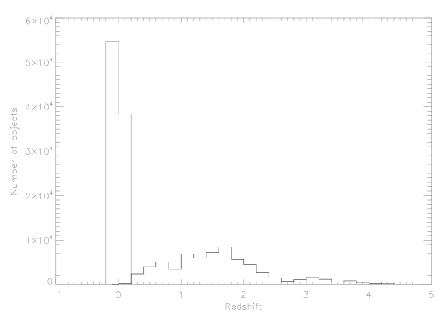
Figure 24: Redshift distribution of the S-SCat sample. The grey line represents the distribution of stars and unknown sources according to the ”specClass” (”specClass” $=\{1,6,0\}$) classification while the black line is associated to QSOs (”specClass” $=\{3,4\}$).

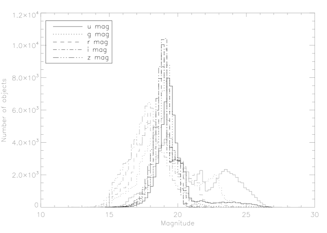
Figure 25: Distribution in luminosity of the sources belonging to the S-SCat sample. The grey lines represent the distribution of stars and unknown sources according to the ”specClass” classification (”specClass” $=\{1,6,0\}$), while the black lines are associated to QSOs (”specClass” $=\{3,4\}$).

7.2 S-SCat experiment: efficiency and completeness

Table 6: Main features of the ”goal-successful” clusters determined during the S-SCat experiment with the position of the centres of mass (”CoM”) of the clusters in the colours space.

Cluster Index	1	2	3	4	5	6	7	8	9	10
Nm elements	1326	54368	3429	835	741	273	622	486	2491	595
Nm confirmed	1135	50012	3250	592	636	206	546	380	2057	550
Nm not-confirmed	191	4345	179	242	105	67	75	106	434	45
confirmed/total	0.86	0.92	0.95	0.71	0.86	0.75	0.88	0.78	0.83	0.92
not-confirmed/total	0.14	0.08	0.05	0.29	0.14	0.25	0.12	0.22	0.17	0.08
CoM $u-g$ position	0.40	0.21	0.53	4.33	2.32	0.63	0.52	5.34	0.53	1.98
CoM $g-r$ position	0.42	0.12	0.04	0.82	0.34	0.06	0.46	0.90	0.40	0.23
CoM $r-i$ position	0.41	0.12	0.03	0.17	0.10	-0.15	0.15	0.20	0.13	0.08
CoM $i-z$ position	0.17	0.04	0.24	0.11	0.06	0.31	0.50	0.13	0.14	0.06

The number of latent variables (i.e. pre-clusters) produced by the PPS in the S-SCat experiment is 146 and the critical value of the dissimilarity threshold has been chosen according to the criteria explained in the previous paragraphs. The best clustering is produced for a value of the dissimilarity threshold $D_{th}=0.20$ corresponding to a final number of ”goal-successful” clusters equal to 10, whose main characteristics are summarized in the table (6). The normalised success ratio and other statistical indicators of the clustering process as functions of the dissimilarity threshold $D_{th}$ are shown in figure (26), while the estimated efficiency and completeness of the selection process are shown in figure (27) as functions of the dissimilarity threshold as well. The distribution of sources as a function of redshift and spectroscopic classification ”specClass” in the ”goal-successful” clusters produced in this experiment is shown in figure (28), while the main features of the distribution of sources associated to the ”goal-successful” clusters of experiment S-SCat in the parameter space can be summerized and described through the ”box and whisker” plots (see figure (29)).

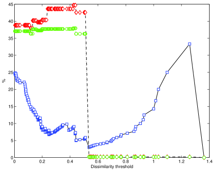
Figure 26: The fraction of ’goal-successful’ clusters (squares), the total percentage of the sources of the BoK belonging to ’goal-successful’ clusters (circles), the total percentage of objects belonging to ’goal-successful’ clusters irrespective of their spectroscopic classification (diamonds) are plotted as a function of the dissimilarity threshold for the S-SCat experiment.

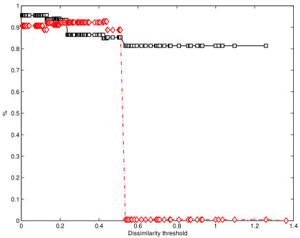
Figure 27: Total estimated efficiency $e_{tot}$ (squares) and completeness $c_{tot}$ (diamonds) of the candidate QSOs selection process as functions of the dissimilarity threshold are plotted for the S-SCat experiment.

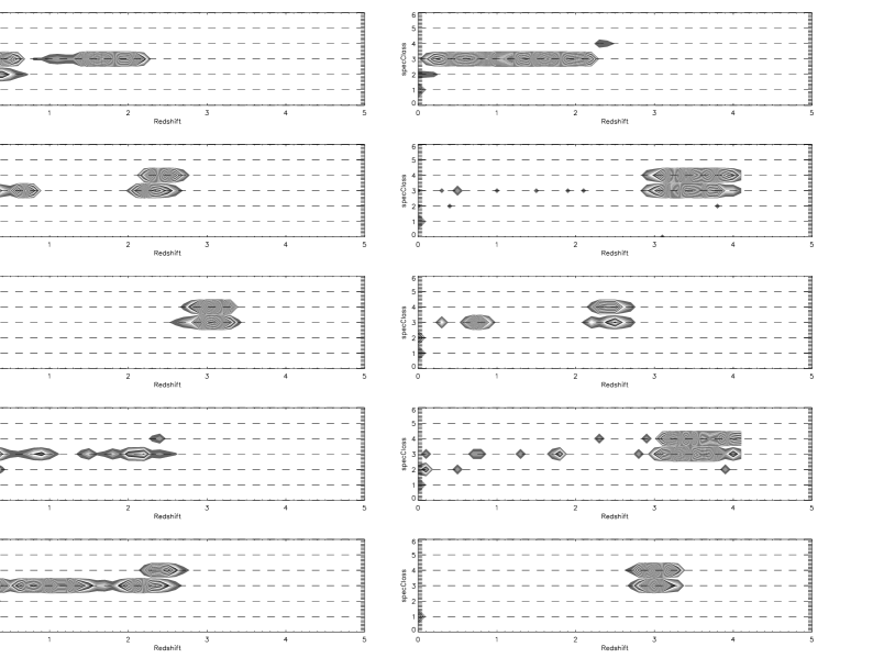
Figure 28: Distribution of members of the 10 ”goal-successful” clusters determined during the S-SCat experiment in the ”specClass”-redshift plane (cluster 1 to cluster 10 from left to right and from top to down).

Figure 29: ”Box and whisker” plots of the distribution of clusters produced in the experiment S-SCat (cluster 1 to cluster 10 from left to right and from top to down).

In what follows, a brief description of the characteristics of the distributions of sources associated to the 10 ”goal-successful” clusters selected in the S-SCat experiment, in terms of colours, redshift and classification is given:

• Cluster 1: formed by sources having $u-g$, $g-r$ and $r-i$ colours centered at about 0.4 and $i-z$ with slightly smaller average ($\sim 0.2$). The members of this cluster are mainly QSOs and galaxies, according to the ”specClass” classification, spanning in redshift from from 0 to 2.3. No ”specClass” = 4 quasars (according to the SDSS classification) are found. A small fraction of contaminant galaxies (”specClass” = 2) is present at $z_{spec}<0.6$

• Cluster 2: composed by a very large fraction of ”specClass” = 3 QSOs and few galaxies and ”specClass” = 4 quasars, all located in the $[0,2.5]$ redshift interval. The colours distribution of the members of this cluster is characterized by very similar average for all four colours, approximately located at 0.2.

• Cluster 3: this cluster shows a widespread $u-g$ distribution centered around 0.5, with $g-r$ and $r-i$ colours distributions peaked around 0 and $i-z$ with average $\sim 0.2$. The members of this cluster are almost totally ”specClass” = 3 and ”specClass” = 4 QSOs located in two different regions in redshift, namely the intervals $[0,1]$ and $[2,2.8]$ respectively. Very few ”specClass” = 1 stars can be found.

• Clusters 4 and 5: both these clusters are mostly populated by QSOs classified as ”specClass” = 3 and 4 according to the SDSS spectroscopic classification. The redshift distributions are different: both clusters have their lowest edge approximately at the $z_{spec}\sim 2.5$ but cluster 5 reaches redshifts slightly higher than 4 while cluster 4 is contained in the $[2.5,3.3]$ interval. The colour distributions are similar, with $g-r$, $r-i$ and $i-z$ colours peaked between 0 and 0.6, while the $u-g$ colour has a remarkably high average in the fourth cluster (at $\sim 4$) while reaching $\sim 2.3$ for the cluster 5.

• Cluster 6: this cluster shows $u-g$, $g-r$, $r-i$ and $i-z$ colours centered around 0.6, 0.0, -0.1 and 0.3 respectively, with a large dispersion for $g-r$ and $r-i$. It is mainly formed by ”specClass” = 3 and 4 QSOs, with redshift distribution very similar to that of cluster 3. Few stars (”specClass” = 1) and galaxies (”specClass” = 2) can be found.

• Cluster 7: mainly formed by ”specClass” = 3 QSOs spanning the redshift range from $\sim 0.1$ to 0.5, few ”specClass” = 4 quasars and galaxies are also present, located at $z_{spec}\sim 0.3$ and $z_{spec}\sim 2.2$ respectively. Colours distributions are centered between 0 and 0.5 with large dispersions around the averages.

• Cluster 8: the colours distribution is very similar to the distribution of cluster 4, with $u-g$ reaching even larger average ($\sim 5.2$ instead of $\sim 4$.) Composition and redshift distribution are also similar to those of cluster 4, with a slightly higher fraction of contaminants represented by galaxies (”specClass” = 2) and stars (”specClass” = 1).

• Cluster 9: formed mainly by ”specClass” = 3 and 4 QSOs with redshift to 2.6, there is a significant fraction of galaxies in the $z_{spec}$ interval from $\sim 0$ to 0.3. Colours distributions are peaked around 0.5, 0.4, and 0.2 for $u-g$ , $g-r$ and the remaining two colours respectively.

• Cluster 10: very similar to the cluster 4 and 5 in terms of colours distribution, it is almost exclusively composed by ”specClass” = 3 and 4, with redshifts around 3 in the interval $[2.7,3.3]$.

The local values of the efficiency and completeness of the selection process in the redshift vs colour and colour vs colour planes for the ”goal-successful” clusters, evaluated using the BoK of the S-SCat experiment, are shown in figures (30, 31) and (32, 33) respectively. The meaning of these plots is described in section (5). These plots can be used to inspect on a local scale the efficiency and completeness of the selection process in termes of colours and redshifts of the members of the BoK used for the experiment S-SCat. A more general view of the partition of the parameter space produced during the S-SCat experiment can be seen in figures (34) and (35), where the local efficiency and completeness of the selection process are shown in the colour vs colour planes for all types of clusters (i. e., not only ”goal-successful”, but also ”notgoal-successful” and”unsuccessful” clusters). The meaning of the symbols is also explained in section (5).

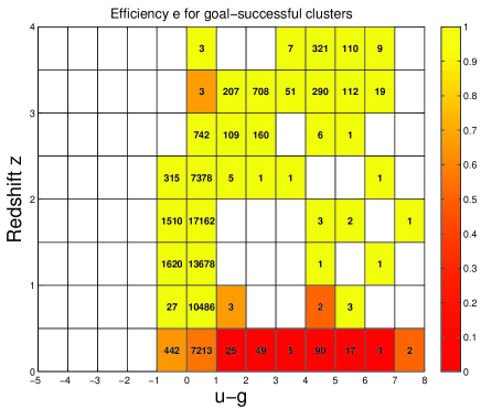
(a) Efficiency in $z$ vs $u-g$ plane

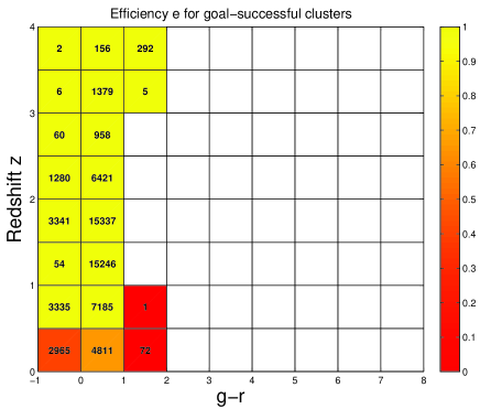
(b) Efficiency in $z$ vs $g-r$ plane

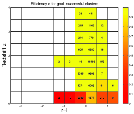
(c) Efficiency in $z$ vs $r-i$ plane

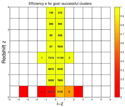
(d) Efficiency in $z$ vs $i-z$ plane

Figure 30: Local efficiency estimates in the redshift vs colour planes for the ”goal-successful” clusters of experiment S-SCat. Numbers represent the total number of sources of the BoK located in each cell.

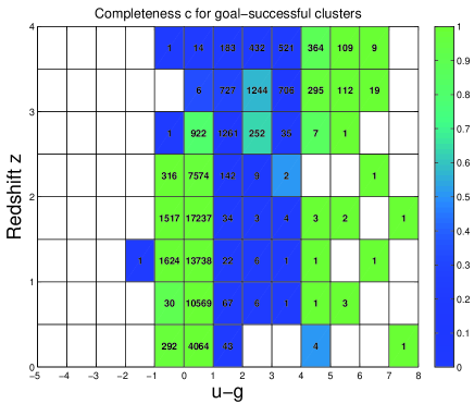
(a) Completeness in $z$ vs $u-g$ plane

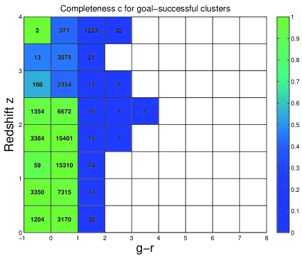
(b) Completeness in $z$ vs $g-r$ plane

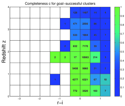
(c) Completeness in $z$ vs $r-i$ plane

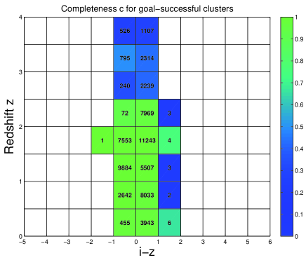
(d) Completeness in $z$ vs $u-g$ plane

Figure 31: Local completeness estimates in the redshift vs colour planes for the ”goal-successful” clusters of experiment S-SCat. Numbers represent the total number of sources of the BoK located in each cell.

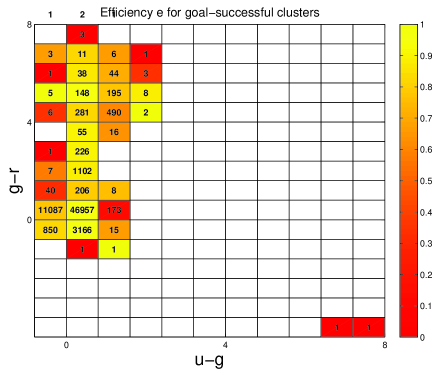
(a) Efficiency in $u-g$ vs $g-r$ plane

(b) Efficiency in $u-g$ vs $r-i$ plane

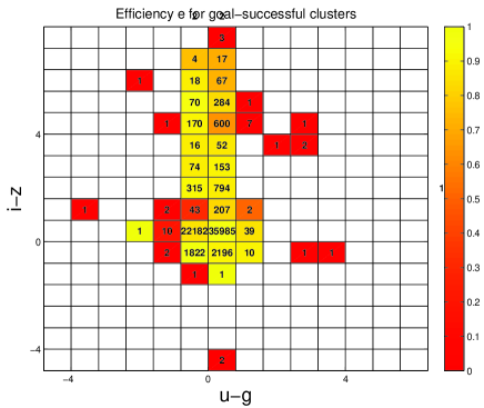
(c) Efficiency in $u-g$ vs $i-z$ plane

(d) Efficiency in $g-r$ vs $r-i$ plane

(e) Efficiency in $g-r$ vs $i-z$ plane

(f) Efficiency in $r-i$ vs $i-z$ plane

Figure 32: Local efficiency estimates in the colour vs colour planes for the ”goal-successful” clusters of experiment S-SCat. Numbers represent the total number of sources of the BoK located in each cell.

(a) Completeness in $u-g$ vs $g-r$ plane

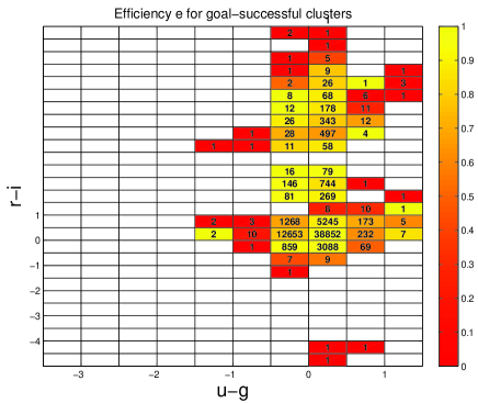
(b) Completeness in $u-g$ vs $r-i$ plane

(c) Completeness in $u-g$ vs $i-z$ plane

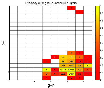
(d) Completeness in $g-r$ vs $r-i$ plane

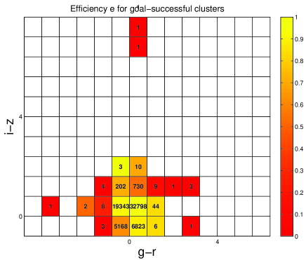
(e) Completeness in $g-r$ vs $i-z$ plane

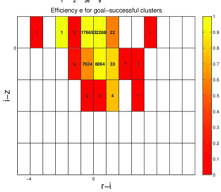
(f) Completeness in $r-i$ vs $i-z$ plane

Figure 33: Local completeness estimates in the colour vs colour planes for the ”goal-successful” clusters of experiment S-SCat. Numbers represent the total number of sources of the BoK located in each cell.

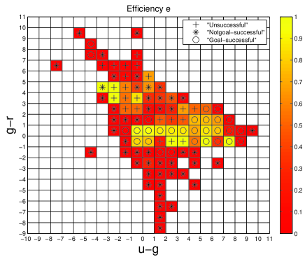
(a) Efficiency in $u-g$ vs $g-r$ plane for all clusters

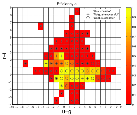
(b) Efficiency in $u-g$ vs $r-i$ plane for all clusters

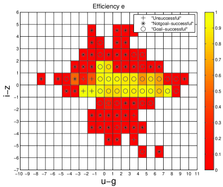
(c) Efficiency in $u-g$ vs $i-z$ plane for all clusters

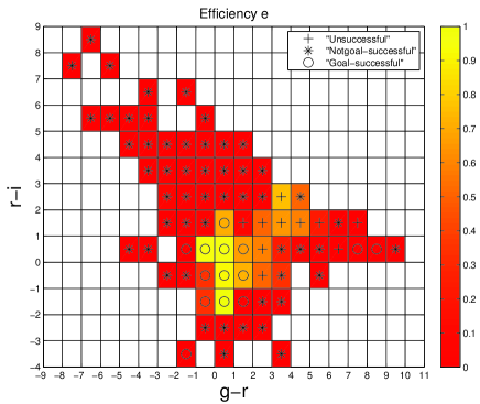
(d) Efficiency in $g-r$ vs $r-i$ plane for all clusters

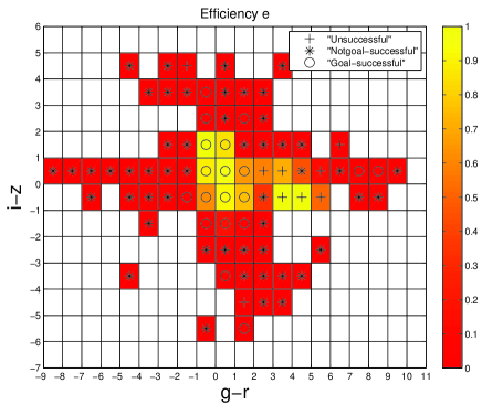
(e) Efficiency in $g-r$ vs $i-z$ plane for all clusters

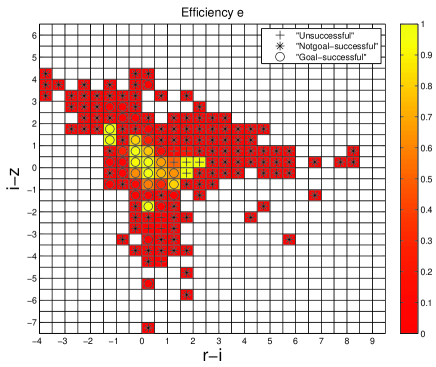
(f) Efficiency in $r-i$ vs $i-z$ plane for all clusters

Figure 34: Local efficiency estimates in the colour vs colour planes for the all types of clusters of experiment S-SCat.

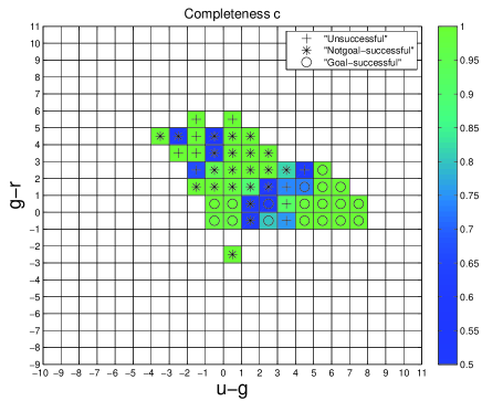
(a) Completeness in $u-g$ vs $g-r$ plane for all clusters

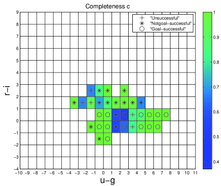
(b) Completeness in $u-g$ vs $r-i$ plane for all clusters

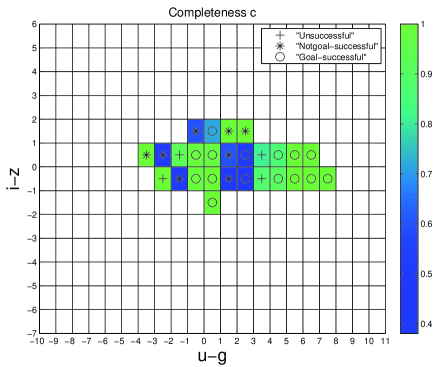
(c) Completeness in $u-g$ vs $i-z$ plane for all clusters

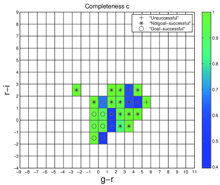
(d) Completeness in $g-r$ vs $r-i$ plane for all clusters

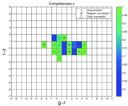
(e) Completeness in $g-r$ vs $i-z$ plane for all clusters

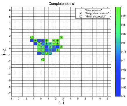
(f) Completeness in $r-i$ vs $i-z$ plane for all clusters

Figure 35: Local completeness estimates in the colour vs colour planes for the all types of clusters of experiment S-SCat.

7.3 The catalogue

A catalogue of QSO candidates has been extracted from the SDSS DR7 photometric catalogue using ”Method III”, described in section (4.5.3) and based on the application of the Mahalanobis’ distance to the distribution of photometric sources in the colour space and on the results of the experiment S-SCat. The total number of members of the catalogue of QSO candidates is $\sim 1,120,000$, which is in good agreement with the number of candidate quasars found in [Richards et al. 2008]. The general efficiency and completeness of the candidate QSOs selection process are 92$\%$ and 93$\%$ respectively, evaluated according to the method described in paragraph (4.4). The catalogue of candidate QSOs, for consistency with the SDSS footprint organization, has been splitted in several files, each corresponding to a different SDSS stripe of the observed sky. In the SDSS jargon, a stripe is defined by a line of constant survey latitude $\eta$, bounded on the north and south by the edges of the two strips (scans along a constant $\eta$ value), and bounded on the east and west by lines of constant lambda. Because both strips and stripes are defined in ”observed” space, they are rectangular areas which overlap as one approaches the poles (for more details see the web-page http://www.sdss.org). These files can be downloaded at the URL http://voneural.na.infn.it/qso.html as FITS files. Each file contains the fundamental SDSS parameters of the sources selected as candidates in the format listed in table (7).

Table 7: Format of the catalogues of QSOs candidates.

Column	Format	Description
1	I7	Unique catalogue number
2	A19	SDSS Object ID
3	F12.7	Right Ascension in deg (J2000)
4	F11.7	Declination in deg (J2000)
5	F7.3	$u$ psf dereddened magnitude
6	F6.3	$g$ psf dereddened magnitude
7	F6.3	$r$ psf dereddened magnitude
8	F6.3	$i$ psf dereddened magnitude
9	F6.3	$z$ psf dereddened magnitude
10	I7	”Goal-successful” cluster index

7.4 Comparison with the literature

The catalogue of QSO candidates here discussed is composed by stellar sources which have been selected because associated, in the parameter space, to one the ”goal-successful” clusters produced during the S-SCat experiment. In order to assess the validity of the extraction process against other catalogues of candidate quasars already available in the literature, we have crossmatched our catalogue with the ”NBC Quasar Candidate Catalog”, consisting of 100,563 unresolved, UV-excess (UVX) quasar candidates with magnitudes as faint as 21 in the $g$ band from 2099 square degrees of the SDSS DR1 imaging data (see [Richards et al. 2004]). This catalogue, extracted using the KDE method described in some details in paragraph (3.2) (the same method applied recently applied to the SDSS DR6 imaging data for the extraction of a larger catalogue of candidates not yet publicly available, see [Richards et al. 2008]), has been cross-matched with our catalogue of candidate quasars. The comparison of these two catalogues, even if the limiting magnitudes and covered areas of the photometric observations from which the candidates have been extractred are different, shows that less than $1\%$ of the candidates located in the overlapping regions of the sky and belonging to the KDE catalogue are not found inside our catalogue, while there is a $\sim 3\%$ of our candidates (once the same photometric cuts have been applied to the catalogues) which do not match any source listed in the KDE catalogue.

7.5 Number counts

Even though the efficiency and completeness of our photometrically selected sample of candidate QSOs are not unitary, the number count distribution of QSO candidates can be determined and used to characterize the candidates distribution in luminosity and for further comparison with other catalogues of QSOs candidate available in the literature.

The number counts (NC) of our candidates have been calculated in the redshift interval $0.3<z<2.2$. The sample of candidates used for the NC is formed only by those sources belonging to the ”goal-successful” clusters 1, 2 and 9 since, as can be noticed in the figure (28) and is pointed out in the description of the clusters in paragraph (7.2), such clusters are formed by groups of sources located at redshifts lower than 2.2. Selecting QSOs candidates in redshift by distinct clusters in the parameter space is reasonable since such clusters, formed by sources belonging to the BoK used for the esperiment, are clearly separated in redshift and the photometric QSOs candidates are expected to reflect the same partition along the redshift axis. In order to obtain an estimate of the NC in the $i$ band (figure 36), the efficiency e($i$) and completeness c($i$) have been used to correct for the performances of the selection process according to the following recipe. $N_{cat}(i)$, the density of candidates extracted from the catalogue in the generic magnitude interval $[i,i+di]$, is multiplied and divided by the efficiency e($i$) and completeness c($i$) respectively, measured in the same magnitude interval and yielding the corrected NC density $N(i)=N_{cat}(i)\cdot e(i)/c(i)$. Our NC estimates (diamonds in 36) are in fair agreement with the reference NC derived from the catalogue of candidate quasars produced using the KDE method in [Richards et al. 2008] (open squares). The error bars represent poissonian errors on the data points.

Figure 36: Number counts of quasars candidates in the SDSS $i$ band. Diamonds indicate the number counts of our candidates while the squares represent the number counts obtained in the same SDSS $i$ band using the quasar candidates extracted from a reference catalogue of candidate QSOs.

8 Discussion and conclusions

We have presented a new unsupervised method to perform quasar candidate selection, based on the clustering of astronomical sources in the parametric space defined by the photometric colours. The method requires a suitably large base of knowledge (BoK) which is used only for labelling purposes. The method consists of three steps: i) an unsupervised clustering performed by Probabilistic Principal Surfaces algorithm; ii) an agglomerative process driven by a measure of negative entropy, and iii) a fine tuning of the clustering performances through the exploitation of the information contained in the BoK. In the experiments described here, the BoK consists of the spectroscopic classification provided by the ”specClass” SDSS flag which is available for a relatively small fraction of the photometric sources observed by SDSS. Extensive testing on different data sets and parameter combinations and the comparison of the performance obtained in this experiments with the performance of the methods found in the literature and based on other techniques have shown that this method, which is based on a completely data-mining ground and employs tools never applied before to astronomical problems, can achieve better performances than most methods published in the literature so far (see section (5). The method has also been applied to the SDSS-DR7 data sets using the results of a specific experiment (S-SCat) and a catalogue of QSO candidates has been produced. This catalogue is publicly available at the web page http://voneural.na.infn.it/qso.html. Even though the method of unsupervised clustering in astronomical parameter spaces described in this paper has been adjusted to the case of SDSS QSOs selection, such fine tuning depends only on the information contained in the BoK and it can be applied to any similar case provided that a suitably large and complete base of knowledge is available. In this context, the role played by the Virtual Observatory for the future evolution of the data mining approach to classification/selection problems in astronomy, will be extremely important because the VO will allow the construction of BoKs of unprecedented accuracy and completeness obtained by federating and standardizing the information contained in most (if not all) astronomical databases worldwide, thus providing the most natural environment for the further development and exploitation of similar techniques.

Acknowledgements: This work was funded through the Ph.D. program of the University Federico II in Napoli, the European VOTECH consortium and the PON-SCOPE (financed by the Italian MIUR) and the italian Ministry of Foreign Affairs in the framework of the bilateral Italy-Usa agreement. R.D’A. acknowledges the Marie Curie EARA-EST action for financial support during his visit at the Institute of Astronomy, Cambridge (UK). The authors are grateful to the anonymous referee for useful suggestions that greatly helped to improve the paper. The authors also wish to thank M. Brescia, S. Cavuoti, E. De Filippis, O. Laurino, M. Paolillo and D. Capozzi for many useful discussions. A special thank goes to A. Staiano and A. Ciaramella for making available to us their implementations of the PPS and NEC algorithms.

Appendix A Local estimates of the efficiency and completeness

In this appendix, the plots of the local estimates of the efficiency $e$ and the completeness $c$ in the planes determined by the redshift and each photometric parameter (i.e., each colour) are shown for all the experiments described in the paper. Figure (37) represents the first experiment, while figures (38) and (39) describe the second experiment, and the remaining figures (40) and (41) are associated to the third and fourth experiments, respectively.

(a) Efficiency in $z$ vs $u-g$ plane

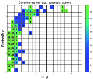
(b) Completeness in $z$ vs $u-g$ plane

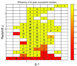
(c) Efficiency in $z$ vs $g-r$ plane

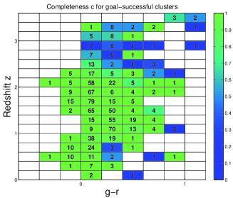
(d) Completeness in $z$ vs $g-r$ plane

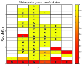
(e) Efficiency in $z$ vs $r-i$ plane

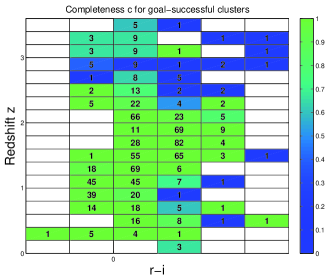
(f) Completeness in $z$ vs $r-i$ plane

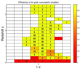
(g) Efficiency in $z$ vs $i-z$ plane

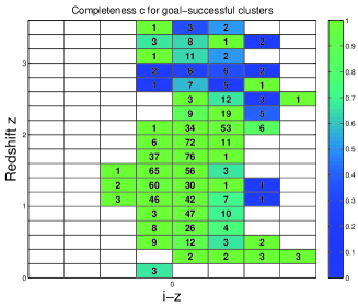
(h) Completeness in $z$ vs $i-z$ plane

Figure 37: Local efficiency (left-hand panels) and completeness (right-hand panels) estimates in the redshift vs optical colours planes for the labelling phase of the first experiment. Colour of the cell is associated to the efficiency and completeness of the selection process of the ”goal-successful” clusters, while numbers contained in each cell represent the total number of candidates in that region of the plane. Lower left-hand and right hand panels contain the maximum efficiency and completeness for the selection process of the three types of clusters produced by the algorithm. The class of clusters contributing the maximum fraction to the efficiency and completeness represented by the symbol contained in each cell of the plane.

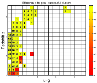
(a) Efficiency in $z$ vs $u-g$ plane

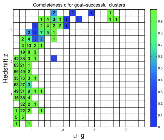
(b) Completeness in $z$ vs $u-g$ plane

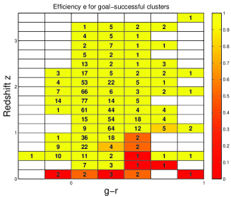
(c) Efficiency in $z$ vs $g-r$ plane

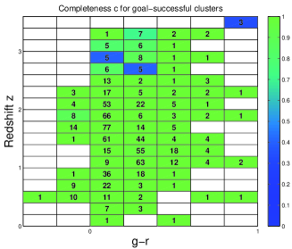
(d) Completeness in $z$ vs $g-r$ plane

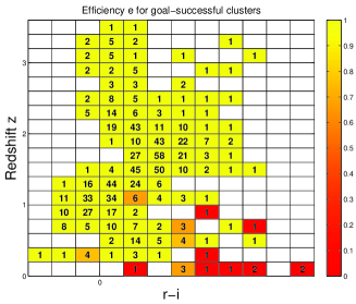
(e) Efficiency in $z$ vs $r-i$ plane

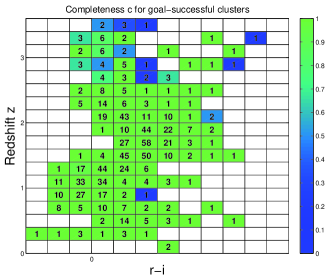
(f) Completeness in $z$ vs $r-i$ plane

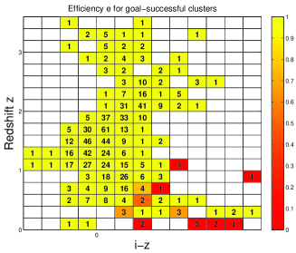
(g) Efficiency in $z$ vs $i-z$ plane

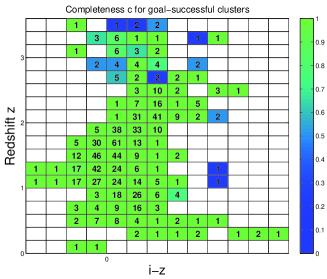
(h) Completeness in $z$ vs $i-z$ plane

Figure 38: Local efficiency and completeness for the second experiment (optical colours). See previous figure for details.

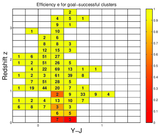
(a) Efficiency in $z$ vs $Y-J$ plane

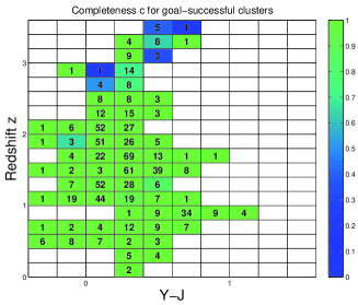
(b) Completeness in $z$ vs $Y-J$ plane

(c) Efficiency in $z$ vs $J-H$ plane

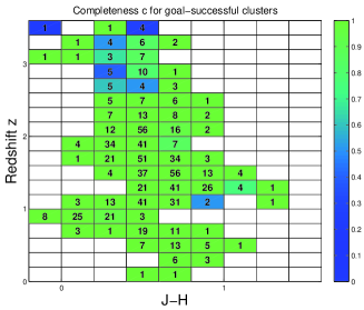
(d) Completeness in $z$ vs $J-H$ plane

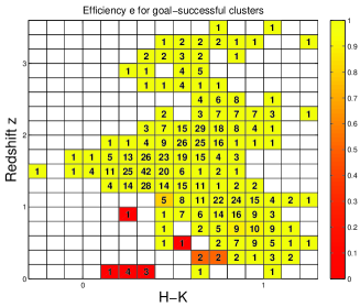
(e) Efficiency in $z$ vs $H-K$ plane

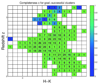
(f) Completeness in $z$ vs $H-K$ plane

Figure 39: Local efficiency and completeness for the second experiment (infrared colours).

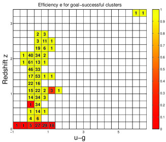
(a) Efficiency in $z$ vs $u-g$ plane

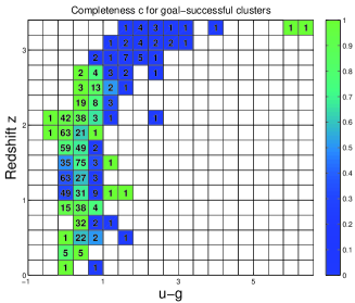
(b) Completeness in $z$ vs $u-g$ plane

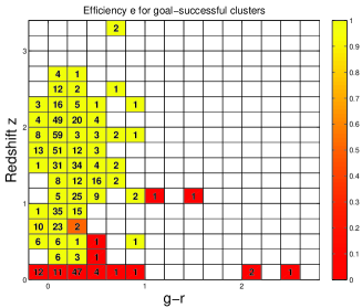
(c) Efficiency in $z$ vs $g-r$ plane

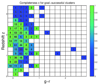
(d) Completeness in $z$ vs $g-r$ plane

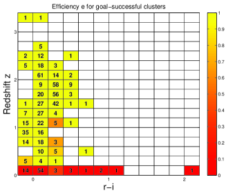
(e) Efficiency in $z$ vs $r-i$ plane

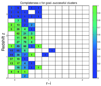
(f) Completeness in $z$ vs $r-i$ plane

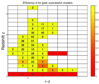
(g) Efficiency in $z$ vs $i-z$ plane

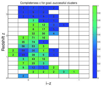
(h) Completeness in $z$ vs $i-z$ plane

Figure 40: Local efficiency and completeness for the third experiment.

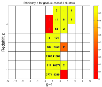
(a) Efficiency in $z$ vs $u-g$ plane

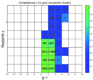
(b) Completeness in $z$ vs $u-g$ plane

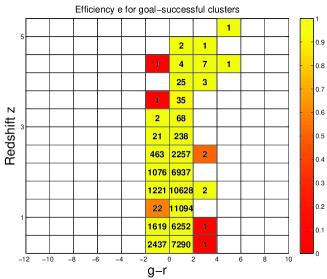
(c) Efficiency in $z$ vs $g-r$ plane

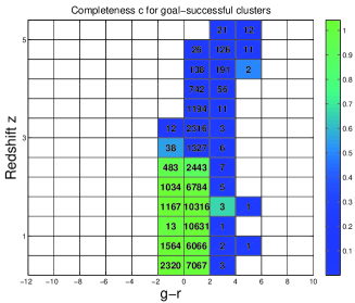
(d) Completeness in $z$ vs $g-r$ plane

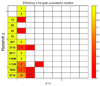
(e) Efficiency in $z$ vs $r-i$ plane

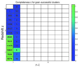
(f) Completeness in $z$ vs $r-i$ plane

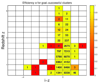
(g) Efficiency in $z$ vs $i-z$ plane

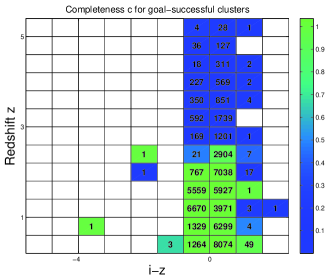
(h) Completeness in $z$ vs $i-z$ plane

Figure 41: Local efficiency and completeness for the fourth experiment.

References

- [Abazajian et al. 2008] Abazajian, K. et al., submitted to MNRAS.
- [Adelman et al. 2007] Adelman-McCarthy, J. K. et al. 2007, ApJS, 175, 297-313.
- [Bishop 1995] Bishop, C. M., Neural Networks for Pattern Recognition, Oxford University Press, 1995
- [Bishop 1998] Bishop, C. M., Svensen, M. & Williams, C. K. I. 1998, Neural Computation, 215-234
- [Bishop 1999] Bishop, C. M., Latent variable models, in M. I. Jordan (Ed.), Learning in Graphical Models, MIT Press, 1999
- [Boyle et al. 2000] Boyle, B. J., et al. 2000, MNRAS, 317, 1014-1022.
- [Capaccioli et al. 2003] Capaccioli, M., Mancini, D. & Sedmak, G. 2003, Memorie della Societ Astronomica Italiana, 74, 450-+
- [Cavuoti et al., in prep.] Cavuoti, S., D’Abrusco, R. & Longo, G., in preparation.
- [Chang 2001] Chang, K. Y. & Ghosh, J., A unified Model for Probabilistic Principal Surfaces 2001, in IEE Transactions on Pattern Analysis and Machine intelligence, 23, 22-41
- [Chang 2000] Chang, K. Y., & Ghosh, J. 2000. Three-Dimensional Model-Based Object Recognition and Pose Estimation Using Probabilistic Principal Surfaces, in SPIE: Applications of Artificial Neural Networks in Image, 2000, 192-203
- [Ciaramella 2005] Ciaramella, A., Longo, G., Staiano, A. & Tagliaferri, R. 2005, in WIRN/NAIS 2005 Proceedings, 49-56
- [Croom et al. 2001] Croom, S.M., Smith, R. J., Boyle, B. J., Shanks, T., Loaring, N. S.,Miller, L., & Lewis, I. J. 2001, MNRAS, 322, L29
- [D’Abrusco et al. 2007] D’Abrusco, R. et al. 2007, ApJ, 632, 752
- [D’Abrusco et al., in prep.] D’Abrusco, R. et al., in preparation.
- [Dempster et al. 1977] Dempster, A.P., Laird, N.M. & Rubin, D.B. Maximum-Likelihood from Incomplete Data Via the EM Algorithm, J. Royal Statistical Soc., Vol. 39, NO. 1, 1977
- [Djorgovski et al. 2004] Djorgovski, S. G et al. 2004, Bullettin of American Astronomical Society, 36, 1487-+
- [Dye et al. 2006] Dye, S. et al. 2006, MNRAS, 372, 1227-1252
- [Fan et al. 2001b] Fan, X., et al., 2001b, AJ, 121, 54
- [Fan et al. 2006] Fan, X. 2006, AJ, 131, 1203.
- [Fukugita et al. 1996] Fukugita et al. 1996, AJ, 111, 1748-+
- [Hall et al. 1996] Hall, P. B., et al. 1996, ApJ, 462, 614-+
- [Hewitt et al. 1993] Hewitt, A. & Burbidge, G.R. 1993, ApJS, 87, 451
- [Hewett et al. 1995] Hewett, P. C., Foltz, C. B., & Chaffee, F. H. 1995, AJ, 109, 1498
- [Jarrett et al. 2000] Jarrett, T.H. et al. 2000, AJ, 119, 2498
- [Koo & Kron 1982] Koo, D. C. & Kron, R. G. 1988, ApJ, 325, 92
- [Lacy et al. 2004] Lacy, M. et al. 2004, ApJS, 154, 166.
- [Lawrence et al. 2007] Lawrence, A. et al. 2007, MNRAS, 379, 1599-1617
- [Lynds 1971] Lynds, R. 1971, ApJL, 164, L73+
- [McPherson et al. 2006] McPherson, A. M., Born, A. J., Sutherland, W. J. & Emerson, J. P. 2006, in ”Ground-based Telescopes”, Proceedings of the SPIE, 5489, 638-649
- [Richards et al. 2001] Richards, G. T. et al. 2001, AJ, 121, 2308-2330
- [Richards et al. 2002] Richards, G. T. et al. 2002, ApJ, 123, 2945
- [Richards et al. 2004] Richards, G. T. et al. 2004, ApJS, 155, 257-269.
- [Richards et al. 2008] Richards, G. T. et al. 2008, ApJS, 180, 67-83.
- [Sandage & Wyndham 1965] Sandage, A. & Wyndham, J.D. 1965, ApJ, 141, 328
- [Schmidt & Green 1983] Schmidt, M. & Green, R. F. 1983, ApJ, 269, 352
- [Schneider et al. 2007] Schneider, D. P. et al. 2007, AJ, 134, 102.
- [Staiano 2003] Staiano A., 2003, Unsupervised Neural Networks for the Extraction of Scientific Information from Astronomical Data, PhD thesis, University of Salerno
- [Staiano 2004] Staiano A., De Vinco L., Ciaramella A., Raiconi G., Tagliaferri R., Longo G., Miele G., Amato R., Del Mondo C., Donalek C., Mangano G., Di Bernardo D.: Probabilistic principal surfaces for yeast gene microarray data-mining, in ICDM’04 - Fourth IEEE International Conference on Data Mining, pp. 202-209, (2004)
- [Stern et al. 2005] Stern, D. et al. 2005, ApJ, 631, 163.
- [Stoughton et al. 2002] Stoughton, C. et al. 2002, AJ, 123, 485-548
- [Vanden Berk et al. 2005] Vanden Berk D. E. et al. 2005, AJ, 129, 2047-2061
- [Walton 2002] Walton, N. A. 2002, Astronomy and Geophysics, 43, 30-31
- [Warren & Hewett 1990] Warren, S. J. & Hewett, P. C. 1990, Rep. Prog. Phys., 53, 1095
- [Warren et al. 1991] Warren, S. J., Hewett, P. C., & Osmer, P. S. 1991, ApJS, 76, 23
- [Warren et al. 2000] Warren, S. J., Hewett, P. C., & Foltz, C. B. 2000, MNRAS, 312, 827-832.
- [York et al. 2000] York, D. G. et al. 2000, AJ, 120, 1279-1587.