Chaotic Spin Dynamics of a Long Nanomagnet Driven by a Current

Abstract.

We study the spin dynamics of a long nanomagnet driven by an electrical current. In the case of only DC current, the spin dynamics has a sophisticated bifurcation diagram of attractors. One type of attractors is a weak chaos. On the other hand, in the case of only AC current, the spin dynamics has a rather simple bifurcation diagram of attractors. That is, for small Gilbert damping, when the AC current is below a critical value, the attractor is a limit cycle; above the critical value, the attractor is chaotic (turbulent). For normal Gilbert damping, the attractor is always a limit cycle in the physically interesting range of the AC current. We also developed a Melnikov integral theory for a theoretical prediction on the occurrence of chaos. Our Melnikov prediction seems performing quite well in the DC case. In the AC case, our Melnikov prediction seems predicting transient chaos. The sustained chaotic attractor seems to have extra support from parametric resonance leading to a turbulent state.

1. Introduction

The greatest potential of the theory of chaos in partial differential equations lies in its abundant applications in science and engineering. The variety of the specific problems demands continuing innovation of the theory [17] [16] [18] [23] [24] [15] [20] [21]. In these representative publications, two theories were developed. The theory developed in [17] [16] [18] involves transversal homoclinic orbits, and shadowing technique is used to prove the existence of chaos. This theory is very complete. The theory in [23] [24] [15] [20] [21] deals with Silnikov homoclinic orbits, and geometric construction of Smale horseshoes is employed. This theory is not very complete. The main machineries for locating homoclinic orbits are (1). Darboux transformations, (2). Isospectral theory, (3). Persistence of invariant manifolds and Fenichel fibers, (4). Melnikov analysis and shooting technique. Overall, the two theories on chaos in partial differential equations are results of combining Integrable Theory, Dynamical System Theory, and Partial Differential Equations [19].

In this article, we are interested in the chaotic spin dynamics in a long nanomagnet diven by an electrical current. We hope that the abundant spin dynamics revealed by this study can generate experimental studies on long nanomagets. To illustrate the general significance of the spin dynamics, in particular the magnetization reversal issue, we use a daily example: The memory of the hard drive of a computer. The magnetization is polarized along the direction of the external magnetic field. By reversing the external magnetic field, magnetization reversal can be accomplished; thereby, generating $0$ and $1$ binary sequence and accomplishing memory purpose. Memory capacity and speed via such a technique have reached their limits. The “bit” writing scheme based on such Oersted-Maxwell magnetic field (generated by an electrical current) encounters fundamental problem from classical electromagnetism: the long range magnetic field leads to unwanted writing or erasing of closely packed neighboring magnetic elements in the extremely high density memory device and the induction laws place an upper limit on the memory speed due to slow rise-and-decay-time imposed by the law of induction. Discovered by Slonczewski [35] and Berger [1], electrical current can directly apply a large torque to a ferromagnet. If electrical current can be directly applied to achieve magnetization reversal, such a technique will dramatically increase the memory capacity and speed of a hard drive. The magnetization can then be switched on the scale of nanoseconds and nanometers [39]. The industrial value will be tremendous. Nanomagnets driven by currents has been intensively studied recently [13, 10, 34, 7, 14, 12, 33, 8, 39, 11, 32, 37, 38, 4, 3, 26, 27, 29, 42, 31]. The researches have gone beyond the original spin valve system [35] [1]. For instance, current driven torques have been applied to magnetic tunnel junctions [36] [6], dilute magnetic semiconductors [40], multi-magnet couplings [10] [14]. AC currents were also applied to generate spin torque [34] [7]. Such AC current can be used to generate the external magnetic field [34] or applied directly to generate spin torque [7].

Mathematically, the electrical current introduces a spin torque forcing term in the conventional Landau-Lifshitz-Gilbert (LLG) equation. The AC current can induce novel dynamics of the LLG equation, like synchronization [34] [7] and chaos [25] [41]. Both synchronization and chaos are important phenomena to understand before implementing the memory technology. In [25] [41], we studied the dynamics of synchronization and chaos for the LLG equation by ignoring the exchange field (i.e. LLG ordinary differential equations). When the nanomagnetic device has the same order of length along every direction, exchange field is not important, and we have a so-called single domain situation where the spin dynamics is governed by the LLG ordinary differential equations. In this article, we will study what we call “long nanomagnet” which is much longer along one direction than other directions. In such a situation, the exchange field will be important. This leads to a LLG partial differential equation. In fact, we will study the case where the exchange field plays a dominant role.

The article is organized as follows: Section 2 presents the mathematical formulation of the problem. Section 3 is an integrable study on the Heisenberg equation. Based upon Section 3, Section 4 builds the Melnikov integral theory for predicting chaos. Section 5 presents the numerical simulations. Section 6 is an appendix to Section 3.

2. Mathematical Formulation

To simplify the study, we will investigate the case that the magnetization depends on only one spatial variable, and has periodic boundary condition in this spatial variable. The application of this situation will be a large ring shape nanomagnet. Thus, we shall study the following forced Landau-Lifshitz-Gilbert (LLG) equation in the dimensionless form,

(2.1) $$\partial_{t}m=-m\times H-\epsilon\alpha m\times(m\times H)+\epsilon(\beta_{1}+\beta_{2}\cos\omega_{0}t)m\times(m\times e_{x})\ ,$$

subject to the periodic boundary condition

(2.2) $$m(t,x+2\pi)=m(t,x)\ ,$$

where $m$ is a unit magnetization vector $m=(m_{1},m_{2},m_{3})$ in which the three components are along ($x,y,z$) directions with unit vectors ($e_{x},e_{y},e_{z}$), $|m|(t,x)=1$, the effective magnetic field $H$ has several terms

(2.3) $$H = H_{\mbox{exch}}+H_{\mbox{ext}}+H_{\mbox{dem}}+H_{\mbox{ani}}$$

$$= \partial_{x}^{2}m+\epsilon ae_{x}-\epsilon m_{3}e_{z}+\epsilon bm_{1}e_{x}\ ,$$

where $H_{\mbox{exch}}=\partial_{x}^{2}m$ is the exchange field, $H_{\mbox{ext}}=\epsilon ae_{x}$ is the external field, $H_{\mbox{dem}}=-\epsilon m_{3}e_{z}$ is the demagnetization field, and $H_{\mbox{ani}}=\epsilon bm_{1}e_{x}$ is the anisotropy field. For the materials of the experimental interest, the dimensionless parameters are in the ranges

$$a\approx 0.05\ ,\quad b\approx 0.025\ ,\quad\alpha\approx 0.02\ ,$$

(2.4) $$\beta_{1}\in[0.01,0.3]\ ,\quad\beta_{2}\in[0.01,0.3]\ ;$$

and $\epsilon$ is a small parameter measuring the length scale of the exchange field. One can also add an AC current effect in the external field $H_{\mbox{ext}}$, but the results on the dynamics are similar.

Our goal is to build a Melnikov function for the LLG equation around domain walls. The roots of such a Melnikov function provide a good indication of chaos.

For the rest of this section, we will introduce a few interesting notations. The Pauli matrices are:

(2.5) $$\sigma_{1}=\left(\begin{array}[]{lr}0&1\cr 1&0\cr\end{array}\right)\ ,\quad\sigma_{2}=\left(\begin{array}[]{lr}0&-i\cr i&0\cr\end{array}\right)\ ,\quad\sigma_{3}=\left(\begin{array}[]{lr}1&0\cr 0&-1\cr\end{array}\right)\ .$$

Let

(2.6) $$m_{+}=m_{1}+im_{2}\ ,\quad m_{-}=m_{1}-im_{2}\ ,$$

i.e. $\overline{m_{+}}=m_{-}$. Let

(2.7) $$\Gamma=m_{j}\sigma_{j}=\left(\begin{array}[]{lr}m_{3}&m_{-}\cr m_{+}&-m_{3}\cr\end{array}\right)\ .$$

Thus, $\Gamma^{2}=I$ (the identity matrix). Let

$$\hat{H}=-H-\alpha m\times H+\beta m\times e_{x}\ ,\quad\Pi=\left(\begin{array}[]{lr}\hat{H}_{3}&\hat{H}_{1}-i\hat{H}_{2}\cr\hat{H}_{1}+i\hat{H}_{2}&-\hat{H}_{3}\cr\end{array}\right)\ .$$

Then the LLG can be written in the form

(2.8) $$i\partial_{t}\Gamma=\frac{1}{2}[\Gamma,\Pi]\ ,$$

where $[\Gamma,\Pi]=\Gamma\Pi-\Pi\Gamma$.

3. Isospectral Integrable Theory for the Heisenberg Equation

Setting $\epsilon$ to zero, the LLG (2.1) reduces to the Heisenberg ferromagnet equation,

(3.1) $$\partial_{t}m=-m\times m_{xx}\ .$$

Using the matrix $\Gamma$ introduced in (2.7), the Heisenberg equation (3.1) has the form

(3.2) $$i\partial_{t}\Gamma=-\frac{1}{2}[\Gamma,\Gamma_{xx}]\ ,$$

where the bracket $[\ ,\ ]$ is defined in (2.8). Obvious constants of motion of the Heisenberg equation (3.1) are the Hamiltonian,

$$\frac{1}{2}\int_{0}^{2\pi}|m_{x}|^{2}dx\ ,$$

the momentum,

$$\int_{0}^{2\pi}\frac{m_{1}m_{2x}-m_{2}m_{1x}}{1+m_{3}}dx\ ,$$

and the total spin,

$$\int_{0}^{2\pi}mdx\ .$$

The Heisenberg equation (3.1) is an integrable system with the following Lax pair,

(3.3) $$\partial_{x}\psi = i\lambda\Gamma\psi\ ,$$

(3.4) $$\partial_{t}\psi = -\frac{\lambda}{2}\left(4i\lambda\Gamma+[\Gamma,\Gamma_{x}]\right)\psi\ ,$$

where $\psi=(\psi_{1},\psi_{2})^{T}$ is complex-valued, $\lambda$ is a complex parameter, $\Gamma$ is the matrix defined in (2.7), and $[\Gamma,\Gamma_{x}]=\Gamma\Gamma_{x}-\Gamma_{x}\Gamma$. In fact, there is a connection between the Heisenberg equation (3.1) and the 1D integrable focusing cubic nonlinear Schrödinger (NLS) equation via a nontrivial gauge transformation. The details of this connection are given in the Appendix.

3.1. A Simple Linear Stability Calculation

As shown in the Appendix, the temporally periodic solutions of the NLS equation correspond to the domain walls of the Heisenberg equation. Consider the domain wall

$$\Gamma_{0}=\left(\begin{array}[]{lr}0&e^{-i\xi x}\cr e^{i\xi x}&0\cr\end{array}\right),\ \xi\in\mathbb{Z};\quad\mbox{i.e.}\ m_{1}=\cos\xi x,\ m_{2}=\sin\xi x,\ m_{3}=0,$$

which is a fixed point of the Heisenberg equation. Linearizing the Heisenberg equation at this fixed point, one gets

$$i\partial_{t}\Gamma=-\frac{1}{2}[\Gamma_{0},\Gamma_{xx}]-\frac{1}{2}[\Gamma,\Gamma_{0xx}]\ .$$

Let

$$\Gamma=\left(\begin{array}[]{lr}m_{3}&e^{-i\xi x}(m_{1}-im_{2})\cr e^{i\xi x}(m_{1}+im_{2})&-m_{3}\cr\end{array}\right)\ ,$$

we get

$$\partial_{t}m_{1}=0\ ,\quad\partial_{t}m_{2}=m_{3xx}+\xi^{2}m_{3}\ ,\quad\partial_{t}m_{3}=-m_{2xx}-2\xi m_{1x}\ .$$

Let

$$m_{j}=\sum_{k=0}^{\infty}(m_{jk}^{+}(t)\cos kx+m_{jk}^{-}(t)\sin kx)\ ,$$

where $m_{jk}^{\pm}(t)=c_{jk}^{\pm}e^{\Omega t}$, $c_{jk}^{\pm}$ and $\Omega$ are constants. We obtain that

(3.5) $$\Omega=\sqrt{k^{2}(\xi^{2}-k^{2})}$$

which shows that only the modes $0<|k|<|\xi|$ are unstable. Such instability is called a modulational instability, also called a side-band instability. Comparing the Heisenberg ferromagnet equation (3.1) and the Landau-Lifshitz-Gilbert equation (2.1), we see that if we drop the exchange field $H_{\mbox{exch}}=\partial_{x}^{2}m$ in the effective magnetic field $H$ (2.3), such a modulational instability will disappear, and the Landau-Lifshitz-Gilbert equation (2.1) reduces to a system of three ordinary differential equations, which has no chaos as verified numerically. Thus the modulational instability is the source of the chaotic magnetization dynamics.

In terms of $m_{jk}^{\pm}$, we have

$$\frac{d}{dt}m_{1k}^{\pm}=0,\ \frac{d}{dt}m_{2k}^{\pm}=(\xi^{2}-k^{2})m_{3k}^{\pm},\ \frac{d}{dt}m_{3k}^{\pm}=k^{2}m_{2k}^{\pm}\mp 2\xi km_{1k}^{\mp}.$$

Choosing $\xi=2$, we have for $k=0$,

$$\left(\begin{array}[]{c}m_{10}^{\mp}\cr m_{20}^{\pm}\cr m_{30}^{\pm}\cr\end{array}\right)=c_{1}\left(\begin{array}[]{c}1\cr 0\cr 0\cr\end{array}\right)+c_{2}\left(\begin{array}[]{c}0\cr 1\cr 0\cr\end{array}\right)+c_{3}\left(\begin{array}[]{c}0\cr 4t\cr 1\cr\end{array}\right)\ ;$$

for $k=1$,

$$\left(\begin{array}[]{c}m_{11}^{\mp}\cr m_{21}^{\pm}\cr m_{31}^{\pm}\cr\end{array}\right)=c_{1}\left(\begin{array}[]{c}1\cr\pm 4\cr 0\cr\end{array}\right)+c_{2}\left(\begin{array}[]{c}0\cr\sqrt{3}\cr 1\cr\end{array}\right)e^{\sqrt{3}t}+c_{3}\left(\begin{array}[]{c}0\cr-\sqrt{3}\cr 1\cr\end{array}\right)e^{-\sqrt{3}t}\ ;$$

for $k=2$,

$$\left(\begin{array}[]{c}m_{12}^{\mp}\cr m_{22}^{\pm}\cr m_{32}^{\pm}\cr\end{array}\right)=c_{1}\left(\begin{array}[]{c}0\cr 0\cr 1\cr\end{array}\right)+c_{2}\left(\begin{array}[]{c}1\cr 0\cr\mp 8t\cr\end{array}\right)+c_{3}\left(\begin{array}[]{c}0\cr 1\cr 4t\cr\end{array}\right)\ ;$$

for $k>2$,

$$\left(\begin{array}[]{c}m_{1k}^{\mp}\cr m_{2k}^{\pm}\cr m_{3k}^{\pm}\cr\end{array}\right) = c_{1}\left(\begin{array}[]{c}1\cr\pm 4/k\cr 0\cr\end{array}\right)+c_{2}\left(\begin{array}[]{c}0\cr\sqrt{k^{2}-4}\cos(k\sqrt{k^{2}-4}t)\cr k\sin(k\sqrt{k^{2}-4}t)\cr\end{array}\right)$$

$$+c_{3}\left(\begin{array}[]{c}0\cr-\sqrt{k^{2}-4}\sin(k\sqrt{k^{2}-4}t)\cr k\cos(k\sqrt{k^{2}-4}t)\cr\end{array}\right)\ ;$$

where $c_{1}$, $c_{2}$ and $c_{3}$ are arbitrary constants.

The nonlinear foliation of the above linear modulational instability can be established via a Darboux transformation.

3.2. A Darboux Transformation

A Darboux transformation for (3.3)-(3.4) can be obtained.

Theorem 3.1.

Let $\phi=(\phi_{1},\phi_{2})^{T}$ be a solution to the Lax pair (3.3)-(3.4) at ($\Gamma,\nu$). Define the matrix

$$G=N\left(\begin{array}[]{cc}(\nu-\lambda)/\nu&0\cr 0&(\bar{\nu}-\lambda)/\bar{\nu}\cr\end{array}\right)N^{-1}\ ,$$

where

$$N=\left(\begin{array}[]{lr}\phi_{1}&-\overline{\phi_{2}}\cr\phi_{2}&\overline{\phi_{1}}\cr\end{array}\right)\ .$$

Then if $\psi$ solves the Lax pair (3.3)-(3.4) at ($\Gamma,\lambda$),

(3.8) $$\hat{\psi}=G\psi$$

solves the Lax pair (3.3)-(3.4) at ($\hat{\Gamma},\lambda$), where $\hat{\Gamma}$ is given by

(3.9) $$\hat{\Gamma}=N\left(\begin{array}[]{lr}e^{-i\theta}&0\cr 0&e^{i\theta}\cr\end{array}\right)N^{-1}\Gamma N\left(\begin{array}[]{lr}e^{i\theta}&0\cr 0&e^{-i\theta}\cr\end{array}\right)N^{-1}\ ,$$

where $e^{i\theta}=\nu/|\nu|$.

The transformation (3.8)-(3.9) is called a Darboux transformation. This theorem can be proved either through the connection between the Heisenberg equation and the NLS equation (with a well-known Darboux transformation) [2], or through a direct calculation.

Notice also that $\hat{\Gamma}^{2}=I$. Let

(3.14) $$\left(\begin{array}[]{lr}\Phi_{1}&-\overline{\Phi_{2}}\cr\Phi_{2}&\overline{\Phi_{1}}\cr\end{array}\right)=N\left(\begin{array}[]{lr}e^{-i\theta}&0\cr 0&e^{i\theta}\cr\end{array}\right)N^{-1}$$

(3.17) $$=\frac{1}{|\phi_{1}|^{2}+|\phi_{2}|^{2}}\left(\begin{array}[]{lr}e^{-i\theta}|\phi_{1}|^{2}+e^{i\theta}|\phi_{2}|^{2}&-2i\sin\theta\ \phi_{1}\overline{\phi_{2}}\cr-2i\sin\theta\ \overline{\phi_{1}}\phi_{2}&e^{i\theta}|\phi_{1}|^{2}+e^{-i\theta}|\phi_{2}|^{2}\cr\end{array}\right)\ .$$

Then

(3.18) $$\hat{\Gamma}=\left(\begin{array}[]{lr}\hat{m}_{3}&\hat{m}_{1}-i\hat{m}_{2}\cr\hat{m}_{1}+i\hat{m}_{2}&-\hat{m}_{3}\cr\end{array}\right)\ ,$$

where

$$\hat{m}_{+}=\hat{m}_{1}+i\hat{m}_{2}=\overline{\Phi_{1}}^{2}(m_{1}+im_{2})-\Phi_{2}^{2}(m_{1}-im_{2})+2\overline{\Phi_{1}}\Phi_{2}m_{3}\ ,$$

$$\hat{m}_{3}=\left(|\Phi_{1}|^{2}-|\Phi_{2}|^{2}\right)m_{3}-\overline{\Phi_{1}}\overline{\Phi_{2}}(m_{1}+im_{2})-\Phi_{1}\Phi_{2}(m_{1}-im_{2})\ .$$

One can generate the figure eight connecting to the domain wall, as the nonlinear foliation of the modulational instability, via the above Darboux transfomation.

3.3. Figure Eight Connecting to the Domain Wall

Let $\Gamma$ be the domain wall

$$\Gamma=\left(\begin{array}[]{lr}0&e^{-i2x}\cr e^{i2x}&0\cr\end{array}\right)\ ,$$

i.e. $m_{1}=\cos 2x$, $m_{2}=\sin 2x$, and $m_{3}=0$. Solving the Lax pair (3.3)-(3.4), one gets two Bloch eigenfunctions

(3.19) $$\psi=e^{\Omega t}\left(\begin{array}[]{c}2\lambda\exp\{\frac{i}{2}(k-2)x\}\cr(k-2)\exp\{\frac{i}{2}(k+2)x\}\cr\end{array}\right)\ ,\quad\Omega=-i\lambda k\ ,\quad k=\pm 2\sqrt{1+\lambda^{2}}\ .$$

To apply the Darboux transformation (3.9), we start with the two Bloch functions with $k=\pm 1$,

(3.22) $$\phi^{+} = \left(\begin{array}[]{c}\sqrt{3}e^{-ix}\cr ie^{ix}\cr\end{array}\right)\exp\left\{\frac{\sqrt{3}}{2}t+i\frac{1}{2}x\right\}\ ,$$

(3.26) $$\phi^{-} = \left(\begin{array}[]{c}-ie^{-ix}\cr\sqrt{3}e^{ix}\cr\end{array}\right)\exp\left\{-\frac{\sqrt{3}}{2}t-i\frac{1}{2}x\right\}\ .$$

The wise choice for $\phi$ used in (3.9) is:

(3.27) $$\phi=\sqrt{\frac{c^{+}}{c^{-}}}\phi^{+}+\sqrt{\frac{c^{-}}{c^{+}}}\phi^{-}=\left(\begin{array}[]{c}\left(\sqrt{3}e^{\tau+i\chi}-ie^{-\tau-i\chi}\right)e^{-ix}\cr\left(ie^{\tau+i\chi}+\sqrt{3}e^{-\tau-i\chi}\right)e^{ix}\cr\end{array}\right)\ ,$$

where $c^{+}/c^{-}=\exp\{\sigma+i\gamma\}$, $\tau=\frac{1}{2}(\sqrt{3}t+\sigma)$, and $\chi=\frac{1}{2}(x+\gamma)$. Then from the Darboux transformation (3.9), one gets

(3.28) $$\hat{m}_{1}+i\hat{m}_{2} = -e^{i2x}\bigg{\{}1-\frac{2\ \mbox{sech}2\tau\cos 2\chi}{(2-\sqrt{3}\ \mbox{sech}2\tau\sin 2\chi)^{2}}\bigg{[}\ \mbox{sech}2\tau\cos 2\chi$$

$$+i\left(\sqrt{3}-2\ \mbox{sech}2\tau\sin 2\chi\right)\bigg{]}\bigg{\}}\ ,$$

(3.29) $$\hat{m}_{3} = \frac{2\ \mbox{sech}2\tau\tanh 2\tau\cos 2\chi}{(2-\sqrt{3}\ \mbox{sech}2\tau\sin 2\chi)^{2}}\ .$$

As $t\rightarrow\pm\infty$,

$$\hat{m}_{1}\rightarrow-\cos 2x\ ,\quad\hat{m}_{2}\rightarrow-\sin 2x\ ,\quad\hat{m}_{3}\rightarrow 0\ .$$

The expressions (3.28)-(3.29) represent the two dimensional figure eight separatrix connecting to the domain wall ($m_{+}=-e^{i2x}$, $m_{3}=0$), parametrized by $\sigma$ and $\gamma$. See Figure 1 for an illustration. Choosing $\gamma=0,\pi$, one gets the figure eight curve section of Figure 1. The spatial-temporal profiles corresponding to the two lobes of the figure eight curve are shown in Figure 2. In fact, the two profiles corresponding the two lobes are spatial translates of each other by $\pi$. Inside one of the lobe, the spatial-temporal profile is shown in Figure 3(a). Outside the figure eight curve, the spatial-temporal profile is shown in Figure 3(b). Here the inside and outside spatial-temporal profiles are calculated by using the integrable finite difference discretization [9] of the Heisenberg equation (3.1),

(3.30) $$\frac{d}{dt}m(j)=-\frac{2}{h^{2}}m(j)\times\left(\frac{m(j+1)}{1+m(j)\cdot m(j+1)}+\frac{m(j-1)}{1+m(j-1)\cdot m(j)}\right),$$

where $m(j)=m(t,jh)$, $j=1,\cdots,N$, $Nh=2\pi$, and $h$ is the spatial mesh size. For the computation of Figure 3, we choose $N=128$.

Figure 1. The separatrix connecting to the domain wall $m_{+}=-e^{i2x},m_{3}=0$.

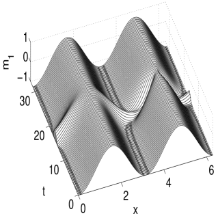
(a) $\gamma=0$

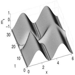
(b) $\gamma=\pi$

Figure 2. The spatial-temporal profiles corresponding to the two lobes of the figure eight curve.

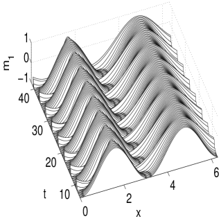
(a) inside

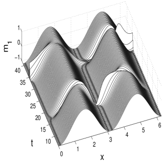
(b) outside

Figure 3. The spatial-temporal profiles corresponding to the inside and outside of the figure eight curve.

By a translation $x\rightarrow x+\theta$, one can generate a circle of domain walls:

$$m_{+}=-e^{i2(x+\theta)}\ ,\quad m_{3}=0\ ,$$

where $\theta$ is the phase parameter. The three dimensional figure eight separatrix connecting to the circle of domain walls, parametrized by $\sigma$, $\gamma$ and $\theta$; is illustrated in Figure 4.

In general, the unimodal equilibrium manifold can be sought as follows: Let

$$m_{j}=c_{j}\cos 2x+s_{j}\sin 2x\ ,\quad j=1,2,3,$$

then the uni-length condition $|m|(x)=1$ leads to

$$|c|=1\ ,\quad|s|=1\ ,\quad c\cdot s=0\ ,$$

where $c$ and $s$ are the two vectors with components $c_{j}$ and $s_{j}$. Thus the unimodal equilibrium manifold is three dimensional and can be represented as in Figure 5.

Using the formulae (3.28)-(3.29), we want to build a Melnikov integral. The zeros of the Melnikov integral will give a prediction on the existence of chaos. To build such a Melnikov integral, we need to first develop a Melnikov vector. This requires Floquet theory of (3.3).

Figure 4. The separatrix connecting to the circle of domain walls $m_{+}=e^{i2(x+\theta)},m_{3}=0$.

Figure 5. A representation of the 3 dimensional unimodal equilibrium manifold.

3.4. Floquet Theory

Focusing on the spatial part (3.3) of the Lax pair (3.3)-(3.4), let $Y(x)$ be the fundamental matrix solution of (3.3), $Y(0)=I$ ($2\times 2$ identity matrix), then the Floquet discriminant is defined by

$$\Delta=\ \mbox{trace}\ Y(2\pi)\ .$$

The Floquet spectrum is given by

$$\sigma=\{\lambda\in\mathbb{C}\ |\ -2\leq\Delta(\lambda)\leq 2\}\ .$$

Periodic and anti-periodic points $\lambda^{\pm}$ (which correspond to periodic and anti-periodic eigenfunctions respectively) are defined by

$$\Delta(\lambda^{\pm})=\pm 2\ .$$

A critical point $\lambda^{(c)}$ is defined by

$$\frac{d\Delta}{d\lambda}(\lambda^{(c)})=0\ .$$

A multiple point $\lambda^{(n)}$ is a periodic or anti-periodic point which is also a critical point. The algebraic multiplicity of $\lambda^{(n)}$ is defined as the order of the zero of $\Delta(\lambda)\pm 2$ at $\lambda^{(n)}$. When the order is $2$, we call the multiple point a double point, and denote it by $\lambda^{(d)}$. The order can exceed $2$. The geometric multiplicity of $\lambda^{(n)}$ is defined as the dimension of the periodic or anti-periodic eigenspace at $\lambda^{(n)}$, and is either $1$ or $2$.

Counting lemmas for $\lambda^{\pm}$ and $\lambda^{(c)}$ can be established as in [30] [23], which lead to the existence of the sequences $\{\lambda_{j}^{\pm}\}$ and $\{\lambda_{j}^{(c)}\}$ and their approximate locations. Nevertheless, counting lemmas are not necessary here. For any $\lambda\in\mathbb{C}$, $\Delta(\lambda)$ is a constant of motion of the Heisenberg equation (3.1). This is the so-called isospectral theory.

Example 3.2.

For the domain wall $m_{1}=\cos 2x$, $m_{2}=\sin 2x$, and $m_{3}=0$; the two Bloch eigenfunctions are given in (3.19). The Floquet discriminant is given by

$$\Delta=2\cos\left[2\pi\sqrt{1+\lambda^{2}}\right]\ .$$

The periodic points are given by

$$\lambda=\pm\sqrt{\frac{n^{2}}{4}-1}\ ,\quad n\in\mathbb{Z}\ ,\quad n\ \mbox{is even}\ .$$

The anti-periodic points are given by

$$\lambda=\pm\sqrt{\frac{n^{2}}{4}-1}\ ,\quad n\in\mathbb{Z}\ ,\quad n\ \mbox{is odd}\ .$$

The choice of $\phi^{+}$ and $\phi^{-}$ correspond to $n=\pm 1$ and $\lambda=\nu=i\sqrt{3}/2$ with $k=\pm 1$.

$$\Delta^{\prime}=-4\pi\frac{\lambda}{\sqrt{1+\lambda^{2}}}\sin\left[2\pi\sqrt{1+\lambda^{2}}\right]\ .$$

$$\Delta^{\prime\prime}=-4\pi(1+\lambda^{2})^{-3/2}\sin\left[2\pi\sqrt{1+\lambda^{2}}\right]-8\pi^{2}\frac{\lambda^{2}}{1+\lambda^{2}}\cos\left[2\pi\sqrt{1+\lambda^{2}}\right]\ .$$

When $n=0$, i.e. $\sqrt{1+\lambda^{2}}=0$, by L’Hospital’s rule

$$\Delta^{\prime}\rightarrow-8\pi^{2}\lambda\ ,\quad\lambda=\pm i\ .$$

That is, $\lambda=\pm i$ are periodic points, not critical points. When $n=\pm 1$, we have two imaginary double points

$$\lambda=\pm i\sqrt{3}/2\ .$$

When $n=\pm 2$, $\lambda=0$ is a multiple point of order $4$. The rest periodic and anti-periodic points are all real double points. Figure 6 is an illustration of these spectral points.

$$\psaxes[labels=none,ticks=y](0,0)(-2,-1.875)(2,1.875){\psline(0.0pt,46.2357pt)(7.11317pt,46.2357pt)}{\psline(7.11317pt,46.2357pt)(7.11317pt,53.34889pt)}{\psset{fillcolor=black,fillstyle=solid}\pscircle(0.0pt,0.0pt){2.66743pt}}{\pscircle(0.0pt,21.33955pt){2.66743pt}}{\pscircle(0.0pt,-21.33955pt){2.66743pt}}{\pscircle(28.45274pt,0.0pt){2.66743pt}}{\pscircle(-28.45274pt,0.0pt){2.66743pt}}{\pscircle(42.67911pt,0.0pt){2.66743pt}}{\pscircle(-42.67911pt,0.0pt){2.66743pt}}\rput(3.55658pt,49.7923pt){\scriptstyle{\lambda}}$$

Figure 6. The periodic and anti-periodic points corresponding to the potential of domain wall $m_{+}=e^{i2x},m_{3}=0$. The open circles are double points, the solid circle at the origin is a multiple point of order $4$, and the two bars intersect the imaginary axis at two periodic points which are not critical points.

3.5. Melnikov Vectors

Starting from the Floquet theory, one can build Melnikov vectors.

Definition 3.3.

An important sequence of invariants $F_{j}$ of the Heisenberg equation is defined by

$$F_{j}(m)=\Delta(\lambda^{(c)}_{j}(m),m)\ .$$

Lemma 3.4.

If $\{\lambda^{(c)}_{j}\}$ is a simple critical point of $\Delta$, then

$$\frac{\partial F_{j}}{\partial m}=\frac{\partial\Delta}{\partial m}\bigg{|}_{\lambda=\lambda^{(c)}_{j}}\ .$$

Proof.

We know that

$$\frac{\partial F_{j}}{\partial m}=\frac{\partial\Delta}{\partial m}\bigg{|}_{\lambda=\lambda^{(c)}_{j}}+\frac{\partial\Delta}{\partial\lambda}\bigg{|}_{\lambda=\lambda^{(c)}_{j}}\frac{\partial\lambda^{(c)}_{j}}{\partial m}\ .$$

Since

$$\frac{\partial\Delta}{\partial\lambda}\bigg{|}_{\lambda=\lambda^{(c)}_{j}}=0\ ,$$

we have

$$\frac{\partial^{2}\Delta}{\partial\lambda^{2}}\bigg{|}_{\lambda=\lambda^{(c)}_{j}}\frac{\partial\lambda^{(c)}_{j}}{\partial m}+\frac{\partial^{2}\Delta}{\partial\lambda\partial m}\bigg{|}_{\lambda=\lambda^{(c)}_{j}}=0\ .$$

Since $\lambda^{(c)}_{j}$ is a simple critical point of $\Delta$,

$$\frac{\partial^{2}\Delta}{\partial\lambda^{2}}\bigg{|}_{\lambda=\lambda^{(c)}_{j}}\neq 0\ .$$

Thus

$$\frac{\partial\lambda^{(c)}_{j}}{\partial m}=-\left[\frac{\partial^{2}\Delta}{\partial\lambda^{2}}\bigg{|}_{\lambda=\lambda^{(c)}_{j}}\right]^{-1}\frac{\partial^{2}\Delta}{\partial\lambda\partial m}\bigg{|}_{\lambda=\lambda^{(c)}_{j}}\ .$$

Notice that $\Delta$ is an entire function of $\lambda$ and $m$ [23], then we know that $\frac{\partial\lambda^{(c)}_{j}}{\partial m}$ is bounded, and

$$\frac{\partial F_{j}}{\partial m}=\frac{\partial\Delta}{\partial m}\bigg{|}_{\lambda=\lambda^{(c)}_{j}}\ .$$

∎

Theorem 3.5.

As a function of two variables, $\Delta=\Delta(\lambda,m)$ has the partial derivatives given by Bloch functions $\psi^{\pm}$ (i.e. $\psi^{\pm}(x)=e^{\pm\Lambda x}\tilde{\psi}^{\pm}(x)$, where $\tilde{\psi}^{\pm}$ are periodic in $x$ of period $2\pi$, and $\Lambda$ is a complex constant):

$$\frac{\partial\Delta}{\partial m_{+}} = -i\lambda\frac{\sqrt{\Delta^{2}-4}}{W(\psi^{+},\psi^{-})}\psi^{+}_{1}\psi^{-}_{1}\ ,$$

$$\frac{\partial\Delta}{\partial m_{-}} = i\lambda\frac{\sqrt{\Delta^{2}-4}}{W(\psi^{+},\psi^{-})}\psi^{+}_{2}\psi^{-}_{2}\ ,$$

$$\frac{\partial\Delta}{\partial m_{3}} = i\lambda\frac{\sqrt{\Delta^{2}-4}}{W(\psi^{+},\psi^{-})}\left(\psi^{+}_{1}\psi^{-}_{2}+\psi^{+}_{2}\psi^{-}_{1}\right)\ ,$$

$$\frac{\partial\Delta}{\partial\lambda} = i\frac{\sqrt{\Delta^{2}-4}}{W(\psi^{+},\psi^{-})}\int_{0}^{2\pi}\left[m_{3}\left(\psi^{+}_{1}\psi^{-}_{2}+\psi^{+}_{2}\psi^{-}_{1}\right)-m_{+}\psi^{+}_{1}\psi^{-}_{1}+m_{-}\psi^{+}_{2}\psi^{-}_{2}\right]dx\ ,$$

where ${W(\psi^{+},\psi^{-})}=\psi^{+}_{1}\psi^{-}_{2}-\psi^{+}_{2}\psi^{-}_{1}$ is the Wronskian.

Proof.

Recall that $Y$ is the fundamental matrix solution of (3.3), we have the equation for the differential of $Y$

$$\partial_{x}dY=i\lambda\Gamma dY+i(d\lambda\Gamma+\lambda d\Gamma)Y\ ,\quad dY(0)=0\ .$$

Using the method of variation of parameters, we let

$$dY=YQ\ ,\quad Q(0)=0\ .$$

Thus

$$Q(x)=i\int_{0}^{x}Y^{-1}(d\lambda\Gamma+\lambda d\Gamma)Ydx\ ,$$

and

$$dY(x)=iY\int_{0}^{x}Y^{-1}(d\lambda\Gamma+\lambda d\Gamma)Ydx\ .$$

Finally

(3.31) $$d\Delta = \ \mbox{trace}\ dY(2\pi)$$

$$= i\ \mbox{trace}\ \left\{Y(2\pi)\int_{0}^{2\pi}Y^{-1}(d\lambda\Gamma+\lambda d\Gamma)Ydx\right\}\ .$$

Let

$$Z=(\psi^{+}\psi^{-})$$

where $\psi^{\pm}$ are two linearly independent Bloch functions (For the case that there is only one linearly independent Bloch function, L’Hospital’s rule has to be used, for details, see [23]), such that

$$\psi^{\pm}=e^{\pm\Lambda x}\tilde{\psi}^{\pm}\ ,$$

where $\tilde{\psi}^{\pm}$ are periodic in $x$ of period $2\pi$ and $\Lambda$ is a complex constant (The existence of such functions is the result of the well known Floquet theorem). Then

$$Z(x)=Y(x)Z(0)\ ,\quad Y(x)=Z(x)[Z(0)]^{-1}\ .$$

Notice that

$$Z(2\pi)=Z(0)E\ ,\quad\mbox{where}\ E=\left(\begin{array}[]{lr}e^{\Lambda 2\pi}&0\cr 0&e^{-\Lambda 2\pi}\cr\end{array}\right)\ .$$

Then

$$Y(2\pi)=Z(0)E[Z(0)]^{-1}\ .$$

Thus

$$\Delta=\ \mbox{trace}\ Y(2\pi)=\ \mbox{trace}\ E=e^{\Lambda 2\pi}+e^{-\Lambda 2\pi}\ ,$$

and

$$e^{\pm\Lambda 2\pi}=\frac{1}{2}[\Delta\pm\sqrt{\Delta^{2}-4}]\ .$$

In terms of $Z$, $d\Delta$ as given in (3.31) takes the form

$$d\Delta = i\ \mbox{trace}\ \bigg{\{}Z(0)E[Z(0)]^{-1}\int_{0}^{2\pi}Z(0)[Z(x)]^{-1}(d\lambda\Gamma+\lambda d\Gamma)Z(x)[Z(0)]^{-1}dx\bigg{\}}$$

$$= i\ \mbox{trace}\ \bigg{\{}E\int_{0}^{2\pi}[Z(x)]^{-1}(d\lambda\Gamma+\lambda d\Gamma)Z(x)dx\bigg{\}}\ ,$$

from which one obtains the partial derivatives of $\Delta$ as stated in the theorem. ∎

It turns out that the partial derivatives of $F_{j}$ provide the perfect Melnikov vectors rather than those of the Hamiltonian or other invariants [23], in the sense that $F_{j}$ is the invariant whose level sets are the separatrices.

3.6. An Explicit Expression of the Melnikov Vector Along the Figure Eight Connecting to the Domain Wall

We continue the calculation in subsection 3.3 to obtain an explicit expression of the Melnikov vector along the figure eight connecting to the domain wall. Apply the Darboux transformation (3.8) to $\phi^{\pm}$ (LABEL:fbpp) at $\lambda=\nu$, we obtain

$$\hat{\phi}^{\pm}=\pm\frac{\bar{\nu}-\nu}{\bar{\nu}}\frac{\exp\{\mp\frac{1}{2}\sigma\mp i\frac{1}{2}\gamma\}W(\phi^{+},\phi^{-})}{|\phi_{1}|^{2}+|\phi_{2}|^{2}}\left(\begin{array}[]{c}\overline{\phi_{2}}\cr\cr-\overline{\phi_{1}}\cr\end{array}\right)\ .$$

In the formula (3.8), for general $\lambda$,

$$\mbox{det}G=\frac{(\nu-\lambda)(\bar{\nu}-\lambda)}{|\nu|^{2}}\ ,\quad W(\hat{\psi}^{+},\hat{\psi}^{-})=\ \mbox{det}G\ W(\psi^{+},\psi^{-})\ .$$

In a neighborhood of $\lambda=\nu$,

$$\Delta^{2}-4=\Delta(\nu)\Delta^{\prime\prime}(\nu)(\lambda-\nu)^{2}+\ \mbox{higher order terms in}\ (\lambda-\nu)\ .$$

As $\lambda\rightarrow\nu$, by L’Hospital’s rule

$$\frac{\sqrt{\Delta^{2}-4}}{W(\hat{\psi}^{+},\hat{\psi}^{-})}\rightarrow\frac{\sqrt{\Delta(\nu)\Delta^{\prime\prime}(\nu)}}{\frac{\nu-\bar{\nu}}{|\nu|^{2}}W(\phi^{+},\phi^{-})}\ .$$

Notice, by the calculation in Example 3.2, that

$$\nu=i\frac{\sqrt{3}}{2}\ ,\quad\Delta(\nu)=-2\ ,\quad\Delta^{\prime\prime}(\nu)=-24\pi^{2}\ ,$$

then by Theorem 3.5,

$$\frac{\partial\Delta}{\partial m_{+}}\bigg{|}_{m=\hat{m}} = 12\sqrt{3}\pi\frac{i}{(|\phi_{1}|^{2}+|\phi_{2}|^{2})^{2}}\overline{\phi_{2}}^{\ 2}\ ,$$

$$\frac{\partial\Delta}{\partial m_{-}}\bigg{|}_{m=\hat{m}} = 12\sqrt{3}\pi\frac{-i}{(|\phi_{1}|^{2}+|\phi_{2}|^{2})^{2}}\overline{\phi_{1}}^{\ 2}\ ,$$

$$\frac{\partial\Delta}{\partial m_{3}}\bigg{|}_{m=\hat{m}} = 12\sqrt{3}\pi\frac{2i}{(|\phi_{1}|^{2}+|\phi_{2}|^{2})^{2}}\overline{\phi_{1}}\overline{\phi_{2}}\ ,$$

where $\hat{m}$ is given in (3.28)-(3.29). With the explicit expression (3.27) of $\phi$, we obtain the explicit expressions of the Melnikov vector,

(3.32) $$\frac{\partial\Delta}{\partial m_{+}}\bigg{|}_{m=\hat{m}} = \frac{3\sqrt{3}\pi}{2}\frac{i\ \mbox{sech}2\tau}{(2-\sqrt{3}\ \mbox{sech}2\tau\sin 2\chi)^{2}}\bigg{[}(1-2\tanh 2\tau)\cos 2\chi$$

$$+i(2-\tanh 2\tau)\sin 2\chi-i\sqrt{3}\ \mbox{sech}2\tau\bigg{]}e^{-i2x}\ ,$$

(3.33) $$\frac{\partial\Delta}{\partial m_{-}}\bigg{|}_{m=\hat{m}} = \frac{3\sqrt{3}\pi}{2}\frac{-i\ \mbox{sech}2\tau}{(2-\sqrt{3}\ \mbox{sech}2\tau\sin 2\chi)^{2}}\bigg{[}(1+2\tanh 2\tau)\cos 2\chi$$

$$-i(2+\tanh 2\tau)\sin 2\chi+i\sqrt{3}\ \mbox{sech}2\tau\bigg{]}e^{i2x}\ ,$$

(3.34) $$\frac{\partial\Delta}{\partial m_{3}}\bigg{|}_{m=\hat{m}} = \frac{3\sqrt{3}\pi}{2}\frac{2i\ \mbox{sech}2\tau}{(2-\sqrt{3}\ \mbox{sech}2\tau\sin 2\chi)^{2}}\bigg{[}2\ \mbox{sech}2\tau-\sqrt{3}\sin 2\chi$$

$$-i\sqrt{3}\tanh 2\tau\cos 2\chi\bigg{]}\ ,$$

where again

$$m_{\pm}=m_{1}\pm im_{2}\ ,\quad\tau=\frac{\sqrt{3}}{2}t+\frac{\sigma}{2}\ ,\quad\chi=\frac{1}{2}(x+\gamma)\ ,$$

and $\sigma$ and $\gamma$ are two real parameters.

4. A Melnikov Function

The forced Landau-Lifshitz-Gilbert (LLG) equation (2.1) can be rewritten in the form,

(4.1) $$\partial_{t}m=-m\times m_{xx}+\epsilon f+\epsilon^{2}g$$

where $f$ is the perturbation

$$f = -am\times e_{x}+m_{3}(m\times e_{z})-bm_{1}(m\times e_{x})$$

$$-\alpha m\times(m\times m_{xx})+(\beta_{1}+\beta_{2}\cos\omega_{0}t)m\times(m\times e_{x})\ ,$$

$$g = -\alpha m\times[m\times(ae_{x}-m_{3}e_{z}+bm_{1}e_{x})]\ .$$

The Melnikov function for the forced LLG (2.1) is given as

$$M=\int_{-\infty}^{\infty}\int_{0}^{2\pi}\bigg{[}\frac{\partial\Delta}{\partial m_{+}}(f_{1}+if_{2})+\frac{\partial\Delta}{\partial m_{-}}(f_{1}-if_{2})+\frac{\partial\Delta}{\partial m_{3}}f_{3}\bigg{]}\bigg{|}_{m=\hat{m}}dxdt\ ,$$

where $\hat{m}$ is given in (3.28)-(3.29), and $\frac{\partial\Delta}{\partial w}\$ ($w=m_{+},m_{-},m_{3}$) are given in (3.32)-(3.34). The Melnikov function depends on several external and internal parameters $M=M(a,b,\alpha,\beta_{1},\beta_{2},\omega_{0},\sigma,\gamma)$ where $\sigma$ and $\gamma$ are internal parameters. We can split $f$ as follows:

$$f = af^{(a)}+f^{(0)}+bf^{(b)}+\alpha f^{(\alpha)}+\beta_{1}f^{(\beta_{1})}$$

$$+\beta_{2}\left[\cos\left(\frac{\sigma\omega_{0}}{\sqrt{3}}\right)f^{(c)}+\sin\left(\frac{\sigma\omega_{0}}{\sqrt{3}}\right)f^{(s)}\right]\ ,$$

where

$$f^{(a)} = -m\times e_{x}\ ,$$

$$f^{(0)} = m_{3}(m\times e_{z})\ ,$$

$$f^{(b)} = -m_{1}(m\times e_{x})\ ,$$

$$f^{(\alpha)} = -m\times(m\times m_{xx})\ ,$$

$$f^{(\beta_{1})} = m\times(m\times e_{x})\ ,$$

$$f^{(c)} = \cos\left(\frac{2}{\sqrt{3}}\omega_{0}\tau\right)m\times(m\times e_{x})\ ,$$

$$f^{(s)} = \sin\left(\frac{2}{\sqrt{3}}\omega_{0}\tau\right)m\times(m\times e_{x})\ .$$

Thus $M$ can be splitted as

(4.2) $$M = aM^{(a)}+M^{(0)}+bM^{(b)}+\alpha M^{(\alpha)}+\beta_{1}M^{(\beta_{1})}$$

$$+\beta_{2}\left[\cos\left(\frac{\sigma\omega_{0}}{\sqrt{3}}\right)M^{(c)}+\sin\left(\frac{\sigma\omega_{0}}{\sqrt{3}}\right)M^{(s)}\right]\ ,$$

where $M^{(\zeta)}=M^{(\zeta)}(\gamma)$, $\zeta=a,0,b,\alpha,\beta_{1}$, and $M^{(\zeta)}=M^{(\zeta)}(\gamma,\omega_{0})$, $\zeta=c,s$.

In general [19], the zeros of the Melnikov function indicate the intersection of certain center-unstable and center-stable manifolds. In fact, the Melnikov function is the leading order term of the distance between the center-unstable and center-stable manifolds. In some cases, such an intersection can lead to homoclinic orbits and homoclinic chaos. Here in the current problem, we do not have an invariant manifold result. Therefore, our calculation on the Melnikov function is purely from a physics, rather than rigorous mathematics, point of view.

In terms of the variables $m_{+}$ and $m_{3}$, the forced Landau-Lifshitz-Gilbert (LLG) equation (2.1) can be rewritten in the form that will be more convenient for the calculation of the Melnikov function,

(4.3) $$\partial_{t}m_{+} = i(m_{+}m_{3xx}-m_{3}m_{+xx})+\epsilon f_{+}+\epsilon^{2}g_{+}\ ,$$

(4.4) $$\partial_{t}m_{3} = \frac{1}{2i}(m_{+}\overline{m_{+}}_{xx}-\overline{m_{+}}m_{+xx})+\epsilon f_{3}+\epsilon^{2}g_{3}\ ,$$

where

$$f_{+} = f_{1}+if_{2}=af_{+}^{(a)}+f_{+}^{(0)}+bf_{+}^{(b)}+\alpha f_{+}^{(\alpha)}+\beta_{1}f_{+}^{(\beta_{1})}$$

$$+\beta_{2}\left[\cos\left(\frac{\sigma\omega_{0}}{\sqrt{3}}\right)f_{+}^{(c)}+\sin\left(\frac{\sigma\omega_{0}}{\sqrt{3}}\right)f_{+}^{(s)}\right]\ ,$$

$$f_{3} = af_{3}^{(a)}+f_{3}^{(0)}+bf_{3}^{(b)}+\alpha f_{3}^{(\alpha)}+\beta_{1}f_{3}^{(\beta_{1})}$$

$$+\beta_{2}\left[\cos\left(\frac{\sigma\omega_{0}}{\sqrt{3}}\right)f_{3}^{(c)}+\sin\left(\frac{\sigma\omega_{0}}{\sqrt{3}}\right)f_{3}^{(s)}\right]\ ,$$

$$g_{+} = g_{1}+ig_{2}=\alpha ag_{+}^{(a)}+\alpha g_{+}^{(0)}+\alpha bg_{+}^{(b)}\ ,$$

$$g_{3} = \alpha ag_{3}^{(a)}+\alpha g_{3}^{(0)}+\alpha bg_{3}^{(b)}\ ,$$

$$f_{+}^{(a)} = -im_{3}\ ,$$

$$f_{+}^{(0)} = -im_{3}m_{+}\ ,$$

$$f_{+}^{(b)} = -i\frac{1}{2}m_{3}(m_{+}+\overline{m_{+}})\ ,$$

$$f_{+}^{(\alpha)} = \frac{1}{2}m_{+}(\overline{m_{+}}m_{+xx}-m_{+}\overline{m_{+}}_{xx})+m_{3}(m_{3}m_{+xx}-m_{+}m_{3xx})\ ,$$

$$f_{+}^{(\beta_{1})} = \frac{1}{2}m_{+}(m_{+}-\overline{m_{+}})-m_{3}^{2}\ ,$$

$$f_{+}^{(c)} = \cos\left(\frac{2}{\sqrt{3}}\omega_{0}\tau\right)\left[\frac{1}{2}m_{+}(m_{+}-\overline{m_{+}})-m_{3}^{2}\right]\ ,$$

$$f_{+}^{(s)} = \sin\left(\frac{2}{\sqrt{3}}\omega_{0}\tau\right)\left[\frac{1}{2}m_{+}(m_{+}-\overline{m_{+}})-m_{3}^{2}\right]\ ,$$

$$f_{3}^{(a)} = \frac{1}{2i}(m_{+}-\overline{m_{+}})\ ,$$

$$f_{3}^{(0)} = 0\ ,$$

$$f_{3}^{(b)} = \frac{1}{4i}(m_{+}^{2}-\overline{m_{+}}^{2})\ ,$$

$$f_{3}^{(\alpha)} = m_{3xx}|m_{+}|^{2}-\frac{1}{2}m_{3}(m_{+}\overline{m_{+}}_{xx}+\overline{m_{+}}m_{+xx})\ ,$$

$$f_{3}^{(\beta_{1})} = \frac{1}{2}m_{3}(m_{+}+\overline{m_{+}})\ ,$$

$$f_{3}^{(c)} = \frac{1}{2}\cos\left(\frac{2}{\sqrt{3}}\omega_{0}\tau\right)m_{3}(m_{+}+\overline{m_{+}})\ ,$$

$$f_{3}^{(s)} = \frac{1}{2}\sin\left(\frac{2}{\sqrt{3}}\omega_{0}\tau\right)m_{3}(m_{+}+\overline{m_{+}})\ ,$$

$$g_{+}^{(a)} = m_{3}^{2}-\frac{1}{2}m_{+}(m_{+}-\overline{m_{+}})\ ,$$

$$g_{+}^{(0)} = m_{3}^{2}m_{+}\ ,$$

$$g_{+}^{(b)} = \frac{1}{2}m^{2}_{3}(m_{+}+\overline{m_{+}})-\frac{1}{4}m_{+}(m_{+}^{2}-\overline{m_{+}}^{2})\ ,$$

$$g_{3}^{(a)} = -\frac{1}{2}m_{3}(m_{+}+\overline{m_{+}})\ ,$$

$$g_{3}^{(0)} = -m_{3}|m_{+}|^{2}\ ,$$

$$g_{3}^{(b)} = -\frac{1}{4}m_{3}(m_{+}+\overline{m_{+}})^{2}\ .$$

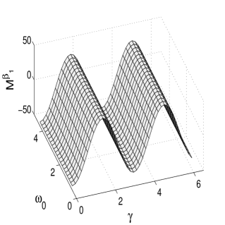
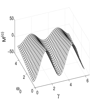
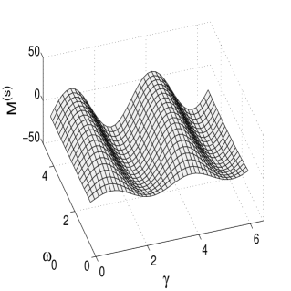
Figure 7. (a). The graph of $M^{(\beta_{1})}$ as a function of $\gamma$, and $M^{(\beta_{1})}$ is independent of $\omega_{0}$. (b). The graph of $M^{(c)}$ as a function of $\gamma$ and $\omega_{0}$. (c). The graph of the imaginary part of $M^{(s)}$ as a function of $\gamma$ and $\omega_{0}$.

Direct calculation gives that

$$M^{(a)}(\gamma)=M^{(0)}(\gamma)=M^{(b)}(\gamma)=0,\quad M^{(\alpha)}(\gamma)=91.3343,$$

and $M^{(\beta_{1})}$ and $M^{(c)}$ are real, while $M^{(s)}$ is imaginary. The graph of $M^{(\beta_{1})}$ is shown in Figure 7(a) (Notice that $M^{(\beta_{1})}$ is independent of $\omega_{0}$). The graph of $M^{(c)}$ is shown in Figure 7(b). The imaginary part of $M^{(s)}$ is shown in Figure 7(c).

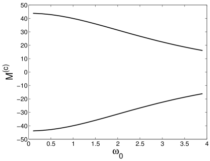
Figure 8. The graphs of $M^{(c)}$ along the curves (4.6).

In the case of only DC current ($\beta_{2}=0$), $M=0$ (4.2) leads to

(4.5) $$\alpha=-\beta_{1}M^{(\beta_{1})}/91.3343,$$

where $M^{(\beta_{1})}(\gamma)$ is a function of the internal parameter $\gamma$ as shown in Figure 7(a). In the general case ($\beta_{2}\neq 0$), $M^{(s)}(\gamma,\omega_{0})=0$ determines curves

(4.6) $$\gamma=\gamma(\omega_{0})=0,\ \pi/2,\ \pi,\ 3\pi/2,$$

and $M=0$ (4.2) leads to

(4.7) $$|\beta_{2}|>\bigg{|}\left(91.3343\alpha+\beta_{1}M^{(\beta_{1})}\right)\bigg{/}M^{(c)}\bigg{|},$$

where $M^{(\beta_{1})}$ and $M^{(c)}$ are evaluated along the curve (4.6), $M^{(\beta_{1})}=\pm 43.858$ (‘$+$’ for $\gamma=\pi/2,\ 3\pi/2$; ‘$-$’ for $\gamma=0,\ \pi$), $M^{(c)}$ is plotted in Figure 8 (upper curve corresponds to $\gamma=\pi/2,\ 3\pi/2$; lower curve corresponds to $\gamma=0,\ \pi$), and

$$\cos\left(\frac{\sigma\omega_{0}}{\sqrt{3}}\right)=-\frac{91.3343\alpha+\beta_{1}M^{(\beta_{1})}}{\beta_{2}M^{(c)}}.$$

5. Numerical Simulation

In the entire article, we use the finite difference method to numerically simulate the LLG (2.1). Due to an integrable discretization [9] of the Heisenberg equation (3.1), the finite difference performs much better than Galerkin Fourier mode truncations. As in (3.30), let $m(j)=m(t,jh)$, $j=1,\cdots,N$, $Nh=2\pi$, and $h$ is the spatial mesh size. Without further notice, we always choose $N=128$ (which provides enough precision). The only tricky part in the finite difference discretization of (2.1) is the second derivative term in $H$, for the rest terms, just evaluate $m$ at $m(j)$:

$$\partial_{x}^{2}m(j)=\frac{2}{h^{2}}\left(\frac{m(j+1)}{1+m(j)\cdot m(j+1)}+\frac{m(j-1)}{1+m(j-1)\cdot m(j)}\right).$$

5.1. Only DC Current Case

In this case, $\beta_{2}=0$ in (2.1), and we choose $\beta_{1}$ as the bifurcation parameter, and the rest parameters as:

(5.1) $$a=0.05,b=0.025,\alpha=0.02,\epsilon=0.01.$$

The computation is first run for the time interval [$0,8120\pi$], then the figures are plotted starting from $t=8120\pi$. The bifurcation diagram for the attractors, and the typical spatial profiles on the attractors are shown in Figure 9.

Figure 9. The bifurcation diagram for the attractors and typical spatial profiles on the attractors in the case of only DC current where $\beta_{1}$ is the bifurcation parameter, $c_{1}\cdots c_{6}$ are the bifurcation thresholds, and $c_{1}\in[0,0.01]$, $c_{2}\in[0.0205,0.021]$, $c_{3}\in[0.0231,0.0232]$, $c_{4}\in[0.025,0.026]$, $c_{5}\in[0.08,0.1]$, $c_{6}\in[0.13,0.15]$.

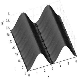
(a) $\beta_{1}=0.0205$ spatially non-uniform fixed point

(b) $\beta_{1}=0.023$ spatially non-uniform and temporally periodic or quasiperiodic attractor

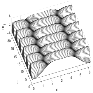
(c) $\beta_{1}=0.0235$ weak chaotic attractor

Figure 10. The spatio-temporal profiles of solutions in the attractors in the case of only DC current.

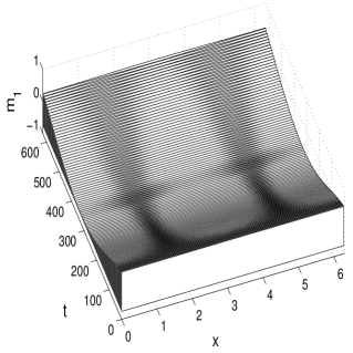
(a) $\beta_{1}=0.026$ spatially non-uniform and temporally periodic attractor

(b) $\beta_{1}=0.1$ spatially uniform and temporally periodic attractor

Figure 11. The spatio-temporal profiles of solutions in the attractors in the case of only DC current (continued).

This figure indiactes that interesting bifurcations happen over the interval $\beta_{1}\in[0,0.15]$ which is the physically important regime where $\beta_{1}$ is comparable with values of other parameters. There are six bifurcation thresholds $c_{1}\cdots c_{6}$ (Fig. 9). When $\beta_{1}<c_{1}$, the attractor is the spatially uniform fixed point $m_{1}=1$ ($m_{2}=m_{3}=0$). When $c_{1}\leq\beta_{1}\leq c_{2}$, the attractor is a spatially non-uniform fixed point as shown in Figure 10(a). When $c_{2}<\beta_{1}<c_{3}$, the attractor is spatially non-uniform and temporally periodic (a limit cycle) or quasiperiodic (a limit torus) as shown in Figure 10(b). Here as the value of $\beta_{1}$ is increased, first there is one basic temporal frequence, then more frequencies enter and the temporal oscillation amplitude becomes bigger and bigger. When $c_{3}\leq\beta_{1}<c_{4}$, the attractor is chaotic, i.e. a strange attractor as shown in Figure 10(c). Even though the chaotic nature is not very apparent in Figure 10(c), due to the smallness of the perturbation parameter together with smallness of all other parameters, the temporal evolution is chaotic, and we have used Liapunov exponent and power spectrum devices to verify this. When $c_{4}\leq\beta_{1}<c_{5}$, the attractor is spatially non-uniform and temporally periodic (a limit cycle) as shown in Figure 11(a). The spatial modulation is small, and it is even not apparent in Figure 11(a). But it is apparent on the individual typical spatial profiles as seen in region V in Figure 9. With the increase of $\beta_{1}$, the spatial modulation becomes smaller and smaller. When $c_{5}\leq\beta_{1}<c_{6}$, the attractor is spatially uniform and temporally periodic (a limit cycle, the so-called procession) as shown in Figure 11(b). When $\beta_{1}\geq c_{6}$, the attractor is the spatially uniform fixed point $m_{1}=-1$ ($m_{2}=m_{3}=0$).

When $\beta_{2}=0$, the Melnikov function predicts that around $\beta_{1}=0.041$ (4.5), there is probably chaos; while the numerical calculation shows that there is an interval [$0.0231,0.026$] for $\beta_{1}$ where chaos is the attractor. Since the perturbation parameter $\epsilon=0.01$ in the numerical calculation, the Melnikov function prediction seems in agreement with the numerical calculation.

Some of the attractors in Figure 9 are attractors of the corresponding ordinary differential equations by setting $\partial_{x}=0$ in (2.1), i.e. the single domain case. These attractors are the ones in regions I, VI and VII in Figure 9 [25] [41]. Because we are studying the only DC current case, the ordinary differential equations do not have any chaotic attractor [25] [41].

On the other hand, the partial differential equations (2.1) does have a chaotic attractor (region IV in Figure 9).

In general, when $\beta_{1}<0$, the Gilbert damping dominates the spin torque driven by DC current and $m_{1}=1$ is the attractor. When $\beta_{1}>0.15$, the spin torque driven by DC current dominates the Gilbert damping, $m_{1}=-1$ is the attractor, and we have a magnetization reversal. In some technological applications, $\beta_{1}>0.15$ may correspond too high DC current that can burn the device. On the other hand, in the technologically advantageous interval $\beta_{1}\in[0,0.15]$, magnetization reversal may be hard to achieve due to the sophisticated bifurcations in Figure 9.

5.2. Only AC Current Case

In this case, $\beta_{1}=0$ in (2.1), and we choose $\beta_{2}$ as the bifurcation parameter, and the rest parameters as:

(5.2) $$a=0.05,b=0.025,\alpha=0.0015,\epsilon=0.01,\omega_{0}=0.2.$$

Unlike the DC case, here the figures are plotted starting from $t=0$. It turns out that the types of attractors in the AC case are simpler than those of the DC case. When $\beta_{2}=0$, the attractor is a spatially non-uniform fixed point as shown in Figure 12. In this case, the only perturbation is the Gilbert damping which damps the evolution to such a fixed point. When $0<\beta_{2}<\beta_{2}^{*}$ where $\beta_{2}^{*}\in[0.18,0.19]$, the attractor is a spatially non-uniform and temporally periodic solution. When $\beta_{2}\geq\beta_{2}^{*}$, the attractor is chaotic as shown in Figure 12.

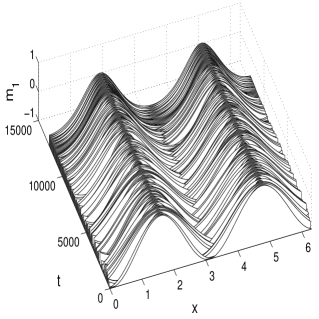
(a) $\beta_{2}=0$ spatially non-uniform fixed point

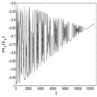
(b) $\beta_{2}=0$ temporal evolution at one spatial location

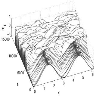
(c) $\beta_{2}=0.21$ chaotic attractor

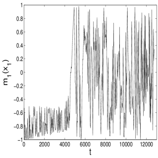
(d) $\beta_{2}=0.21$ temporal evolution at one spatial location

Figure 12. The attractors in the case of only AC current.

Figure 13. Homotopy deformation of the attractors under different initial conditions. See http://www.math.missouri.edu/~cli

Figure 14. The attractor when $\alpha=0.02$, $\beta_{2}=0.21$ and all other parameters’ values are the same with Figure 12. See http://www.math.missouri.edu/~cli

Our Melnikov prediction (4.7) predicts that when $|\beta_{2}|>0.003$, certain center-unstable and center-stable manifolds intersect. Our numerics shows that such an intersection seems leading to transient chaos. Only when $|\beta_{2}|>\beta_{2}^{*}$, the chaos can be sustained as an attractor. It seems that such sustained chaotic attractor gains extra support from parametric resonance due to the AC current driving [22], as can be seen from the turbulent spatial structure of the chaotic attractor (Fig. 12), which diverges quite far away from the initial condition. Another factor that may be relevant is the fact that higher-frequency spatially oscillating domain walls have more and stronger linearly unstable modes (3.5). By properly choosing initial conditions, one can find the homotopy deformation from the ODE limit cycle (procession) [25] [41] to the current PDE chaos as shown in Figure 13 at the same parameter values.

We also simulated the case of normal Gilbert damping $\alpha=0.02$. For all values of $\beta_{2}\in[0.01,0.3]$, the attractor is always non-chaotic. That is, the only attractor we can find is a spatially uniform limit cycle with small temporal oscillation as shown in Figure 14.

Of course, when neither $\beta_{1}$ nor $\beta_{2}$ is zero, the bifurcation diagram is a combination of the DC only and AC only diagrams.

6. Appendix: The Connection Between the Heisenberg Equation and the NLS Equation

In this appendix, we will show the details on the connection between the 1D cubic focusing nonlinear Schrödinger (NLS) equation and the Heisenberg equation (3.1). The nonlinear Schrödinger (NLS) equation

(6.1) $$iq_{t}+q_{xx}+2|q|^{2}q=0\ ,$$

is a well-known integrable system with the Lax pair

(6.2) $$\partial_{x}\phi = (i\lambda\sigma_{3}+U)\phi\ ,$$

(6.3) $$\partial_{t}\phi = -(2i\lambda^{2}\sigma_{3}+2\lambda U+V)\phi\ ,$$

where $\lambda$ is the complex spectral parameter, $\sigma_{3}$ is defined in (2.5), and

$$U=\left(\begin{array}[]{lr}0&iq\cr i\bar{q}&0\cr\end{array}\right)\ ,\quad V=-i|q|^{2}\sigma_{3}+\left(\begin{array}[]{lr}0&q_{x}\cr-\bar{q}_{x}&0\cr\end{array}\right)\ .$$

Lemma 6.1.

If $\phi=(\phi_{1},\phi_{2})^{T}$ solves the Lax pair (6.2)-(6.3) at $\lambda$, then $(-\overline{\phi_{2}},\overline{\phi_{1}})^{T}$ solves the Lax pair (6.2)-(6.3) at $\bar{\lambda}$. When $q$ is even, i.e. $q(-x)=q(x)$, then $(\overline{\phi_{2}}(-x),\overline{\phi_{1}}(-x))^{T}$ solves the Lax pair (6.2)-(6.3) at $-\bar{\lambda}$. When $\lambda$ is real, and $\phi$ is a nonzero solution, then $(-\overline{\phi_{2}},\overline{\phi_{1}})^{T}$ is another linearly independent solution. For any two solutions of the Lax pair, their Wronskian is independent of $x$ and $t$.

For any real $\lambda_{0}$, by the well-known Floquet theorem [28] and Lemma 6.1, there are always two linearly independent Floquet (or Bloch) eigenfunctions $\phi^{\pm}$ to the Lax pair (6.2)-(6.3) at $\lambda=\lambda_{0}$, such that

$$\phi^{+}=\left(\begin{array}[]{c}\varphi_{1}\cr\varphi_{2}\cr\end{array}\right)\ ,\quad\phi^{-}=\left(\begin{array}[]{c}-\overline{\varphi_{2}}\cr\overline{\varphi_{1}}\cr\end{array}\right)\ ,$$

$$\phi^{+}(x+2\pi)=\rho\phi^{+}(x)\ ,\quad\phi^{-}(x+2\pi)=\bar{\rho}\phi^{-}(x)\ ,\quad|\rho|^{2}=1\ .$$

Since the Wronskian $W(\phi^{+},\phi^{-})$ is independent of $x$ and $t$, without loss of generality, we choose $W(\phi^{+},\phi^{-})=1$. Then

$$S=\left(\begin{array}[]{lr}\varphi_{1}&-\overline{\varphi_{2}}\cr\varphi_{2}&\overline{\varphi_{1}}\cr\end{array}\right)$$

is a unitary solution to the Lax pair at $\lambda=\lambda_{0}$:

$$S^{-1}=S^{H}=\left(\begin{array}[]{lr}\overline{\varphi_{1}}&\overline{\varphi_{2}}\cr-\varphi_{2}&\varphi_{1}\cr\end{array}\right)\ ,\quad|\varphi_{1}|^{2}+|\varphi_{2}|^{2}=1\ .$$

Recall the definition of $\Gamma$ (2.7), let

$$\Gamma=S^{-1}\sigma_{3}S=\left(\begin{array}[]{lr}|\varphi_{1}|^{2}-|\varphi_{2}|^{2}&-2\overline{\varphi_{1}}\overline{\varphi_{2}}\cr-2\varphi_{1}\varphi_{2}&|\varphi_{2}|^{2}-|\varphi_{1}|^{2}\cr\end{array}\right)\ ,$$

i.e.

$$m_{1}+im_{2}=-2\varphi_{1}\varphi_{2}\ ,\quad m_{3}=|\varphi_{1}|^{2}-|\varphi_{2}|^{2}\ .$$

Now for any $\phi$ solving the Lax pair (6.2)-(6.3) at $\lambda$, define $\psi$ as

$$\psi=S^{-1}\phi\ .$$

Then $\psi$ solves the pair

(6.4) $$\psi_{x} = i(\lambda-\lambda_{0})\Gamma\psi\ ,$$

(6.5) $$\psi_{t} = -\left\{2i(\lambda^{2}-\lambda_{0}^{2})\Gamma+\frac{1}{2}(\lambda-\lambda_{0})[\Gamma,\Gamma_{x}]\right\}\psi\ .$$

The compatibility condition of this pair leads to the equation

(6.6) $$\Gamma_{t}=-\left\{4\lambda_{0}\Gamma_{x}+\frac{1}{2i}[\Gamma,\Gamma_{xx}]\right\}\ .$$

Setting $\lambda_{0}=0$ or performing the translation $t=t,\hat{x}=x-4\lambda_{0}t$, equation (6.6) reduces to the Heisenberg equation (3.2). Therefore, the Gauge transform $S$ transforms NLS equation into the Heisenberg equation. Periodicity in $x$ may not persist.

Example 6.2.

Consider the temporally periodic solution of the NLS equation (6.1),

$$q=ae^{i\theta(t)}\ ,\quad\theta(t)=2a^{2}t+\gamma\ .$$

The corresponding Bloch eigenfunction of the Lax pair (6.2)-(6.3) at $\lambda=0$ is

$$\varphi=\frac{1}{\sqrt{2}}\left(\begin{array}[]{c}e^{i\theta/2}\cr e^{-i\theta/2}\cr\end{array}\right)e^{iax}\ .$$

Then

$$\Gamma=S^{-1}\sigma_{3}S=\left(\begin{array}[]{lr}0&-e^{-i2ax}\cr-e^{i2ax}&0\cr\end{array}\right)\ ,$$

which is called a domain wall.

Acknowledgment: The second author Y. Charles Li is grateful to Professor Shufeng Zhang, Drs. Zhanjie Li and Zhaoyang Yang, and Mr. Jiexuan He for many helpful discussions.

References

- [1] L. Berger. Emission of Spin Waves by a Magnetic Multilayer. Phys. Rev. B, 54:9353–9358, 1996.
- [2] A. Calini. A Note on a Bäcklund Transformation for the Continuous Heisenberg Model. Phys. Lett. A, 203: 333–344, 1995.
- [3] M. Covington et al. Current-Induced Magnetization Dynamics in Current Perpendicular to the Plane Spin Valves. Phy. Rev. B, 69:184406, 2004.
- [4] A. Fabian et al. Current-Induced Two-Level Fluctuations in Pseudo-Spin-Valve (Co/Cu/Co) Nanostructures. Phys. Rev. Lett., 91:257209, 2004.
- [5] L. D. Faddeev, L. A. Takhtajan. Hamiltonian Methods in the Theory of Solitons. Springer-Verlag, Berlin, 1987.
- [6] G. D. Fuchs et al. Spin-Transfer Effects in Nanoscale Magnetic Tunnel Junctions. Appl. Phys. Lett., 85:1205, 2004.
- [7] J. Grollier, et al. Synchronization of Spin-Transfer Oscillators Driven by Stimulated Microwave Currents. arXiv:cond-mat/0509326, 2005.
- [8] Y. Ji et al. Current-Induced Spin-Wave Excitations in a Single Ferromagnetic Layer. Phys. Rev. Lett., 90:106601, 2003.
- [9] M. Kaashoek, A. Sakhnovich. Discrete Skew Selfadjoint Canonical Systems and the Isotropic Heisenberg Magnet Model. J. Funct. Anal., 228: 207-233, 2005.
- [10] S. Kaka, et al. Mutual Phase-Locking of Microwave Spin Torque Nano-Oscillators. Nature, 437: 389–392, 2005.
- [11] S. I. Kiselev et al. Microwave Oscillations of a Nanomagnet Driven by a Spin-Polarized Current. Nature, 425:380–383, 2003.
- [12] R. H. Koch et al. Time-Resolved Reversal of Spin-Transfer Switching in a Nanomagnet. Phys. Rev. Lett., 92:088302, 2004.
- [13] I. Krivorotov, et al. Time-Domain Measurements of Nanomagnet Dynamics Driven by Spin-Transfer Torques. Science, 307: 228–231, 2005.
- [14] K. Kudo, et al., Synchronized Magnetization Oscillations in F/N/F Nanopillars, arXiv:cond-mat/0511095, 2005.
- [15] Y. Li. Smale Horseshoes and Symbolic Dynamics in Perturbed Nonlinear Schrödinger Equations. Journal of Nonlinear Sciences, 9, no.4:363–415, 1999.
- [16] Y. Li. Chaos and Shadowing Around a Homoclinic Tube. Abstract and Applied Analysis, 2003, no.16:923–931, 2003.
- [17] Y. Li. Chaos and Shadowing Lemma for Autonomous Systems of Infinite Dimensions. J. Dynamics and Differential Equations, 15, no.4:699–730, 2003.
- [18] Y. Li. Homoclinic Tubes and Chaos in Perturbed Sine-Gordon Equation. Chaos, Solitons and Fractals, 20, no.4:791–798, 2004.
- [19] Y. Li. Chaos in Partial Differential Equations. International Press, 2004.
- [20] Y. Li. Persistent Homoclinic Orbits for Nonlinear Schrödinger Equation Under Singular Perturbation. Dynamics of PDE, vol.1, no.1, 87-123, 2004.
- [21] Y. Li. Existence of Chaos for Nonlinear Schrödinger Equation Under Singular Perturbation. Dynamics of PDE, vol.1, no.2, 225-237, 2004.
- [22] Y. Li. Chaos and Shadowing Around a Heteroclinically Tubular Cycle With an Application to Sine-Gordon Equation. Studies in Applied Mathematics, vol.116, 145-171, 2006, pp.165.
- [23] Y. Li and D. W. McLaughlin. Morse and Melnikov Functions for NLS Pdes. Comm. Math. Phys., 162:175–214, 1994.
- [24] Y. Li et al. Persistent Homoclinic Orbits for a Perturbed Nonlinear Schrödinger equation. Comm. Pure Appl. Math., XLIX:1175–1255, 1996.
- [25] Z. Li, Y. Li, S. Zhang. Synchronization, Modification and Chaos Induced by Spin-polarized Currents. Phys. Rev. B., 74:054417, 2006.
- [26] Z. Li and S. Zhang. Magnetization Dynamics with a Spin-Transfer Torque. Phys. Rev. B, 68:024404, 2003.
- [27] Z. Li and S. Zhang. Thermally Assisted Magnetization Reversal in the Presence of a Spin-Transfer Torque. Phys. Rev. B, 69:134416, 2004.
- [28] W. Magnus, S. Winkler. Hill’s Equation. Dover, NY, 1979.
- [29] J. Miltat et al. Spin Transfer into an Inhomogeneous Magnetization Distribution. J. Appl. Phys., 89:6982, 2001.
- [30] B. Mityagin. Spectral Expansions of One-Dimensional Periodic Dirac Operators. Dynamics of PDE, 1, no.2:125, 2004.
- [31] E. B. Myers et al. Current-Driven Switching of Domains in Magnetic Multilayer Devices. Science, 285:867–870, 1999.
- [32] B. Ozyilmaz et al. Current-Induced Magnetization Reversal in High Magnetic Fields in Co/Cu/Co Nanopillars. Phys. Rev. Lett., 93:067203, 2003.
- [33] M. R. Pufall et al. Materials Dependence of the Spin-Momentum Transfer Efficiency and Critical Current in Ferromagnetic Metal/Cu Multilayers. Appl. Phys. Lett., 83:323, 2003.
- [34] A. Slavin, et al. Nonlinear Self-Phase-Locking Effect in an Array of Current-Driven Magnetic Nanocontact. Phys. Rev. B, 72: 092407, 2005.
- [35] J. C. Slonczewski. Current-Driven Excitation of Magnetic Multilayers. J. Magn. Magn. Mater, 159:L1–L7, 1996.
- [36] J. Z. Sun. Current-Driven Magnetic Switching in Manganite Trilayer Junctions. J. Mag. Mag. Mater., 202:157, 1999.
- [37] S. Urazhdin et al. Current-Driven Magnetic Excitations in Permalloy-Based Multilayer Nanopillars. Phys. Rev. Lett., 91:146803, 2003.
- [38] J. E. Wegrowe. Magnetization Reversal and Two-Level Fluctuations by Spin Injection in a Ferromagnetic Metallic Layer. Phy. Rev. B, 68:2144xx, 2003.
- [39] S. A. Wolf et al. Spintronics: a Spin-Based Electronics Vision for the Future. Science, 294:1488, 2001.
- [40] M. Yamanouchi et al. Current-Induced Domain-Wall Switching in a Ferromagnetic Semiconductor Structure. Nature, 428:539, 2004.
- [41] Z. Yang, S. Zhang, Y. Li. Chaotic Dynamics of Spin Valve Oscillators. Phys. Rev. Lett., 99: 134101, 2007.
- [42] J. G. Zhu et al. Spin Transfer Induced Noise in CPP Read Heads. IEEE Trans. on Magn., 40:182, 2004.