Unjamming due to local perturbations in granular packings with and without gravity

Abstract

We investigate the unjamming response of disordered packings of frictional hard disks with the help of computer simulations. First, we generate jammed configurations of the disks and then force them to move again by local perturbations. We study the spatial distribution of the stress and displacement response and find long range effects of the perturbation in both cases. We record the penetration depth of the displacements and the critical force that is needed to make the system yield. These quantities are tested in two types of systems: in ideal homogeneous packings in zero gravity and in packings settled under gravity. The penetration depth and the critical force are sensitive to the interparticle friction coefficient. Qualitatively, the same nonmonotonic friction dependence is found both with and without gravity, however the location of the extrema are at different friction values. We discuss the role of the connectivity of the contact network and of the pressure gradient in the unjamming response.

I Introduction

Many systems including granular materials, foams and emulsions can flow like fluids when a high external stress is applied but jam into a solidlike state below a certain threshold of stress. In a jammed state Liu and Nagel (1998, 2001); Makse et al. (2004); Kolb et al. (2004) the many-body system is trapped in a metastable configuration far from equilibrium where the constituent particles block each others motion. For a typical jammed granular packing, where the thermal fluctuations are negligible, only a sufficiently high external stress can lead to an unjamming transition and cause rearrangements of the particles.

In this paper we study the unjamming response of dense disordered granular media based on computer simulations. To achieve the unjamming transition we perturb the material by generating a small local deformation. These perturbations break the static structure of the packings and induce motion of particles.

The response of granular media to local perturbations have been studied widely both in experiments Geng et al. (2001); Kolb et al. (2004); Serero et al. (2001); Kolb et al. (2006); Atman et al. (2005) and in computer simulations Atman et al. (2005); Goldenberg and Goldhirsch (2005); Ostojic and Panja (2006); Goldenberg et al. (2006). The majority of these studies apply small force overloads to study the stress response inside the bulk of material. In these cases, the displacements originate only from elastic deformation of the particles; the system remains in the jammed state. Unjamming induced by local perturbation has been also investigated experimentally. Kolb and co-workers Kolb et al. (2004, 2006) studied two-dimensional packings of disks under gravity and applied localized cyclic perturbations to achieve real plastic rearrangements. Based on the displacement field they showed that the unjamming response is long ranged; the magnitude of the particle displacements decays as a power law of the distance from the perturbation source. The exponent of the decay varied between $0.6$ and $1.4$ depending on the preparation of the system.

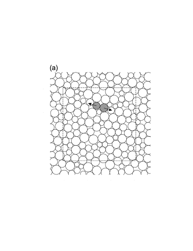
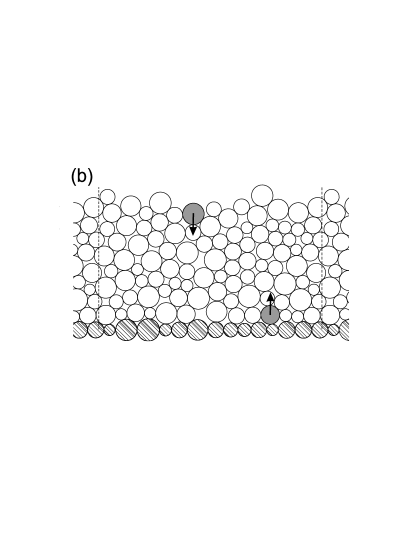
Figure 1: Schematic picture of the two types of granular packings confined by an external pressure bath (a) and by gravity (b). The dashed lines mark periodic boundaries. Some typical perturbations are illustrated with gray particles and arrows showing the direction of perturbation.

Here we focus on the question of what role the interparticle friction and gravity play in the unjamming transition. We study the unjamming response with the help of the contact dynamics method Moreau (1994); Jean (1999); Brendel et al. (2004) which handles the particles as perfectly rigid bodies. Therefore elastic distortion of the particles are excluded and the generated particle movements correspond to real plastic rearrangements. We analyze the response of the packing to local perturbations by considering the individual particle displacements, the coarse-grained displacement field, and, in addition, the resistance of the system against the deformation. We show that the stability of the packing against local perturbations depends strongly and in a nontrivial way on the particle-particle friction coefficient. Our systems are two-dimensional disordered packings of disks. First, we test ideal homogeneous packings prepared by an isotropic external pressure and with fully periodic boundary conditions Shaebani et al. (2007); Shaebani et al. (2008a) [Fig. 1(a)]. This part is the full exposition and expansion of the results presented and considered from another point of view in Shaebani et al. (2007). Then we study more realistic packings that are settled under gravity [Fig. 1(b)]. The packings are perturbed by moving two adjacent particles apart in the former case and by shifting one particle vertically in the latter case.

This work is organized in the following manner: Section II contains the description of the simulation method. In Sec. III we present our results for the perturbation of homogeneous packings. The perturbation of the packings that are settled under gravity is investigated in Sec. IV. The role of the different preparation and perturbation methods are discussed in Sec. V. Finally Sec. VI concludes the paper.

II simulation method

We perform contact dynamics simulations on 2D granular packings of cohesionless perfectly rigid disks. The numerical results of the local perturbations are presented for two distinct settings: (i) homogeneous random packings confined by an external pressure in the absence of gravity [Fig. 1(a)] and (ii) packings confined by gravity [Fig. 1(b)]. In both cases, the numerical experiments consist of two steps. First we prepare static configurations of grains; then, we probe the packings by perturbing their local structure. We apply the contact dynamics method Jean (1999); Brendel et al. (2004) for both procedures. The details of the numerical methods are described for homogeneous and inhomogeneous settings in Secs. II.1 and II.2, respectively.

In the rest of the paper we have the following conventions. The unit of the length is set to the maximum grain radius. As we examine 2D systems, the disks have polydispersity to avoid crystallization characteristic for two-dimensional monodisperse ensembles. We use a uniform distribution of the disk radii over the range between 0.5 and 1. The unit of the mass is set by assuming that the material of the grains has unit density and the masses of the disks are proportional to their areas.

II.1 Homogeneous random packings

We first examine the homogeneous configurations of disks. Here, the acceleration of gravity is set to zero in order to avoid force gradients in the samples. The number of the grains contained by the packings ranges from $500$ to $8000$. As mentioned above, we first generate static dense random packings by compressing the initial configuration of the particles into a smaller space. The compaction starts with a square box filled with loose granular gas. The disks are initially placed at random without overlaps. We apply periodic boundary conditions to avoid wall effects. In order to achieve homogeneous packings, we generalized the method proposed by Andersen Andersen (1980) to contact dynamics (for details see Shaebani et al. (2008a)). The main idea in this method is that, instead of using pistons, compaction is achieved by imposing a constant external pressure $P_{\text{ext}}$ and let the volume of the cell evolve in time. In fact, the volume of the system, which acts as an additional degree of freedom, couples with a confining pressure bath, so that the volume change is controlled by the difference between the external and internal pressures.

As the size of the cell shrinks due to the difference between $P_{\text{ext}}$ and the internal pressure $P_{\text{in}}$, at some point the grains cannot avoid touching each other anymore, and start building up an inner pressure to avoid interpenetration. Finally all motion stops because the grains block further compaction. The sample is considered to have converged to mechanical equilibrium when further time evolution leads to negligible changes in the particle positions. At this point we have a static jammed configuration under external pressure. The mechanical equilibrium is achieved for each grain and the corresponding $P_{\text{in}}$ equals $P_{\text{ext}}$. It is worth noting that the packing configurations depend on the friction coefficient $\mu$. We construct a new packing for each value of $\mu$ before starting the perturbation process.

The perturbation is carried out in the following way: We choose two adjacent particles in contact and force them to move apart [Fig. 1(a)]. As this case has been described in Shaebani et al. (2007), here only a short review is given. At the perturbation point we enforce the contacting surfaces to open up to a small gap and determine the force that is needed to fulfill this constraint (critical force). This concept is suited very well to the contact dynamics method where interparticle forces are handled as constraint forces, i.e., they are calculated based on constraint conditions which prescribe the relative motion of the contact surfaces Jean (1999); Brendel et al. (2004). With enforcing the opening of the contact, we bring the system immediately to the yield point where the perturbation induces sliding and/or opening of some contacts and initiates collective rearrangements of the particles at least in the vicinity of the perturbation point. It is beneficial to choose small gap size as we are interested in the onset of motion, how the static structure breaks due to the perturbation. Large deformations, e.g., creation of new contacts, are out of the scope of the present study. We checked that for small gap sizes the displacement field (up to a constant factor) and the critical force become independent of the size of the gap. Our numerical measurements are performed in this gap-independent region; the size of the gap $\xi$ is set to $10^{-9}$ Shaebani et al. (2007). This value is far larger than the displacement scale $10^{-14}$ that arises from the noise level of particle velocities.

The perturbation process can be performed under two different boundary conditions. One can either impose the fixed external pressure condition in continuation of the assembling process, or impose the fixed volume condition. In the former method, the pressure of the system is constant and the volume is allowed to change during the perturbation while in the latter method, the volume is fixed and the pressure changes due to perturbation. This paper mainly contains the results of perturbation method with fixed pressure even though we compare some numerical results of both methods in Sec. III.3 and find no significant differences.

II.2 Packings confined by gravity

In the inhomogeneous case, the system is settled under gravity and no pressure bath is used. Consequently there exists a pressure gradient in the vertical direction. We present simulations on model systems of $N=1600$ polydisperse disks. The system is spatially periodic in the horizontal direction, and a one-dimensional chain of disks with random radii is fixed at the bottom of the box to provide a rough bed [see Fig. 1(b)]. The particle-particle and particle-base friction coefficients are the same. The starting configuration is a dilute granular medium which consists of randomly distributed nonoverlapping particles with zero velocities. The average initial packing fraction $\phi$ ranges from $0.32$ to $0.40$ for different packings. Next the system is allowed to settle on top of the rough bed under the influence of the gravitational acceleration $g$. We wait until the packing relaxes into equilibrium. The average static packing height ranges from $35.2\pm 0.1$ (approximately $23$ layers of grains) for samples with small friction coefficient $\mu=10^{-8}$ to $36.9\pm 0.1$ ($\sim 25$ layers) for samples with large friction coefficient $\mu=10$. This construction method mimics the pouring of grains through a sieve far away from lateral walls.

To investigate the effect of friction and also to measure the displacement response with better statistics, $20$ packings are constructed and perturbed for each value of the friction coefficient $\mu$.

After that we turn to the perturbation part where we perturb the topmost or lowermost particles in two different experiments in order to test the effect of local perturbation in the inhomogeneous system [Fig. 1(b)]. In the first case, we choose a particle at the free surface of the packing and force it to move vertically downwards by a small displacement $\xi$. We measure the generated displacements of the particle centers and also the force response of the system on the perturbed particle. This latter is the vertical component of the sum of the contact forces acting on the perturbed particle, which plays the role of the critical force.

In the case where the system is perturbed from the bottom we choose a particle at the lowermost part of the sample and force it to move vertically upwards by a small upwards shift $\xi$. The displacement pattern and the critical force are measured. In both cases, the magnitude of the displacement $\xi$ is set to the same value as the gap for the homogeneous system.

III Perturbation of homogeneous packings

In this section, we will analyze the mechanical response of the homogeneous packing to the local perturbation which we introduced in Sec. II.1 and see how the response changes with the friction coefficient. The results presented in this section belong to the system size $N=3000$ unless explicitly stated otherwise.

After opening up a contact that is selected for the perturbation, we study the generated displacement field of particle centers and the perturbation force which is needed to open up the contacting surfaces at the perturbation point. This critical force $F_{\text{crit}}$ characterizes the strength of the system against the local perturbation. Furthermore, the numerical results are compared for the fixed pressure and the fixed volume perturbation methods. We close this section by reporting the results of the generated force and stress response fields.

III.1 Displacement response field

Our aim here is to find out how far the rearrangements have to penetrate into the packing as a consequence of the prescribed local deformation. Is there a related length scale?

Our results reveal that the displacement of particle centers due to the single contact perturbation form a disordered vector field. This response field can be relatively localized [Fig. 2(a)] or more widespread [Fig. 2(b)] depending on the location of perturbation.

Figure 2: (a),(b) Displacement response fields in the laboratory frame for two different locations of the perturbation. The resulting vector field can be relatively localized (a) or more widespread (b) depending on the perturbed contact. (c) Displacement response field in the contact frame averaged over several thousand perturbations. The system contained $3000$ disks with friction coefficient $0.5$. The unit of the length, in which $x$ and $y$ are measured, is set to the maximum grain radius. For clarity, the magnitude of the displacements has been increased by a factor of $10^{11}$ in all figures.

As a measure for the magnitude of the displacement response, we define the penetration depth $\delta$ as

$$\delta=\frac{\displaystyle\sum_{\text{i=1}}^{\text{N}}|\vec{d}_{\text{i}}||\vec{r}_{\text{i}}\cdot\vec{n}|}{\displaystyle\sum_{\text{i=1}}^{\text{N}}|\vec{d}_{\text{i}}|},$$ (1)

where the sum runs over all particles, $\vec{d}_{\text{i}}$ is the displacement vector of the $i$th particle center, $\vec{r}_{\text{i}}$ is the distance vector from the perturbed contact to the $i$th particle center, and $\vec{n}$ is the unit contact normal of the perturbed contact.

The penetration depth $\delta$ characterizes the size of the rearrangement zone in the direction of the contact normal. $\delta$ exhibits large fluctuations depending on the perturbed contact. For the displacement fields shown in Figs. 2(a) and 2(b) the values of $\delta$ are $7.68$ and $23.31$, respectively. The average penetration depth $\langle\delta\rangle$, which we calculated based on the perturbation of $1500$ randomly chosen contacts of the same system, is $19.8\pm 0.1$.

Figure 3: The magnitude of the average displacements $d$ in terms of the distance from the perturbed contact $r$. Here $\xi$ stands for the gap generated at the perturbed contact. Different slopes correspond to different friction coefficients $\mu$. For each value of friction four systems of different sizes are investigated. The total number of particles is between $500$ and $8000$. The error bars remain below $5\%$ of the values $d(r)/\xi$ for the whole range of $r$.

In order to study the average properties of the displacement fields, we perturb all contacts one by one, always starting with the original static packing. In each case the particle movements are recorded in the local contact frame where the perturbed contact sits in the origin and the $x$ axis is chosen parallel to the contact normal, i.e., $x$ indicates the direction of the separation, then we calculate the average displacement field.

Figure 2(c) shows a smooth displacement field obtained by averaging over all perturbed contacts. The circular shape in Fig. 2(c) is achieved because the original square shape of the system has many different orientations when transformed into different contact frames. Similar quadrupolar structures as in Fig. 2(c) were found for shearing amorphous systems, where localized quadrupolar rearrangements appear at the onset of plastic events Maloney and Lemaitre (2006).

The magnitude of the average displacement vectors $d$ decays with the distance $r$ from the perturbation point as shown in Fig. 2(c). In order to investigate its decay, we calculate $d$ by averaging out the angle of the position. Figure 3 shows that the magnitude of rearrangements $d$ decays as a power law of the distance $r$,

$$d\propto r^{-\alpha}.$$ (2)

Different slopes in Fig. 3 correspond to different friction coefficients. However, the exponent $\alpha$ is approximately independent of the system size. This can be seen more clearly in Fig. 4(a), in which the exponent is shown in terms of the total number of particles $N$ for three different frictions. Our results show that $\alpha$ lies in the range $0.7-1.4$. The results of a recent experiment performed by moving an intruder in a system of disks Kolb et al. (2006) displays similar power-law behavior with the same range of $\alpha$.

The power-law decay of the average displacements indicates that there is no characteristic size for the rearrangement zone; instead, a decay exponent may be more suitable to characterize the particle movements. Therefore the rearrangement region is not bounded on sides by a penetration length and the quantity $\delta$ may not remain finite for an infinitely large system. Despite of these facts, $\delta$ is still a useful measure of the displacements for finite systems. Using $\delta$, one can still compare two displacement fields for the same system size. Larger $\delta$ means a larger rearrangement zone. Moreover, $\delta$ can be easily measured also for single perturbations where the usage of $\alpha$ would be troublesome. The exponent $\alpha$ works well for the average displacement field but it is not a well defined quantity for single perturbations where the fluctuation of $d(r)$ is so large that it cannot be fitted with a power-law decay.

To investigate the role of friction, we perturb several packings constructed already with different friction coefficients, $\mu$. The average penetration depth $\langle\delta\rangle$ has a strong dependence on the friction coefficient $\mu$. It is a nonmonotonic function with a sharp minimum at $\mu\approx 0.1$ [Fig. 5 (solid circles)]. Equivalent behavior is found for $-\alpha$ as a function of $\mu$ in Ref. Shaebani et al. (2007). When the friction is increased starting from zero, the decrease of $\langle\delta\rangle$ indicates that the induced rearrangements become more localized. At $\mu\approx 0.1$ the process takes a sharp turn and further increase of the friction leads to delocalization.

Figure 4: Dependence of the penetration exponent $\alpha$ (a) and the mean critical force $\langle F_{\text{crit}}\rangle$ (b) on the system size $N$ for three different friction coefficients $\mu$.

III.2 Critical force

We now turn our attention to the critical force $F_{\text{crit}}$. The results show that $F_{\text{crit}}$ depends also strongly on the place of the perturbation. First we check its average properties.

The average critical force $\langle F_{\text{crit}}\rangle$ again shows strong dependence on the friction coefficient [Fig. 5 (open circles)] and remains approximately constant under changing the system size [Fig. 4(b)]. Here, $\langle F_{\text{crit}}\rangle$ is scaled by the average normal contact force $\langle F_{\text{cont}}\rangle$. In $\langle F_{\text{cont}}\rangle$, only the normal component of the contact forces is taken into account and the average $\langle\cdot\cdot\cdot\rangle$ is taken over all the contacts of the given packing.

Figure 5: Average critical force $\langle F_{\text{crit}}\rangle$ (open circles) scaled by the average normal contact force $\langle F_{\text{cont}}\rangle$ and the average penetration depth $\langle\delta\rangle$ (full circles) as functions of the friction coefficient $\mu$. The vertical dashed line emphasizes that the two extrema are located at the same $\mu$.

Both the critical force and the penetration depth show the characteristic nonmonotonic behavior (Fig. 5) in contrast to other quantities that describe the properties of the packing. E.g., the average coordination number $z$, the average contact force $\langle F_{\text{cont}}\rangle$, and the packing fraction exhibit smooth and monotonic functions of the friction coefficient with plateaus for the low and high friction regions Shaebani et al. (2007). $F_{\text{crit}}$ and $\delta$ behave completely differently. They exhibit sharp extrema at the same friction: At $\mu\approx 0.1$ the maximum critical force and the most localized rearrangement zone is observed which has the meaning that the packing constructed with friction $\mu=0.1$ is the most stable packing against local perturbations. Moving towards the higher or lower friction coefficients, packings get weaker against the perturbation, the critical force becomes smaller, and the induced rearrangements become more widespread.

Figure 6: Each data point represents one contact in the frame of the critical force $F_{\text{crit}}$ and the normal component of the original contact force $F_{\text{cont}}$. The four figures correspond to four packings constructed with different frictions. $\langle F_{\text{cont}}\rangle$ is the average normal contact force in each packing. The dashed lines correspond to $F_{\text{crit}}=F_{\text{cont}}$.

Figure 7: Probability distribution of the critical forces $F_{\text{crit}}$ (a) and the critical forces normalized with respect to their mean in each packing $F_{\text{crit}}/\langle F_{\text{crit}}\rangle$ (b) for different friction coefficients. The inset displays a semilogarithmic plot of probability distribution of the normalized critical forces when averaged over all friction coefficients. The dashed line is an exponential fit of the tail of the curve.

To get more insight into the force response we examine $F_{\text{crit}}$ at every contact separately. Figure 6 reveals that the critical force is strongly correlated with the original contact force. For small values of $\mu$ a pair of contacting particles cannot resist a force of separation larger than the force itself that originally presses the two contact surfaces together. This can be understood well in the case of zero friction where the structure is isostatic Roux (2000), where the structure and the external load $p_{\text{ext}}$ determine uniquely what equilibrium force is acting between a selected pair of contacting particles. If one pushes the two particles apart with a larger force, it should be compensated by a negative contact force. As the contact cannot exert negative forces we lose one constraint and, consequently, one floppy mode Roux (2000) appears in the system allowing collective motion of the particles.

Naturally, the critical force never falls below the actual contact force, however, for the frictional case it can get larger. This can be best seen for $\mu=0.1$ in Fig. 6. For further increase of $\mu$ the picture becomes similar to the case of zero friction, i.e., the force response of a contact against opening is basically given by the normal component of the original contact force.

It is known that contact forces in random packings of frictional rigid grains are not determined uniquely by the mechanical equilibrium and Coulomb condition Snoeijer et al. (2004); Unger et al. (2005); McNamara et al. (2005); Ostojic and Panja (2006). There is an ensemble of admissible force networks that satisfy all of these conditions in the same configuration of grains. The extent of the force indeterminacy as a function of the friction coefficient $\mu$ was numerically examined in Unger et al. (2005) for packings of rigid disks, where a nonmonotonic friction dependence was found with a maximum value at $\mu\approx 0.1$. A direct connection between the critical force $F_{\text{crit}}$ and the extent of the indeterminacy at a given contact is established in Shaebani et al. (2007) where it was found that the critical force equals the maximum possible contact force at the same contact taken over the ensemble of admissible force networks. For further details on the consequence of force indeterminacy the reader is referred to Shaebani et al. (2007); Unger et al. (2005); Shaebani et al. (2008b).

Figure 8: The correlation between the critical force $F_{\text{crit}}$ (full circles) or the normal component of the original contact force $F_{\text{cont}}$ (open circles) and the penetration depth $\delta$ in terms of the friction coefficient $\mu$.

As we mentioned before, the value of the critical force widely changes depending on the perturbed contact. The probability distributions for $F_{\text{crit}}$ are displayed in Fig. 7(a) for different friction coefficients. The critical forces are scaled in units of $F_{\text{0}}$ set by the external pressure and by the average radius of the particles, $F_{\text{0}}=2R_{\text{avg}}P_{\text{ext}}$. Here, we use the unit $F_{\text{0}}$ because, unlike $\langle F_{\text{cont}}\rangle$, it provides a fixed force scale for all systems which is independent of the friction coefficient. Figure 7(a) shows that the probability distributions depend strongly on $\mu$. With increasing friction, probability distributions become broader and the curves are shifted. The shift is nonmonotonic as expected from the behavior of $\langle F_{\text{crit}}\rangle$. The curves move rightwards and then leftwards below and above $\mu=0.1$, respectively.

Figure 9: Comparison of the results of the fixed pressure (solid circles) and the fixed volume (open circles) perturbation methods. (a) The penetration depth $\delta$ and (b) the critical force $F_{\text{crit}}$ for several contacts subjected to the perturbation. (c) The relative change in the size of the system $\lambda$ (solid circles) and the pressure $P$ (open circles) obtained during the perturbation of each contact with the fixed pressure and fixed volume methods, respectively. Here, the friction coefficient is $0.5$.

When normalized with respect to their mean values, these distributions are approximately independent of the friction coefficient [Fig. 7(b)] and their tail can be fitted with an exponential decay

$$P(F_{\text{crit}}/\langle F_{\text{crit}}\rangle)\propto e^{(-\beta)F_{\text{crit}}/\langle F_{\text{crit}}\rangle}$$ (3)

where $\beta=2.3\pm 0.1$ when averaged over all friction coefficients [see the inset of Fig. 7(b)].

The tail of the curves in Fig. 7(b) for the critical forces is reminiscent of the tail of the probability distributions of the contact forces which has been studied extensively in the literature Mueth et al. (1998); Radjai et al. (1996); Goldenberg and Goldhirsch (2003); Majmudar and Behringer (2005); van Eerd et al. (2007). This similarity can be understood well, based on the strong correlation between the critical force and the original contact force which is described in Fig. 6.

Next we focus on the correlation between the critical force $F_{\text{crit}}$ and the penetration depth $\delta$. Figure 8 (solid circles) displays that there is a weak correlation between these two quantities with a maximum value again around $\mu=0.1$ and it vanishes for large friction coefficients. The existence of the correlation means that, on average, a slightly larger rearrangement zone is expected for a larger critical force. Open circles in Fig. 8 reveal smaller correlations between the normal component of the original contact force $F_{\text{cont}}$ and $\delta$.

III.3 Fixed pressure and fixed volume perturbations

In Sec. II.1 we mentioned that one can perturb the system by imposing either the fixed external pressure condition or the fixed volume condition. In this section we compare these two perturbation methods by applying them in the same test system on the same list of contacts. The penetration depth $\delta$ and the critical force $F_{\text{crit}}$ are shown for each perturbed contact in Figs. 9(a) and 9(b), respectively. The results of the two methods are very similar to each other even though the imposed boundary conditions are basically different.

In the fixed volume method the pressure $P$ is allowed to change, while in the fixed pressure method the variable quantity is the volume of the system. Let us measure the volume change by $\lambda=\Delta L/L$, where $L$ is the size of the system. Figure 9(c) shows that there is a strong correlation between the variable quantities $P$ for one method and $\lambda$ for the other. The expansion (contraction) of the system due to the perturbation of a contact with the fixed pressure method corresponds to pressure increase (decrease) when perturbing the same contact with the fixed volume method.

III.4 Force and stress response fields

Figure 10: The average magnitude of the change in the normal component of contact forces due to the perturbation $\langle|\Delta F|\rangle$ scaled by $F_{\text{0}}$ in terms of the distance from the perturbed contact $r$. Different curves correspond to different friction coefficients $\mu$.

Finally, we investigate how other contact forces and the corresponding stress field is changed by the local perturbation. We measure the average magnitude of the change in the normal component of the contact forces $\langle|\Delta F|\rangle$ which is caused by the perturbation. Figure 10 shows $\langle|\Delta F|\rangle$ as a function of the distance from the perturbed contact. These curves, unlike the displacement response, do not follow a power law decay. Close to the perturbation point, much larger $\langle|\Delta F|\rangle$ is observed for $\mu=0.1$ than for the extreme values of friction ($\mu=10^{\text{-8}}$, $10$). Depending on the friction, $\langle|\Delta F|\rangle$ can be changed even by a factor $30$ in the vicinity of the perturbation point. The values of $\langle|\Delta F|\rangle$ become closer to each other for different frictions far away from the perturbation point since the decay of $\langle|\Delta F|\rangle$ becomes steeper for intermediate values of friction. Apparently $|\Delta F|$ goes to zero with $r$ leading to tiny changes in the contact forces far away from the perturbation point. Interestingly, even these tiny forces are able to break the solid state of the packing and induce rearrangements of the particles (Fig. 2).

We calculate the average stress field caused by the perturbation, measured always in the contact frame and averaged over several thousands of perturbations. We divide the system into square grid boxes of size $2$. This corresponds to the maximum diameter or twice the minimum diameter of the particles. The whole stress we achieved for each box is assigned to the position of the center of the box. The stress tensor $\sigma_{\alpha\beta}$ in each grid box is given Christoffersen et al. (1981) by

$$\sigma_{\alpha\beta}=\frac{1}{V}\displaystyle\sum_{i<j}\theta_{\text{ij}}f^{\alpha}_{\text{ij}}r^{\beta}_{\text{ij}},$$ (4)

where $V$ is the area of the box, $f^{\alpha}_{\text{ij}}$ is the $\alpha$ component of the force exerted on particle $i$ by particle $j$, and the vector $\vec{r}_{\text{ij}}$ points from the center of particle $i$ to the center of $j$ (one has to take the periodic boundary conditions into account and involve nearest image neighbors). The sum runs over all pairs of contacting particles. $\theta_{\text{ij}}$ is a number between $0$ and $1$ that gives what fraction of the line segment connecting the centers of the two particles is located in the box. Thus if the line segment is cut by grid lines the stress contribution of the contact is divided among the corresponding boxes.

First we investigate the pressure which is defined as half of the trace of the stress tensor. Originally (before perturbation) the pressure is spatially constant due to the symmetry of the compression process. To investigate the effect of perturbation on the local pressure, we calculate the pressure change as

$$\Delta P=\frac{1}{2}\text{tr}(\sigma-\sigma_{\text{0}}),$$ (5)

where $\sigma_{\text{0}}$ is the stress tensor before the perturbation.

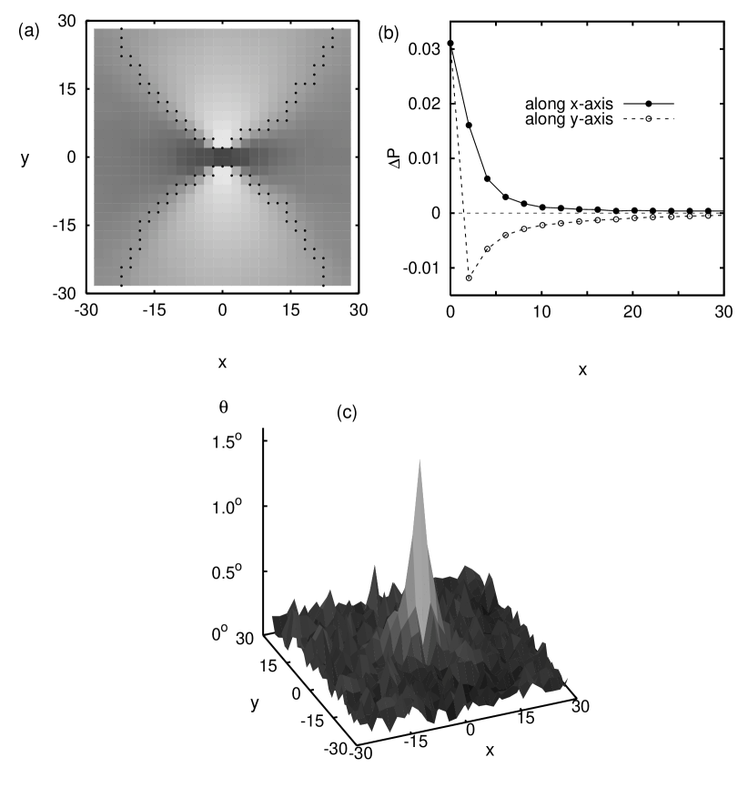
Figure 11: (a) The profile of the pressure change $\Delta P$. Shading is logarithmic in the amplitude of the pressure change, with black indicating a pressure increase, and white, a pressure decrease. Dots show where the sign of $\Delta P$ is changed. (b) $\Delta P$ along the $x$ and $y$ axes. (c) The maximum angle of friction mobilization $\alpha_{\text{max}}$. The $x$ axis indicates the direction of separation at the perturbed contact. The friction coefficient is $0.5$.

Figure 11(a) shows a logarithmic shading of the pressure change with black indicating a pressure increase, and white, a pressure decrease. This figure reveals that the pressure change decays fast with the distance from the perturbation point. The borders between the regions of positive and negative $\Delta P$ are also indicated in Fig. 11(a). $\Delta P$ is positive (negative) along (perpendicular to) the perturbation direction. For ease of comparison Fig. 11(b) shows $\Delta P$ along and perpendicular to the $x$ axis in the contact frame.

Next we investigate the angle of shearing, which is usually used to describe how close the material is to plastic deformation. The angle of shearing $\theta$ is provided by the local stress tensor Nedderman (1992):

$$\theta=\arcsin\left(\frac{\tau_{\text{max}}}{P}\right)=\arcsin\left(\frac{\sqrt{\sigma^{\text{2}}_{\text{xy}}+(\sigma_{\text{xx}}-P)^{\text{2}}}}{P}\right).$$ (6)

When the shear stress is measured in an imaginary plane at some point of the material, its value depends on the orientation of the plane. For a given stress state, $\tau_{\text{max}}$ denotes the maximum shear stress among all orientations. Dry granular media are often characterized by a critical angle of shearing resistance $\theta_{\text{crit}}$ Nedderman (1992). The material is expected to behave as solid until the angle of shearing remains below the critical angle and plastic deformation occurs when the critical angle is reached.

Since the local stress is symmetric before the perturbation, the initial value of the local angle of shearing $\theta_{\text{0}}$ is approximately zero. $\theta$ induced by the perturbation exhibits also a fast decay away from the perturbed contact. Figure 11(c) shows that $\theta$ is very small throughout the system. Interestingly, even the largest value $\theta\approx 1.5^{\circ}$ is far below the critical angle (the typical value of $\theta_{\text{crit}}$ is around $20^{\circ}-30^{\circ}$), still the perturbation is able to break the solid structure of the packing.

IV Perturbation of packings confined by gravity

In this section we present the numerical results of the local perturbations of packings confined by gravity. It it important to note that both preparation and perturbation steps are performed in the presence of gravity. In Sec. II.2 we explained how such static configurations are prepared. We also described how we perturb the topmost and lowermost particles in two different measurements. Actually, these systems are more realistic in the preparation and perturbation methods than those investigated in Sec. III.

Our main aim is to study whether the nonmonotonic friction dependence of the mechanical response found for the ideal homogeneous packings is reproduced in these realistic systems. Here, by shifting a particle downwards at the free surface or upwards at the bottom of the packing, we study the generated rearrangements of the particle centers and also the critical force on the perturbed particle.

We start our investigation with the results of the displacement response field. We find that particle movements are not bounded to a small vicinity of the perturbation point but we observe displacements even in regions of the system that are far from the perturbed particle. This indicates a long range effect similar to those found for homogeneous packings (Sec. III) and in experiments Kolb et al. (2004, 2006).

Here again, we characterize the size of the rearrangement zone in our finite systems with the penetration depth $\delta$. Similarly to Sec. III, $\delta$ is defined by the same expression [Eq. (1)] also in the present case, only $\vec{r}_{i}$ now denotes the distance vector from the center of the perturbed particle to the center of the $i$th particle and $\vec{n}$ is pointing vertically downwards (upwards) for top perturbations (bottom perturbations). Thus $\delta$ has the meaning of the vertical size of the rearrangement zone. Similar to the homogeneous case, $\delta$ depends strongly on the perturbed particle; therefore we repeat the perturbation for many particles to obtain the average value $\langle\delta\rangle$.

$\langle\delta\rangle$ is recorded separately for top and bottom perturbations and for each value of friction. In each case, the average value $\langle\delta\rangle$ is calculated over approximately $1000$ perturbed particles. These particles are selected as follows. We divide the width of the system into several bins of size roughly equal to the average diameter of the particles. Among the particle centers located at the same bin, we find the highest and lowest centers and the corresponding two particles are selected for the top and bottom perturbations, respectively. We repeat this procedure for each bin.

It has to be noted that not all the selected particles for bottom perturbation are taken into account in the calculation of $\langle\delta\rangle$. We exclude rattler particles that do not take part in the force transmission because they are screened by a local arch. Of course, there are no true rattlers in the presence of gravity, because every particle inevitably has force carrying contacts due to its own weight. In the case of gravity we regard a particle as a rattler if its upward perturbation generates no force on the particle, i.e. if its critical force is zero.

Figure 12: The average penetration depth $\langle\delta\rangle$ (solid circles), and the average critical force $\langle F_{\text{crit}}\rangle$ (open circles) with respect to the average effective weight $\langle F_{y}\rangle$ as functions of the friction coefficient $\mu$, for the perturbation of topmost (a) and lowermost (b) particles. The vertical dashed lines are reminiscent of the position of the extrema in the homogeneous case.

To investigate the friction dependence of $\langle\delta\rangle$ we perturb several packings constructed with different friction coefficients $\mu$. Figure 12 (solid circles) shows the average penetration depth as a function of $\mu$ for both top and bottom perturbations. It turns out that the qualitative behavior in both measurements is similar to the homogeneous case: nonmonotonic friction dependence with a minimum at intermediate friction is found. However, the places of the minima are shifted compared to the homogeneous case and also compared to each other. The possible explanations will be discussed in the next section.

In fact, the bottom perturbation with gravity resembles much more the homogeneous case than the top perturbation. For penetration depths in Figs. 5 and 12(b) the minima are quite sharp and the actual values of $\delta$ are almost the same concerning the minimum $\delta$ and the values for small and large $\mu$. For the top perturbation the situation is different. The penetration depth is much smaller over the whole range of friction, $\delta$ has a much broader minimum, and the ratio between the maximum and minimum values ($\approx 2$) is much larger than in the other two cases.

For the investigation of the critical force $F_{\text{crit}}$ we first have to find a proper unit in which the average critical force is measured in order to make the results comparable. This is needed because originally the perturbed particles experience different average load depending on whether they are located in the top or in the bottom layer and also on magnitude of the friction. If the original load on a particle is larger then the critical force is expected to be larger as well.

We will use the quantity $\langle F_{\text{y}}\rangle$ as the force unit, where $F_{\text{y}}$ is defined for a single particle as follows:

$$F_{\text{y}}=\displaystyle\sum_{\{\text{c}|F_{\text{y}}^{\text{c}}>\text{0}\}}F_{\text{y}}^{\text{c}}.$$ (7)

Here $F_{\text{y}}^{\text{c}}$ is the $y$ (vertical) component of the contact force exerted on the particle at contact $c$, and the sum runs over contacts of the particle with positive $F_{\text{y}}^{\text{c}}$, i.e., over the supporting contacts that carry the particle against gravity. Similarly to $\langle\delta\rangle$, the average $\langle\cdot\cdot\cdot\rangle$ here is taken over the perturbed particles and rattlers again are excluded for bottom perturbations.

$F_{\text{y}}$ has the meaning of an effective weight of the particle that is loaded on the supporting contacts below. It is constituted by the own weight of the particle plus the weight of other particles that is transmitted from above. Here we deal only with vertical components of the contact forces because the perturbation is performed in the vertical direction. This is in analogy with Sec. III where the direction of the perturbation was parallel to the contact normal therefore we used the normal component of the original contact forces as the force unit.

The average effective weight $\langle F_{\text{y}}\rangle$ is clearly different for the top and bottom perturbation due to the pressure gradient. $\langle F_{\text{y}}\rangle$ depends also on friction; it is an increasing function of $\mu$ for both cases. For the lowermost particles, $\langle F_{\text{y}}\rangle$ ranges from $28.4\pm 0.9$ for packings with small friction coefficient $\mu=10^{-8}$ to $40\pm 1$ for packings with large friction coefficient $\mu=10$. Corresponding values for the topmost particles are $1.25\pm 0.03$ and $1.44\pm 0.04$.

We record the critical force for each perturbed particle, where the values of $F_{\text{crit}}$ show large fluctuations. We determine the average $\langle F_{\text{crit}}\rangle$ separately for top and bottom perturbations (rattlers are not taken into account in the latter case). The average critical force is displayed in Fig. 12 (open circles) scaled by the average effective weight $\langle F_{\text{y}}\rangle$, where the data show the dependence on friction for both types of perturbation. We find that the nonmonotonic behavior with quite sharp maximum, which was observed in Sec. III, is reproduced here.

It is a common feature of Figs. 12(a) and 12(b) that $\langle F_{\text{crit}}\rangle$ is close to the average effective weight $\langle F_{\text{y}}\rangle$ in the small friction limit and the decreasing branches of the curves at large frictions do not reach the same level but, in contrast to the homogeneous case, $\langle F_{\text{crit}}\rangle$ remains considerably larger. Another difference compared to Fig. 5 is that the maxima of $\langle F_{\text{crit}}\rangle$ are shifted rightwards.

Figure 12 reveals also some differences between the two types of perturbation we applied in the presence of gravity. The scaled critical force, e.g., is much larger in Fig. 12(a) than in Fig. 12(b). Interestingly, the variation range of the scaled critical force for the bottom perturbation is very similar to the homogeneous case. It is also shown in Fig. 12 that the extrema of $\langle F_{\text{crit}}\rangle$ and $\langle\delta\rangle$ are located at different values of friction for top perturbation, while for bottom perturbation the extrema are aligned similarly to Fig. 5.

V Discussion

In the previous two sections we applied localized perturbations in a few different ways; we separated contacting particles and shifted single particles at the free surface or at the bottom of the system. We tested the critical force and the penetration depth of the perturbations both in the presence and in the absence of gravity. The observed behavior of these parameters was basically the same in all cases: They show an interesting nonmonotonic dependence on the coefficient of friction (see Figs. 5 and 12). Of course, there are also some differences between the curves presented in Figs. 5 and 12. These differences may have various origins; here we discuss some possible causes.

V.1 Connectivity

We have used two different methods of preparation: “homogeneous compaction” in which the grains are compressed by a confining external pressure, and “compaction by gravity” where the grains are piled due to gravitational acceleration. These different preparation methods lead to different connectivity of the packings. To verify this, we determine the average coordination number $z=2N_{\text{c}}/N^{\prime}$, where $N_{\text{c}}$ is the total number of contacts and $N^{\prime}$ is the number of particles that have force carrying contacts. It can be seen in Fig. 13 that the preparation with gravity provides a larger coordination number than the homogeneous compaction. The deviation is significant for large friction coefficients. In the region $\mu>1$, $z$ approximately equals the critical value $3$ for homogeneous compaction (open circles in Fig. 13). This reveals that the structure of the packing is very close to isostatic Moukarzel (1998); Roux (2000); Unger et al. (2005) where the contact forces are uniquely determined by the equations of mechanical equilibrium of the particles. The packings constructed by gravity are far from being isostatic in the frictional case (full circles in Fig. 13) therefore large indeterminacy of the forces is expected Unger et al. (2005).

Figure 13: Influence of the friction on the average coordination number $z$ for homogeneously confined packings (open circles) and packings settled under gravity (full circles). The middle curve (stars) corresponds to the gravity case, when the contribution of the rattler particles, that transmit no load except their own weight, is subtracted.

Larger force indeterminacy makes the packings more stable against local perturbations and leads to larger critical forces Shaebani et al. (2007). This explains why the critical force is considerably larger for the right than the left side for both Figs. 12(a) and 12(b), while for the homogeneous case approximately the same critical forces are found in the small and large friction limits. This effect may also cause the rightward shift of the maxima of $\langle F_{\text{crit}}\rangle$ for the top and bottom perturbations in the presence of gravity.

We note that the definition of $z$ applied here excludes rattlers in zero gravity but in the presence of gravity all the particles are taken into account, even those that effectively behave as rattlers. It is important to point out that the difference in the connectivity we found here cannot be traced back entirely to the handling of rattlers. Even if we exclude rattlers (particles with zero critical force in the upward perturbation) in the calculation of $z$ we cannot achieve the isostatic limit $3$ for packings settled under gravity. This is shown in Fig. 13 (stars) where the average coordination number is determined only for the force carrying structure, without rattlers.

The above discussed difference in the connectivity and its consequences are observed only for the frictional particles. In the zero friction limit we obtain the same coordination number $z=4$ for both perturbation methods. This is the critical coordination number for frictionless disks showing that inner structure of these packings is isostatic Moukarzel (1998).

V.2 Pressure gradient

The presence of pressure gradient in the case of gravity (Sec. IV) makes an important difference compared to the homogeneous pressure (Sec. III). The perturbation causes displacements of the particles in a relatively large region. The different parts of this rearrangement zone can experience different local pressure. This effect is significant especially for top perturbations where the pressure grows proportionally with vertical distance from the place of the perturbation. The large relative change in the local pressure suppresses rearrangements in deeper layers which leads to considerably smaller penetration depths and also to larger critical forces with respect to the related force scale of the perturbed particles.

One can see this overall shift of $\langle\delta\rangle$ and $\langle F_{\text{crit}}\rangle$ for top perturbation in the entire region of $\mu$ [Fig. 12(a)] when compared to the homogeneous case (Fig. 5). For bottom perturbations this effect is less important as the relative change in the local pressure remains small in the vicinity of the perturbed particle. This explains the smaller differences in $\langle\delta\rangle$ and $\langle F_{\text{crit}}\rangle$ between Figs. 5 and 12(b).

V.3 Connection to force indeterminacy

As mentioned in Sec. III.2, contact forces are not determined statically in packings of frictional disks. There exists an ensemble of force networks that solve the original problem, i.e., they provide mechanical equilibrium under the given external load and satisfy the Coulomb condition at every contact. We can refer to this ensemble as the original solution set. Due to the contact perturbation we applied in Sec. III the packing finally chooses the force network which contains the maximum possible contact force at the perturbed contact Shaebani et al. (2007). In other words, the perturbation drives the system into the border of the original solution set. Therefore the critical force is directly connected to the extent of indeterminacy of the contact forces.

It is important to point out that the relation to the original force ensemble is different in the case of Sec. IV, where we perturbed particles instead of contacts. Here the force network generated by the perturbation corresponds to a different external load and, consequently, it is located outside of the original solution set. Therefore the critical force is not related directly to the indeterminacy of the contact forces in case of top and bottom perturbations. This seems to be a significant difference between contact and particle perturbations which could be one reason for the deviation observed for $\langle F_{\text{crit}}\rangle$ between Secs. III and IV.

V.4 Other effects

The systems constructed with homogeneous compaction are close to isotropic Shaebani et al. (2008a) in contrast to the packings settled under gravity, where local stress and fabric are anisotropic due to the special (vertical) direction of the compaction. In the presence of gravity we perturbed the packings in this special direction which may lead to different response properties compared to the homogeneous case.

Moreover, for the vertical perturbations the up and down directions may behave differently. The direction of gravity has even a structural signature in the packing. E.g., the number of contacts of a particle that have a vertical position higher than the particle center exhibits larger fluctuations than the number of contacts that are located below the center. One can mention also the particles that are acting as rattlers when perturbed upwards (zero critical force) but there is no rattler behavior for downward perturbations where the critical force is always positive. Therefore perturbations in the up and down directions may lead to a different response even if the perturbations are performed for the same configuration of particles inside the bulk.

Another aspect that makes a difference between top and bottom perturbations is the boundary condition. The top of the system is not bounded, thus the displacement field generated by the perturbation is allowed to pass through the original boundary. This is not possible for the bottom perturbation, where the motion of the surrounding particles is bounded by a rigid rough bed at the bottom.

VI Conclusion

In this work we presented the numerical results of the measurement of mechanical response to localized perturbations. Based on contact dynamics simulations we prepared 2D static granular assemblies with and without gravity, then we perturbed the systems with different methods to achieve the unjamming transition. Despite all the effects that are expected to influence the response of the packings depending on the preparation and perturbation methods, the qualitative behavior seems to be very robust. We found that both the resistance of the packings against the perturbations and the penetration depth of the generated displacement field are sensitive to the interparticle friction coefficient: the surprising nonmonotonic dependence on friction is reproduced in all cases that were studied in the present work.

The nonmonotonic behavior of the critical force in the case of contact perturbation can be understood based on the nonmonotonic indeterminacy of contact forces. However, the indeterminacy of forces seems to influence the critical force and the penetration depth generally. Further studies are needed to clarify this relationship.