Theory and modeling of particles with DNA-mediated interactions

Abstract

In recent years significant attention has been attracted to proposals which utilize DNA for nanotechnological applications. Potential applications of these ideas range from the programmable self-assembly of colloidal crystals, to biosensors and nanoparticle based drug delivery platforms. In Chapter I we introduce the system, which generically consists of colloidal particles functionalized with specially designed DNA markers. The sequence of bases on the DNA markers determines the particle type. Due to the hybridization between complementary single-stranded DNA, specific, type-dependent interactions can be introduced between particles by choosing the appropriate DNA marker sequences. In Chapter II we develop a statistical mechanical description of the aggregation and melting behavior of particles with DNA-mediated interactions. A quantitative comparison between the theory and experiments is made by calculating the experimentally observed melting profile. In Chapter III a model is proposed to describe the dynamical departure and diffusion of particles which form reversible key-lock connections. The model predicts a crossover from localized to diffusive behavior. The random walk statistics for the particles’ in plane diffusion is discussed. The lateral motion is analogous to dispersive transport in disordered semiconductors, ranging from standard diffusion with a renormalized diffusion coefficient to anomalous, subdiffusive behavior. In Chapter IV we propose a method to self-assemble nanoparticle clusters using DNA scaffolds. An optimal concentration ratio is determined for the experimental implementation of our self-assembly proposal. A natural extension is discussed in Chapter V, the programmable self-assembly of nanoparticle clusters where the desired cluster geometry is encoded using DNA-mediated interactions. We determine the probability that the system self-assembles the desired cluster geometry, and discuss the connections to jamming in granular and colloidal systems. In Chapter VI we consider a nanoparticle based drug delivery platform for targeted, cell specific chemotherapy. A key-lock model is proposed to describe the results of in-vitro experiments, and the situation in-vivo is discussed. The cooperative binding, and hence the specificity to cancerous cells, is kinetically limited. The implications for optimizing the design of nanoparticle based drug delivery platforms is discussed. In Chapter VII we present prospects for future research: the connection between DNA-mediated colloidal crystallization and jamming, and the inverse problem in self-assembly.

Chapter 1 A DNA-colloidal primer

1.1
Miniaturization

Advances in science have made possible the manipulation of matter on a smaller and smaller scale.  Controlling the spatial arrangement of atoms and molecules enables the control of bulk material properties.  Miniaturization has attracted significant attention in its own right, particularly with respect to integrated circuit design for computer hardware.  This trend, known as Moore’s Law, states that the number of transistors which can be placed on an integrated circuit has been increasing exponentially, approximately doubling every two years [5].  Independent of our ambition to quench the thirst for increased computing power, miniaturization will likely play an important role in the future of medical science.  The ability to engineer nanodevices which interact with individual cellular components has a number of potentially exciting applications, ranging from smart drug delivery vehicles [6], [4], [7], [8], [9], [10] to biosensors which can detect an astonishingly low concentration of pathogens [11], [12], [13].  The realization of these goals depends fundamentally on our ability to control the structure and arrangement of individual components on the nanoscale.  On these lengths we encounter problems with traditional top-down assembly approaches to miniaturization, for example lithography [14].  One proposed resolution is to proceed from the bottom-up, harnessing the incredible molecular recognition properties of DNA [15], [16], [17], [18].

1.2 DNA

Deoxyribonucleic acid, hereafter simply DNA, is a biopolymer which contains the genetic information for the function of all living organisms.  The macromolecule consists of a sugar-phosphate backbone chain with the saccharide unit carrying a nucleotide of four possible types [19].  The primary structure of DNA refers to the sequence of these nucleotides from the four letter DNA alphabet consisting of cytosine (C), thymine (T), adenine (A), and guanine (G).  The secondary structure of DNA refers to the short range order which manifests itself as a result of interactions between monomers which are in close proximity [20].  Hydrogen bonding between complementary DNA base pairs results in a DNA double helix, in which two DNA molecules wind around each other.  The complementarity rule states that adenine bonds with thymine, and cytosine bonds with guanine.  The double helix is approximately $2nm$ in diameter, and the repeat in the direction of the helix axis is every $3.4\mathring{A}$ which is about every $10$ base pairs.  The energy gain associated with forming a base pair in the double helix is comparable to the hydrogen bond energy $\Delta E\sim 0.1eV$.  The formation of the T-A (C-G) pair is a result of two (three) hydrogen bonds.  As a result the characteristic energy required for double stranded DNA to denature and form two single strands is comparable to the thermal energy at room temperature $T\sim 300K$.  In many respects DNA appears to be an excellent candidate to control matter on the nanoscale.  The interactions between nucleotides are highly specific.  In addition, the number of potential sequences $4^{N}=\exp(N\log 4)$ grows exponentially with the number of nucleotides $N$.

1.3 Polymer Physics

Part of the usefulness of DNA in controlling matter on the nanoscale stems not from its chemical specifics, but general conformational properties of long chain-like molecules [21].  Here we introduce some of the basic ideas in studying the conformations of polymers which will be of use later on.

A very idealized model of a polymer is a sequence of $N$ rigid links of length $l$, where the direction between consecutive links is independent.  In this freely-jointed model the end to end distance of the polymer chain $\mathbf{r}$ can be expressed in terms of the bond vectors $\mathbf{u}_{i}=\mathbf{x}_{i+1}-\mathbf{x}_{i}$ where $\mathbf{x}_{i}$ is the radius vector of the $i^{th}$ segment.

$$\mathbf{r=}\sum\limits_{i=1}^{N}\mathbf{u}_{i}$$ (1.1)

The radius of gyration of the chain $R_{g}$ is defined in terms of the average mean-squared displacement.

$$R_{g}^{2}=\left\langle\mathbf{r\cdot r}\right\rangle=\left\langle\sum\limits_{i=1}^{N}\sum\limits_{j=1}^{N}\mathbf{u}_{i}\mathbf{\cdot u}_{j}\right\rangle=\sum\limits_{i=1}^{N}\left\langle\mathbf{u}_{i}^{2}\right\rangle+\sum\limits_{i\neq j}\left\langle\mathbf{u}_{i}\mathbf{\cdot u}_{j}\right\rangle=Nl^{2}$$ (1.2)

The cross terms vanish when averaged since we assumed the angular orientation of the links was uncorrelated.  Note that the characteristic size of the ideal polymer $R_{g}=N^{\frac{1}{2}}l$ is significantly smaller than that of the fully extended chain.  In the limit of large $N$ the probability distribution function $P_{N}(\mathbf{r})$ for a particular end to end distance $\mathbf{r}$ is Gaussian.

$$P_{N}(\mathbf{r})=\left(\frac{2\pi Nl^{2}}{3}\right)^{-\frac{3}{2}}\exp\left(-\frac{3\mathbf{r}^{2}}{2Nl^{2}}\right)$$ (1.3)

This statement follows from the central limit theorem, since the end to end distance can be expressed as a sum of independent bond vectors.  Alternatively one can consider the polymer configuration as a random walk, in which case $P_{N}(\mathbf{r})$ satisfies the diffusion equation [20], [22].  Hence at fixed $\mathbf{r}$ the entropy of the polymer chain is

$$S(\mathbf{r})=\log(P_{N}(\mathbf{r}))=const-\frac{3\mathbf{r}^{2}}{2Nl^{2}}$$ (1.4)

Note that thourhgout this thesis we refrain from writing the Boltzmann constant, choosing natural units with $k_{B}=1$.  Since there is no interaction energy in this model the free energy can be written as follows:

$$F(\mathbf{r})=E-TS(\mathbf{r})=const+\frac{3T}{2Nl^{2}}\mathbf{r}^{2}$$ (1.5)

If we stretch the chain by applying a stretching force $\mathbf{f}$ on both ends of the polymer the free energy increases.  In equilibrium the corresponding elastic restoring force $\mathbf{f}_{el}=-\mathbf{f}$.  The extension of the polymer chain $\mathbf{R}$ as a result of applying a stretching force is

$$\mathbf{f=}\left.\mathbf{\nabla}F(\mathbf{r})\right|_{\mathbf{r=R}}=\frac{3T}{Nl^{2}}\mathbf{R}$$ (1.6)

which is valid provided the chain is not stretched too much $\left|\mathbf{R}\right|\ll Nl$.  Hence we see that the ideal polymer behaves like a mechanical spring with spring constant $k=3T/\left(Nl^{2}\right)$.  The chain stretches along the direction of the applied force, and the corresponding restoring force is of purely entropic origin (i.e. since there are fewer configurations of the stretched chain).

On long enough length scales the single chain will be ideal.  When excluded volume interactions are included between the monomers, we expect to see deviations from the ideal chain behavior.  Flory presented the following argument [23] to determine how the size of the polymer chain depends on the number of monomers $N$.  We expect that the excluded volume between monomers will favor swelling of the chain.  If chain is confined to a volume $R^{3}$ the average monomer concentration $c\sim N/R^{3}$.  As a result the total repulsive energy associated with monomer-monomer interactions is proportional to $F_{rep}\sim Tvc^{2}R^{3}$ where we have introduced the excluded volume parameter $v$ which in general may be temperature dependent.  However, stretching the chain costs entropy, so there is a contribution to the free energy $F_{el}\sim\frac{TR^{2}}{Nl^{2}}$.  Minimizing the total free energy $F=F_{rep}+F_{el}$ to determine the preferred chain size $R_{F}$ we have

$$\frac{\partial}{\partial R}(F_{rep}+F_{el}) = -\frac{3TvN^{2}}{R^{4}}+\frac{2TR}{Nl^{2}}=0$$ (1.7)

$$R_{F} \simeq N^{\frac{3}{5}}l^{\frac{2}{5}}v^{\frac{1}{5}}\simeq N^{\frac{3}{5}}l$$ (1.8)

The Flory exponent $\nu=3/5$ gives the dependence of the chain size $R_{F}\sim N^{\nu}$ on the monomer number $N$.  In writing the last equality I have estimated the excluded volume parameter $v\simeq l^{3}$.  Note that the chain is stretched as compared to the ideal chain which has $\nu=1/2$.

With this in mind, we can return to the question of determining the stretching response of a chain with excluded volume interactions.  Here we present a scaling argument due to Pincus [24].  The characteristic length which enters the problem is the flory radius $R_{F}=N^{\nu}l$.  The other parameters of the problem are the magnitude of the stretching force $f$ and the thermal energy $T$.  A scaling function $\varphi(x)$ with dimensionless argument $x=(R_{F}f)/T$ is introduced to determine the elongation of the polymer $R$ in response to the stretching force.

$$R\simeq R_{F}\varphi(x)$$ (1.9)

When the stretching force is small the chain is weakly perturbed and the response should be proportional to $f$.  Hence for $x\ll 1$ we have $\varphi(x)\sim x$ and

$$R\simeq R_{F}x=lN^{\frac{6}{5}}\left(\frac{lf}{T}\right).$$ (1.10)

So we see that the spring constant of the chain with excluded volume interaction $k\sim N^{-6/5}$ is reduced as compared to that of the ideal chain $k\sim N^{-1}$.  In the opposite regime of strong stretching we require that the extension $R$ be linear in $N$.  Hence for $x\gg 1$ we assume $\varphi(x)\sim x^{m}$ and determine $m=1-(1/\nu)=2/3$ which satisfies this condition.

$$R\simeq R_{F}x^{m}=lN\left(\frac{lf}{T}\right)^{\frac{2}{3}}$$ (1.11)

For strong stretching, the chain with excluded volume interaction has a nonlinear force-extension relation $f\sim R^{3/2}$ which deviates from the linear Hooke’s Law for the ideal polymer chain.  These results will be of interest in later chapters when we model the interaction of colloids which are connected by polymer springs.

In a real polymer system there will be correlations between adjacent links, in which case our assumption $\left\langle\mathbf{u}_{i}\mathbf{\cdot u}_{j}\right\rangle=0$ in Eq. 1.2 is no longer valid.  The persistence length $l_{p}$ of the polymer chain provides a measure of the chain flexibility, and is roughly the maximum length for which the polymer chain remains straight.  Let $\theta(s)$ be the angle between two segments of the chain separated by a distance $s$.  In these terms the persistence length is defined as [20]

$$\left\langle\mathbf{\hat{u}}(0)\mathbf{\cdot\hat{u}}(s)\right\rangle=\left\langle\cos\theta(s)\right\rangle=\exp\left(\frac{-s}{l_{p}}\right)$$ (1.12)

The persistence length of single-stranded DNA ($l_{p}\simeq 1nm$) is significantly shorter than that of double-stranded DNA ($l_{p}\simeq 50nm$).  The double helix structure is quite rigid, whereas the single strand is more flexible.  For lengths $L<l_{p}$ the chain can be treated effectively as a rigid rod.

1.4 DNA Grafted Colloids

Here we present one approach whereby DNA can be used to organize particles on the nanoscale.  The general idea is to graft many DNA strands onto the surface of a colloidal particle [25].  The size and chemical composition of the colloid depends on the application.  In some experiments polystyrene beads with diameter $d\sim 1\mu m$ are utilized for this purpose [1], [26].  Another common experimental approach [27], [28], [29] is to use gold nanoparticles with $d\sim 10nm$.  In this case the grafting is made possible by attaching a thiol group to one end of the DNA strand which binds to the surface of the gold nanoparticle.  The result is a system of monodisperse ”octopus-like” particles where each particle has many DNA arms.  One end of each DNA chain is attached to the surface of the particle, and the other end is free.  In preparing such a system the experimenter can control both the average DNA grafting density, and the particular nucleotide sequence of the DNA arms.  Note that preparing these ”octopus-like” particles relies on diffusion of DNA chains which adsorb to the particle surface.  This adsorption process is random or stochastic, as a result one cannot control the exact number $N$ of DNA chains attached to a given particle.  Instead one controls the average number of DNA chains per particle $\left\langle N\right\rangle$ by choosing the appropriate ratio of the total DNA concentration $C_{DNA}$ to the total particle concentration $C_{particle}$ during preparation.

$$\left\langle N\right\rangle=\frac{C_{DNA}}{C_{particle}}$$ (1.13)

This parameter $\left\langle N\right\rangle$ completely defines the probability distribution for the number of DNA arms $N$ attached to a given particle, which due to the random character of the preparation process must have the Poisson form.

$$P(N)=\frac{\left\langle N\right\rangle^{N}\exp(-\left\langle N\right\rangle)}{N!}$$ (1.14)

Here $P(N)$ is the probability that a particle has exactly $N$ DNA arms, with $\left\langle N\right\rangle$ the average number of DNA arms on the particles.

The ability to control the sequence of DNA nucleotides attached to the particles leads to interactions between particles of different types in solution.  We say that the ”type” or ”color” of the particle is determined by the sequence of DNA nucleotides attached to the particle.  For example, consider particles grafted with many single-stranded DNA with sequence ACTGAG.  We call these ”red” particles.  We could also prepare ”green” particles with sequence CTCAGT.  Here I label the sequences with the following rule.  The first letter is the base which is closest to the grafting point, out to the last letter which is the base at the free end of the DNA chain.  Note that I have chosen the green sequence complementary to the red one as dictated by the rule for complementary hydrogen bonding.  In solution when DNA arms of the red particles encounter DNA arms of the green particles these two single strands of DNA can hybridize to form a double strand.  Provided that we are working under appropriate experimental conditions (temperature, salt concentration, etc.) the formation of the double strand results in a lower free energy state than if the two strands were denatured.  This provides a practical method to link particles through the formation of a DNA bridge.  The bond that results between particles connected by DNA bridges is reversible, since we can change the temperature or pH of the solution to denature the two DNA strands composing the bridge.  The binding energy for the formation of a DNA bridge will depend on a number of factors, including the length of the complementary DNA sequence and properties of the DNA chains attached to the particles [30].  For now we simply note that the interaction is highly-specific and tunable.

1.5 Interactions

The DNA-colloidal system we are considering is quite complex.  In general the interaction potential between colloids in solution combines specific (or type-dependent) interactions with non-specific (type-independent) interactions.  The specific interactions pertain to the formation of DNA bridges between colloids as a result of DNA-DNA hybridization.  The specificity is determined by the sequence of DNA nucleotides attached to the particles and the complementary rule for DNA base pairing.  The non-specific interactions include all the interactions which are independent of the particular DNA sequence.  For example, this includes the van der Waals attraction and electrostatic repulsion as described by the DLVO theory [31], [32].  In addition we must take into account the steric repulsion between colloids that arises from grafting many DNA chains to the surface of the particles.  At first glance a quantitative treatment of the system appears discouraging given the complexity and diversity of the interactions.  However, by comparing the characteristic energy and length scales we will see that the most important interactions for our purposes are those directly related to DNA, specifically DNA-DNA hybridization and steric repulsion.

We first consider the non-specific interactions between colloids in solution.  The electrostatic interactions between charged colloids in ionic solution are described by the Poisson-Boltzmann equation.  Because the equation is nonlinear an analytic treatment is generally only possible with simple geometries in the context of some approximation scheme.  In the context of the Debye-Hückle approximation the equation can be linearized to obtain [33], [34], [35] the pair potential between two spherical colloids of radius $a$ carrying fixed charge $-Ze$.

$$\frac{U_{el}(r)}{T}=Z^{2}\left(\frac{\exp(\kappa a)}{1+\kappa a}\right)^{2}\frac{l_{B}}{r}\exp(-\kappa r)$$ (1.15)

Here $l_{B}=e^{2}/(\epsilon T)$ is the Bjerrum length and $\epsilon$ is the dielectric constant of water [20].  For water at room temperature $\epsilon\approx 80$ which gives $l_{B}\approx 0.7nm$.  The presence of counterions in solution leads to screening of the electrostatic potential.  For monovalent counterions of concentration $n$ the Debye screening length $\kappa^{-1}=1/\sqrt{4\pi l_{B}n}$.  The Debye length is the length at which the counterions screen out electric fields.  For example, in a NaCl solution with concentration $0.2M$ the Debye length $\kappa^{-1}\approx 0.68nm$.  This ion concentration is typical of many animal fluids.  This estimate indicates that stabilizing colloidal suspensions against non-specific aggregation electrostatically is not a particularly appealing method due to the incredibly short range of the resulting repulsive potential.  This is especially true in many biological applications where temperature and ion concentration are not set by the experimenter.  In general we will consider situations where the colloids themselves are not charged, and electrostatic interactions can be neglected.

Even if the colloids are not charged, we still need to consider the DNA.  In solution the phosphates which constitute the DNA backbone dissociate and each carries a negative charge.  Because each of the links carries charge, we might expect that the repulsive interactions will lead to highly stretched conformations of the chain $R_{g}\sim N$.  Here $N$ is the number of monomers in a single DNA chain.  However, in ionic solution the charges are screened.  In fact for a strongly charged polyelectrolyte in ionic solution the counter ions condense on the chain, effectively neutralizing its charge [36].  Roughly speaking, the counterions condense once the linear charge density of the chain $\rho$ exceeds the critical value $\rho_{crit}=e/l_{B}$.  Electrostatic effects play a role in determining certain properties of the DNA chains, for example they increase the persistence length as compared to a neutral chain.  However, from our perspective the fact that the DNA backbone is charged will not be of great importance.

We now consider the van der Waals interaction between colloids.  Consider an atom which on average has a spherically symmetric charge distribution.  Quantum mechanical fluctuations of the valence charge give rise to an instantaneous dipole moment.  The instantaneous dipole results in an electric field at a distance $r$ from the atom $\overrightarrow{E}\sim 1/r^{3}$.  This field induces a dipole moment $\overrightarrow{p}\sim\overrightarrow{E}$ in a nearby atom.  The resulting interaction energy $U\sim-\overrightarrow{p}\cdot\overrightarrow{E}\sim-1/r^{6}$.  Assuming that the interaction between a collection of atoms is pairwise additive and nonretarded one can write [31] the following expression (in the Derjaguin approximation) for the interaction potential between two spheres of radius $a$.  Here the spheres are separated by a surface to surface distance $D=r-2a$ and the expression is valid for $D\ll a$.

$$\frac{U_{vdW}(r)}{T}=-\frac{\widetilde{A}}{12}\frac{a}{D}$$ (1.16)

Here $\widetilde{A}=A/T$ is the reduced Hamaker constant.  At $T=300K$ the reduced Hamaker constant $\widetilde{A}\simeq 3$ for polystyrene in water, and $\widetilde{A}\simeq 76$ for gold in water.  For quantitative comparisons Eq. 1.16 is not particularly useful.  A more detailed treatment is required which takes into account the effects of retardation.

The resulting attraction is insignificant when compared to the specific attraction generated by DNA hybridization [37].  For example, in a recent study with micron sized polystyrene spheres, the van der Waals attraction was estimated to be $U_{vdW}\simeq-3T$ at surface to surface separations of $D=14nm$ and $U_{vdW}\simeq-10T$ at $D=10nm$.  This is to be compared with the energy scale for the DNA hybdriziation, which will depend on the length of the complementary hybridization sequence.  For a $15$ base pair linker at room temperature $U_{DNA}\simeq-30T$ per DNA bridge!

We now consider the steric repulsion of the DNA chains which prevents the non-specific aggregation of colloids.  Understanding the behavior of polymer brushes is an active field of research.  Treatments of increasing complexity are available, from scaling arguments to self-consistent field theories [38], [39], [40], [41].  Here we present a simple argument to outline the qualitative behavior of grafted polymer brushes.  As the surface grafting density $\sigma$ of the DNA chains increases, there is a competition between entropic and excluded volume effects.  There is an energy penalty associated with monomer-monomer contacts which favors stretching of the chain.  However stretching the chain costs entropy as discussed earlier.  The result is the formation of a DNA brush on the surface of the colloid.  These brushes interact giving rise to a repulsive potential between particles grafted with polymer chains.

Writing the competition between the excluded volume and entropic interactions the free energy per chain $F$ in the brush of height $h$ is

$$F=\frac{3T}{2Nl^{2}}h^{2}+T\frac{v}{2}N\left(\frac{N\sigma}{h}\right)\text{.}$$ (1.17)

Here $(N\sigma)/h$ is the average monomer concentration in the brush with surface grafting density $\sigma$ and $v$ is the excluded volume parameter.  Minimization with respect to $h$ gives the free energy per chain $F_{\ast}$ and the equilibrium brush height $h_{\ast}$ where we have estimated $v\simeq l^{3}$.

$$F_{\ast} \simeq TN(l^{2}\sigma)^{\frac{2}{3}}$$ (1.18)

$$h_{\ast} \simeq Nl(l^{2}\sigma)^{\frac{1}{3}}$$ (1.19)

The resulting DNA brush is characterized by highly extended conformations of the DNA chains, in particular the equilibrium height of the brush $h_{\ast}$ is proportional to the number of monomers in a chain $N$.

There is an energy penalty associated with compressing the brushes once the particle separation $D\lesssim 2h_{\ast}$.  A more detailed treatment of the problem takes into account the distribution of chain ends within the brush.  By making the analogy to an associated quantum mechanical problem the authors of [40] have calculated the free energy penalty associated with compressing the brush to a height $h<h_{\ast}$.  Here we quote the result for the free energy per chain $F(u)$ associated with compressing the brush to a height $h<h_{\ast}$.  The dimensionless parameter $u=h/h_{\ast}$.

$$F(u)=\frac{5F_{\ast}}{9}\left[\frac{1}{u}+u^{2}-\frac{u^{5}}{5}\right]$$ (1.20)

An order of magnitude estimate [29] for compressing the DNA brush below its equilibrium height repulsive gives several $T$ per DNA chain.  Therefore by tuning the brush height steric repulsion prevents particles from ever approach at separations close enough to feel a significant effect of the van der Waals attraction.  Grafting polymers to the particle surface is a controlled technique one can utilize to prevent non-specific aggregation of particles in solution.  Note that during this discussion we considered a DNA brush, but the mechanism is largely independent of the particular monomer chemistry.  Another water soluble polymer could play a similar role, one common choice in experiments is polyethylene glycol (PEG).

The result of this discussion indicates that in the DNA-colloidal system we will consider, the pertinent interactions are those directly relating to the DNA.  There is a specific attraction associated with DNA hybridization, and a non-specific steric repulsion which arises as a result of grafting many DNA chains on the surface of the colloids.

1.6 Literature Review

In this section we will highlight some of the literature which addresses problems related to the topics of this thesis.  In the past two decades, there have been a number of experimental advances in DNA based self-assembly.  These ideas originally stem from work in the lab of Ned Seeman, who introduced the first schemes for building nanostructured objects using specifically designed DNA [15], [18].  This approach has been adapted to demonstrate the ability of DNA to rationally assemble aggregates of colloidal particles.  There have been and number of important contributions, including research in the groups of Mirkin [25], Alivisatos [42], Soto [16], and many others [43], [44], [45], [46], [47], [48], [1], [26], [49], [50], [51], [11], [52], [53], [54], [37].  One particularly interesting recent advance is the self-assembly of colloidal crystals using DNA-mediated interactions by the groups of Gang [29] and Mirkin [28].  These systems have also attracted attention from a theoretical perspective.  In one of the first theoretical works on the subject [55], Tkachenko studied the equilibrium phase behavior for a binary system of particles decorated with DNA.  The system exhibits a diverse spectrum of crystalline phases, including the diamond phase which is of interest for the self-assembly of photonic crystals.

Some previous theoretical work on the aggregation and melting behavior of DNA-colloidal assemblies include the work of Jin et al. [2], Park and Stroud [27], and Lukatsky and Frenkel [56].  These authors studied the aggregation behavior and optical properties of DNA-mediated colloidal assemblies.  One drawback to the previous work is that the results were based on phenomenological or lattice based models which give limited insight into the physics underlying the aggregation phenomena.  In Chapter II [30] we develop an off-lattice, statistical mechanical description of aggregation and melting in these systems.  The results of the theory are compared quantitatively to recent experiments by the groups of Chaikin [1] and Crocker [26].  There are connections between this aggregation behavior and the sol-gel tranasition in branched polymers [21].  Other soft matter systems exhibit similar phenomena, for example a system of microemulsion droplets connected by telechelic polymers [57].

In addition to the work on bulk systems, DNA is a promising candidate to self-assemble small clusters of particles, or nanoblocks.  Independent of the DNA based studies, Manoharan et al. [3] devised a scheme to self-assemble small clusters of microspheres.  The microspheres are attached to the surface of liquid emulsion droplets, and the clusters self-assemble by removing fluid from the droplet.  The clusters are packings of spheres that minimize the second moment of the mass distribution.  This packing sequence is somewhat ubiquitous in soft matter systems.  Glotzer et al. [58], [59] have demonstrated that cone-shaped clusters with $N\leqslant 10$ particles self-assemble into clusters with the same packing sequence as [3].  This result is not necessarily expected, since the self-assembly processes are driven by different mechanisms.  In the experiments capillary forces are responsible for the assembly process, whereas in the simulations the interactions between cone-particles are anisotropic and highly specific.  Similar ideas can be used to explain the structure of prolate virus capsids [60].  In Chapter IV [61] we propose a method to self-assemble clusters of particles with the same packing sequence, where the self-assembly process is mediated by DNA.  Other recent studies of the DNA based assembly of nanoscale building blocks include [62] and [63].

Chapter 2 DNA-mediated colloidal aggregation

2.1 Introduction

In the past ten years, there have been a number of advances in experimental assembly of nanoparticles with DNA-mediated interactions [25], [64], [49], [50], [42], [51].  While this approach has a potential of generating highly organized and sophisticated structures [55], [65], most of the studies report random aggregation of colloidal particles [1], [26].  Despite these shortcomings, the aggregation and melting properties may provide important information for future development of DNA-based self–assembly techniques.  These results also have more immediate implications. For instance, the observed sharp melting transition is of particular interest for biosensor applications [11].  For these reasons the development of a statistical mechanical description of these types of systems is of great importance.  It should be noted that the previous models of aggregation in colloidal-DNA systems were either phenomenological or oversimplified lattice models [2], [56], [27], which gave only limited insight into the physics of the phenomena.

In this chapter [30], we develop a theory of reversible aggregation and melting in colloidal-DNA systems, starting from the known thermodynamic parameters of DNA (i.e. hybridization free energy $\Delta G$), and geometric properties of DNA-particle complexes.  The output of our theory is the relative abundance of the various colloidal structures formed (dimers, trimers, etc.) as a function of temperature, as well as the temperature at which a transition to an infinite aggregate occurs.  The theory provides a direct link between DNA microscopics and experimentally observed morphological and thermal properties of the system.  It should be noted that the hybridization free energy $\Delta G$ depends not only on the DNA nucleotide sequence, but also on the salt concentration and the concentration of DNA linker strands tethered on the particle surface [66].  In this paper $\Delta G$ values refer to hybridization between DNA free in solution.

In a generic experimental setup,  particles are grafted with DNA linker sequences which determine the particle type($A$ or $B$).  In this chapter we will restrict our attention to a binary system.  These linkers may be flexible or rigid.  A selective, attractive potential between particles of type $A$ and $B$ can then be turned on by joining the linkers to form a DNA bridge.  This DNA bridge can be constructed directly if the particle linker sequences are chosen to have complementary ends.  Alternatively, the DNA bridge can be constructed with the help of an additional linker DNA.  This additional linker is designed to have one end sequence complementary to the linker sequence of type $A$ particles, and the other end complementary to type $B$.  The properties of the DNA bridge formed will depend on the hybridization scheme(see figure 2.1).

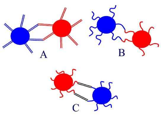
Figure 2.1: Graphical depiction of various schemes for DNA bridging.  A) A freely-jointed, rigid bridge constructed from complementary linker DNA.  B) A flexible bridge can be constructed using complementary linker DNA.  C) A rigid bridge constructed from short, flexible linker DNA and a long, rigid linker.  

The plan for the chapter is as follows.  In section 2.2 we provide a description of the problem.  In section 2.3 we determine the bridging probability for the formation of a DNA bridge between two colloids, assuming the known thermodynamic parameters of DNA(hybridization free energy $\Delta G$).  Using this bridging probability as input, in section 2.4 we calculate the effective binding free energy $\epsilon_{AB}$ for the formation of a dimer.  Section 2.5 establishes the connection between the theory and the experimentally determined melting profile $f(T)$, the fraction of unbound particles as a function of temperature.  In particular, we demonstrate how knowledge of $\epsilon_{AB}$ can be used to determine this profile, including the effects of particle aggregation.  In section 2.6 the theory is compared with two recent experiments detailing the reversible aggregation of colloids with DNA-mediated attraction [2], [1].  Section 2.7 presents a detailed description of how the results can be applied to fit the experimental melting curves for a binary system of DNA-grafted colloids.  The main results of the model are summarized in section 2.8.

2.2 Description of the Problem

We consider particles of type $A$ and $B$ which form reversible $AB$ bonds as a result of DNA hybridization.  The task at hand is to determine the relative abundance of the various colloidal structures that form as a function of temperature.  From this information we can determine which factors affect the melting and aggregation properties in DNA-colloidal assemblies.  To do so we must determine the binding free energy for all of the possible phases(monomer, dimer, …, infinite aggregate), and then apply the rules for thermodynamic equilibrium.  As we will see, these binding free energies can all be simply related to $\epsilon_{AB}$, the binding free energy for the formation of a dimer.  Our task is thus reduced to determining $\epsilon_{AB}$ from the thermodynamic parameters of DNA and structural properties of the DNA linkers.  In our statistical mechanical framework, $\epsilon_{AB}$ is calculated from the model partition function, taking into account the appropriate ensemble averaging for the non-ergodic degrees of freedom.  The result is related to the bridging probability for a pair of linkers.  By considering the specific properties of the DNA bridge that forms, the bridging probability can be related to the hybridization free energy $\Delta G$ of the DNA.  In this way, we obtain a direct link between DNA thermodynamics and the global aggregation and melting properties in colloidal-DNA systems.

2.3 Bridging Probability

To begin we relate the hybridization free energy $\Delta G$ for the DNA in solution to the bridging probability for a pair of linkers.  This bridging probability is defined as the ratio $\frac{P_{bound}}{P_{free}}$, with $P_{bound}$ the probability that the pair of linkers have hybridized to form a DNA bridge, and $P_{free}$ the probability that they are unbound.  This ratio is directly related to the free energy difference of the bound and unbound states of the linkers $\Delta\widetilde{G}$ (throughout this thesis we will use units with $k_{B}=1$):

$$\frac{P_{bound}}{P_{free}} =\exp\left[\frac{-\Delta\widetilde{G}}{T}\right]=\frac{c_{eff}}{c_{o}}\exp\left[\frac{-\Delta G}{T}\right]$$ (2.1)

$$c_{eff} =\frac{\int P(\mathbf{r}_{1},\mathbf{r})P(\mathbf{r}_{2},\mathbf{r})d^{3}\mathbf{r}}{\left(\int P(\mathbf{r},\mathbf{r}^{\prime})d^{3}\mathbf{r}\right)^{2}}$$ (2.2)

Here $c_{o}=1M$ is a reference concentration.  $P(\mathbf{r},\mathbf{r}^{\prime})$ is the probability distribution function for the linker chain which starts at $\mathbf{r}^{\prime}$ and ends at $\mathbf{r}$. The overlap density $c_{eff}$ is a measure of the change in conformational entropy of the linker DNA as a result of hybridization.  It will depend on the properties of the linker DNA(ex: flexible vs. rigid), and the scheme for DNA bridging(ex: hybridization of complementary ends vs. hybridization mediated by an additional linker). $\ c_{eff}$ is the concentration of free DNA which would have the same hybridization probability as the grafted linkers in our problem.  As discussed in section 2.6, the DNA linker grafting density also plays an important role in determining the possible linker configurations and hence $c_{eff}$.

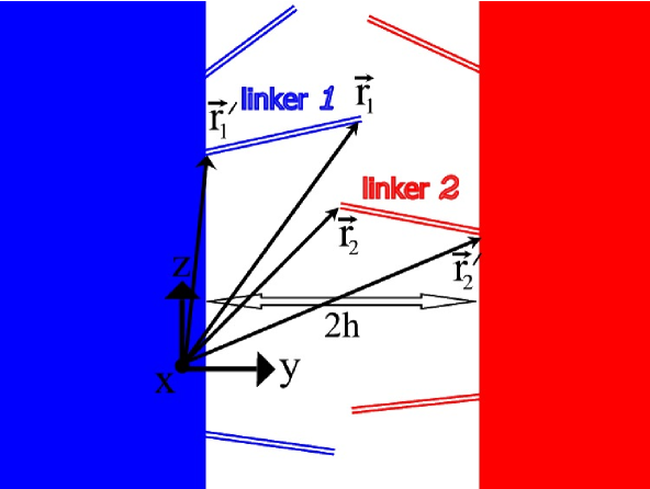
Figure 2.2: The statistical weight of a bound state is calculated by determining the number of hybridized configurations for two complementary linker chains relative to the number of unhybridized configurations.  

Assuming that the size of the linkers is much smaller than the particle radius $R$, we first consider the problem in a planar geometry. Let the two linkers be attached to two parallel planar surfaces separated by a distance $2h$.  Referring to figure 2.2 we see that $\mathbf{r}^{\prime}$ is the location where the linker DNA is grafted onto the particle surface, and $\mathbf{r}$ is the position of the free end.

2.3.1 Hybridization Scheme A: Freely-Jointed Rigid Linkers

In this section we consider hybridization by complementary, rigid linker DNA (scheme A in Figure 2.1).  This scheme is particularly interesting since it is directly related to several recent experiments [1], [2].  We assume that $L<l_{p}$ and $L\ll R$, where $l_{p}\simeq 50nm$ is the persistence length of ds DNA and $L$ is the ds linker DNA length. In this regime, the linker chains can be treated as rigid rods tethered on a planar surface.  The interaction is assumed to be point-like, in which a small fraction $\Delta/L$ of the linker bases hybridize.

We can calculate the overlap density by noting that the integral in Eq. (2.2) is proportional to the volume of intersection of two spherical shells (red and blue circles in Figure 2.3) :

$$c_{eff}=\frac{2\pi rA}{\left(2\pi L^{2}\Delta\right)^{2}}=\frac{\Theta\left(L-\left|\mathbf{r}_{1}^{\prime}-\mathbf{r}_{2}^{\prime}\right|/2\right)}{2\pi L^{2}\left|\mathbf{r}_{1}^{\prime}-\mathbf{r}_{2}^{\prime}\right|},$$ (2.3)

here $A=\Delta^{2}/\sin\beta\$and $r=\sqrt{L^{2}-\left|\mathbf{r}_{1}^{\prime}-\mathbf{r}_{2}^{\prime}\right|^{2}/4}$ (see notations in Figure 2.3). We have used the fact that $\cos\beta/2=\left|\mathbf{r}_{1}^{\prime}-\mathbf{r}_{2}^{\prime}\right|/2L$. $\ c_{eff}$ and the binding probability are largest when the linkers are grafted right in front of each other, i.e. when $\left|\mathbf{r}_{1}^{\prime}-\mathbf{r}_{2}^{\prime}\right|\sim 2h$.  By taking the limit $h\approx L$ we arrive at the following result for the corresponding ”bridging” free energy

$$\Delta\widetilde{G}_{A}\approx\Delta G_{A}+T\log\left[4\pi L^{3}c_{o}\right].$$ (2.4)

This free energy remains nearly constant for any pair of linkers, as long as they can be connected in principle, i.e. $\left|\mathbf{r}_{1}^{\prime}-\mathbf{r}_{2}^{\prime}\right|<2L$. This limits the maximum lateral displacement of the linkers:  $r_{\bot}<2\sqrt{L^{2}-h^{2}}$, and therefore sets the effective cross-section of the interaction:

$$a=\mathbf{\ }\pi r_{\bot}^{2}=4\pi\left(L^{2}-h^{2}\right)$$ (2.5)

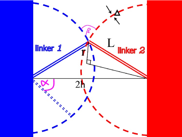
Figure 2.3: Cross-sectional view of the hybridization of two complementary rigid linker DNA.  The overlap density is calculated in a planar approximation to the particle surface.  

2.3.2 Hybridization Scheme B: Complementary Flexible Linkers

We will now consider scenario B of figure 2.1, hybridization of complementary, flexible linker DNA.  This situation can be realized in experiment by choosing linker DNA(ss or ds), provided the chain length $L>>l_{p}$, the persistence length.  We perform the calculation in a planar approximation to the particle surface, which implies the particle radius $R>>R_{g}$, the radius of gyration of the linker chain.  In scenario B, we must also take into account the entropic repulsion $G_{rep}$ of the linker DNA which arises as a result of confining the chains between planar surfaces.  Since we are working with Gaussian chains, we can use the result of Dolan and Edwards [67].  Making the appropriate modification to equation 2.1 the binding probability for a pair of linkers is the following.

$$\exp\left[\frac{-\Delta\widetilde{G}_{B}}{T}\right]=\frac{c_{eff}}{c_{o}}\exp\left[\frac{-(\Delta G_{B}+2G_{rep})}{T}\right]$$ (2.6)

Defining $x\equiv\frac{h}{R_{g}}$ with the planar surfaces separated by a distance $2h$, the free energy of repulsion has the following asymptotic behavior.

$$G_{rep} = -T\log\left[\frac{1}{2x}\sqrt{\frac{8\pi}{3}}\sum_{k=1\text{, }k\text{\ }odd}^{\infty}\exp\left[-\frac{\pi^{2}k^{2}}{24x^{2}}\right]\right]$$ (2.7)

$$\simeq T\left[\log\left(2x\sqrt{\frac{3}{8\pi}}\right)+\frac{\pi^{2}}{24x^{2}}\right]\text{ \ \ }x\ll 1$$ (2.8)

$$G_{rep} = -T\log\left[1-2\sum_{k=1}^{\infty}(-1)^{k+1}\exp\left[-6x^{2}k^{2}\right]\right]$$ (2.9)

$$\simeq -T\log\left[1-2\exp\left(-6x^{2}\right)\right]\text{ \ \ }x\gg 1$$ (2.10)

The details of the calculation are given in Appendix 1.  The final result gives the behavior of the binding probability $\exp\left[\frac{-\Delta\widetilde{G}_{B}}{T}\right]$ between complementary, flexible linkers as a function of $x$ and the separation between grafting points $\mathbf{\Delta r}^{\prime}=\mathbf{r}_{1}^{\prime}-\mathbf{r}_{2}^{\prime}$.

$$\Delta\widetilde{G}_{B} \simeq \Delta G_{B}+T\left[\begin{array}[]{c}\frac{3}{4}\left(\frac{\Delta r^{{}^{\prime}}}{R_{g}}\right)^{2}+\log\left(R_{g}^{3}c_{o}\right)+\log\left(\frac{32}{\pi^{2}}\right)\\ +3\log(x)+\frac{\pi^{2}}{12x^{2}}\end{array}\right]\text{ for\ \ }x\ll 1$$ (2.13)

$$\Delta\widetilde{G}_{B} \simeq \Delta G_{B}+T\left[\begin{array}[]{c}\frac{3}{4}\left(\frac{\Delta r^{{}^{\prime}}}{R_{g}}\right)^{2}+\log\left(R_{g}^{3}c_{o}\right)-\log\left(\frac{9}{4}\sqrt{\frac{3}{\pi}}\right)\\ -2\log(x)+3x^{2}\end{array}\right]\text{ \ for\ }x\gg 1$$ (2.16)

Interpolating between the two regimes, we can see from the figure that the minimum free energy is at $x\lesssim 1$.

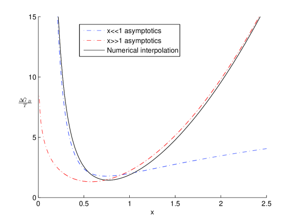
Figure 2.4: $\frac{\Delta\widetilde{G}_{B}(\mathbf{\Delta r}^{{}^{\prime}}=0)}{T}$ as a function of $x$ for flexible DNA bridges.  The figure is normalized by choosing $\frac{\Delta G_{B}}{T}+\log(R_{g}^{3}c_{o})=0$.   

2.3.3 Hybridization Scheme C: Short Flexible Markers with a Long Rigid Linker

We now turn our attention to scenario C of figure 2.1, hybridization of short, flexible marker DNA with radius of gyration $R_{g}$ to a long, rigid linker DNA of length $L$.  We will consider the case $\zeta\equiv\frac{L}{R_{g}}\gg 1$.  For this reason we can neglect the entropic repulsion $G_{rep}$ of the short linkers, since they only feel the presence of the surface to which they are attached.  However, in this scenario we must take into account the loss of entropy of the long, rigid DNA linker.  After hybridization this linker strand does not have the full $4\pi$ steradians of rotational freedom it does when free in solution.  The appropriate modification to the binding probability is:

$$\exp\left[\frac{-\Delta\widetilde{G}_{C}}{k_{B}T}\right] = \frac{c_{eff}}{c_{o}}\exp\left[\frac{-\Delta G_{C}}{k_{B}T}\right]$$ (2.17)

$$c_{eff} = \frac{1}{4\pi L^{2}}\frac{\int P(\mathbf{r}_{1},\mathbf{r}_{1}^{\prime})P(\mathbf{r}_{2},\mathbf{r}_{2}^{\prime})\delta(|\mathbf{r}_{1}-\mathbf{r}_{2}|-L)d^{3}\mathbf{r}_{1}d^{3}\mathbf{r}_{2}}{\left(\int P(\mathbf{r},\mathbf{r}^{\prime})d^{3}\mathbf{r}\right)^{2}}$$ (2.18)

Once again, the reader interested in the details of the calculation is directed to Appendix B.  For completeness we quote the result here.

$$\Delta\widetilde{G}_{C}(\mathbf{\Delta r}^{{}^{\prime}} = 0,\epsilon=\epsilon^{\ast})\simeq\Delta G_{C}+T\log\left[\frac{8\sqrt{\frac{\pi}{3}}L^{2}R_{g}c_{o}}{\left(e^{-\frac{3}{2}}-e^{-\frac{9}{4}}\right)}\right]$$ (2.19)

$$= \Delta G_{C}+4.24T+T\log\left[L^{2}R_{g}c_{o}\right]$$ (2.20)

2.4 Effective Binding Free Energy

We now proceed with the calculation of the effective free energy $\epsilon_{AB}$ , which is associated with the formation of a dimer from a pair of free particles, $A$ and $B$.  Since the DNA coverage on the particle surface is not uniform, this free energy, and the corresponding partition function $Z$, would in principle depend on the orientations of the particles with respect to the line connecting their centers. The equilibrium binding free energy would correspond to the canonical ensemble of all possible orientations, i.e. $\epsilon_{AB}=-T\log 4\pi\left\langle Z\right\rangle$. However, this equilibrium can only be achieved after a very long time, when the particle pair samples all possible binding configurations, or at least their representative subset. The real situation is different. After the first DNA-mediated bridge is created the particle pair can still explore the configurational space by rotating about this contact point. However, after the formation of two or more DNA bridges (at certain relative orientation of the particles), further exploration requires multiple breaking and reconnecting of the DNA links, which is a very slow process. We conclude that the system is ergodic with respect to the various conformations of the linker DNA for fixed orientations of the particles, but the orientations themselves are non-ergodic variables. The only exceptions are the single-bridge states: the system quickly relaxes to a more favorable orientational state (unless the DNA coverage is extremely low, and finding a second contact is very hard).   If $N$ denotes the number of DNA bridges constituting the $AB$ bond, the appropriate expression for $\epsilon_{AB}$ in this partially ergodic regime is the so-called component averaged free energy [68], [69]:

$$\epsilon_{AB}=-T\left\langle\log Z\right\rangle_{N\geq 2}$$ (2.21)

Each DNA bridge between particles can be either open or closed.

$$Z_{bridge}=1+\exp\left(-\frac{\Delta\widetilde{G}(h^{\prime},\mathbf{r}_{1}^{\prime}-\mathbf{r}_{2}^{\prime})}{T}\right)$$ (2.22)

Here $\mathbf{r}_{i}^{\prime}$ is the 2D position where the bridge is grafted onto surface $i$.  We now consider a generic case when the interaction free energy $\Delta\widetilde{G}$ depends on the separation between planar surfaces $2h^{\prime}$, and the separation of grafting points $\mathbf{r}_{1}^{\prime}-\mathbf{r}_{2}^{\prime}$, without assumption of a particular bridging scheme.  If the probability for bridge formation is small, two DNA linkers on the same surface will not compete for complementary linkers.  In this regime the free energy can be calculated by summing over the contribution from each bridge that forms between dimers.

$$F=-T\sum_{i}\sum_{j}\log\left[1+\exp\left(-\frac{\Delta\widetilde{G}(h^{\prime},\mathbf{r}_{i}^{\prime}-\mathbf{r}_{j}^{\prime})}{T}\right)\right]$$ (2.23)

We convert the summation to integration by introducing the linker areal grafting density $\sigma$.

$$F=-T\int\int\sigma_{1}(\mathbf{r}_{1}^{\prime})\sigma_{2}(\mathbf{r}_{2}^{\prime})\log\left[1+\exp\left(-\frac{\Delta\widetilde{G}(h^{\prime},\mathbf{r}_{1}^{\prime}-\mathbf{r}_{2}^{\prime})}{T}\right)\right]d^{2}\mathbf{r}_{1}^{\prime}d^{2}\mathbf{r}_{2}^{\prime}$$ (2.24)

Changing variables to $\mathbf{\Delta r}=\mathbf{r}_{1}^{\prime}-\mathbf{r}_{2}^{\prime}$ and $\mathbf{\rho}=\left(\mathbf{r}_{1}^{\prime}+\mathbf{r}_{2}^{\prime}\right)/2$, we can reintroduce the notion of a bridging cross-section $a(h^{\prime})$, this time in a model-independent manner:

$$a(h^{\prime})\log\left[1+\exp\left(-\frac{\Delta\widetilde{G}_{o}(h^{\prime})}{T}\right)\right]\equiv\int d^{2}\mathbf{\Delta r}\log\left[1+\exp\left(-\frac{\Delta\widetilde{G}(h^{\prime},\mathbf{\Delta r})}{T}\right)\right]$$ (2.25)

Here $\Delta\widetilde{G}_{o}(h^{\prime})\equiv\Delta\widetilde{G}(h^{\prime},\mathbf{\Delta r}=0)$ is the minimum free energy with respect to the separation between grafting points $\mathbf{\Delta r}$. We can now write the free energy:

$$F=-T\int\sigma_{1}(\overrightarrow{\mathbf{\rho}})\sigma_{2}(\overrightarrow{\mathbf{\rho}})a(h^{\prime})\log\left[1+\exp\left(-\frac{\Delta\widetilde{G}_{o}(h^{\prime})}{T}\right)\right]d^{2}\mathbf{\rho}$$ (2.26)

We now convert from the planar geometry to the spherical particle geometry using the Derjaguin approximation [70].

$$d^{2}\mathbf{\rho} =\rho d\rho d\phi$$ (2.27)

$$h^{\prime} =h+\frac{\rho^{2}}{2R}$$ (2.28)

Let $\Delta\widetilde{G}_{\ast}$  be the minimal value of the bridging free energy.   Then the result for $F$ can be rewritten as:

$$F=-TN\log\left[1+\exp\left(-\frac{\Delta\widetilde{G}_{\ast}}{T}\right)\right]$$ (2.29)

Here $N$ has a physical meaning as the number of potential bridges for given relative positions and orientations of the particles:

$$N\equiv\int\sigma_{1}(\overrightarrow{\mathbf{\rho}})\sigma_{2}(\overrightarrow{\mathbf{\rho}})a(h^{\prime})\left(\frac{\log\left[1+\exp\left(-\Delta\widetilde{G}_{o}(h^{\prime})/T\right)\right]}{\log\left[1+\exp\left(-\Delta\widetilde{G}_{\ast}/T\right)\right]}\right)d^{2}\mathbf{\rho}$$ (2.30)

One can calculate the average value of $N$ in terms of the average grafting density, $\sigma=\left\langle\sigma_{1}\right\rangle=\left\langle\sigma_{2}\right\rangle:$

$$\left\langle N\right\rangle\equiv 2\pi R\sigma^{2}\int a(h^{\prime})\left(\frac{\log\left[1+\exp\left(-\Delta\widetilde{G}_{o}(h^{\prime})/T\right)\right]}{\log\left[1+\exp\left(-\Delta\widetilde{G}_{\ast}/T\right)\right]}\right)dh^{\prime}$$ (2.31)

In a generic case of randomly grafted linkers, $\left\langle N\right\rangle$ completely defines the overall distribution function of $N$, which must have a Poisson form: $P(N)=\frac{\left\langle N\right\rangle^{N}e^{-\left\langle N\right\rangle}}{N!}$.  The average number of bridges $\left\langle N\right\rangle$ between two particles depends on both the DNA linker grafting density $\sigma$ and the bridging probability determined from $\Delta\widetilde{G}$.

The free energy for the formation of a dimer $\epsilon_{AB}=\left\langle F\right\rangle_{2+}-T\log\Omega$.  The second term is the entropic contribution to the free energy, which comes from integration over the orientational and translational degrees of freedom of the second particle.  Because the system is not ergodic in these degrees of freedom, the accessible phase space $\Omega$ will be reduced by a factor of $P_{2+}$. $\ P_{2+}$ is the probability that there are at least two DNA bridges between the particles.  In terms of the average number of bridges $\left\langle N\right\rangle$ between particles, we have the following relations:

$$P_{2+} =1-(1+\left\langle N\right\rangle)e^{-\left\langle N\right\rangle}$$ (2.32)

$$\left\langle N\right\rangle_{2+} =\frac{\left\langle N\right\rangle\left(1-e^{-\left\langle N\right\rangle}\right)}{P_{2+}}$$ (2.33)

$$\epsilon_{AB}=-T\left\{\left\langle N\right\rangle_{2+}\log\left[1+\exp\left(-\frac{\Delta\widetilde{G}_{\ast}}{T}\right)\right]+\log\left[P_{2+}4\pi\delta(2R)^{2}c_{o}\right]\right\}$$ (2.34)

Here $\delta$ is the localization length of the $AB$ bond, which comes from integrating the partition function over the radial distance between particles.

2.4.1 Scheme A

We now can calculate $\left\langle N\right\rangle$ for the case of freely-jointed rigid bridging considered earlier (i.e. for scheme A).  In a previous section we provided a direct calculation of the interaction free energy, $\Delta\widetilde{G}_{o}\left(h\right)\approx const=\Delta\widetilde{G}_{\ast}$ (eq.2.4), and bridging cross-section, $a(h^{\prime})=4\pi(L^{2}-h^{\prime 2})$. Applying eq. 2.31 we arrive immediately at the following result.

$$\left\langle N\right\rangle=8\pi^{2}\sigma^{2}R\int\limits_{0}^{L}(L^{2}-h^{\prime 2})dh^{\prime}=\frac{16\pi^{2}\sigma^{2}RL^{3}}{3}$$ (2.35)

2.4.2 Scheme B

We note that in this case, since the binding probability for a given pair of linkers is Gaussian in the separation between grafting points $\mathbf{\Delta r}=\mathbf{r}_{1}^{\prime}-\mathbf{r}_{2}^{\prime}$, we can perform an analytic calculation of the effective cross section.  In what follows $x^{\prime}=h^{\prime}/R_{g}$.  Recall the definition of $a(h^{\prime})$:

$$a(h^{\prime})\log\left[1+\exp\left(\frac{-\Delta\widetilde{G}_{o}(h^{\prime})}{T}\right)\right]=\mathop{\displaystyle\int}d^{2}\mathbf{\Delta r}\log\left[1+\exp\left(\frac{-\Delta\widetilde{G}_{B}(h^{\prime},\mathbf{\Delta r})}{T}\right)\right]$$ (2.36)

$$\exp\left[\frac{-\Delta\widetilde{G}_{B}(\mathbf{\Delta r})}{T}\right]=\Lambda(x^{\prime})\exp\left[-\frac{3}{4}\left(\frac{\mathbf{\Delta r}}{R_{g}}\right)^{2}\right]$$ (2.37)

$$\Lambda(x^{\prime})\equiv\frac{c(x^{\prime})}{R_{g}^{3}c_{o}}\exp\left[\frac{-(\Delta G_{B}+2G_{rep})}{T}\right]$$ (2.38)

The explicit form of the dimensionless concentration $c(x^{\prime})$ is given in Appendix A (see Eq. A.11).  Changing to polar coordinates $(r,\theta)$ we have:

$$a(x^{\prime})\log\left[1+\Lambda(x^{\prime})\right]=\mathop{\displaystyle\int}_{0}^{2\pi}d\theta\mathop{\displaystyle\int}\limits_{0}^{\infty}r\log\left[1+\Lambda(x^{\prime})\exp\left[-\frac{3}{4}\left(\frac{r}{R_{g}}\right)^{2}\right]\right]dr$$ (2.39)

Define a new variable $u(r)\equiv\Lambda(x^{\prime})\exp\left[-\frac{3}{4}\left(\frac{r}{R_{g}}\right)^{2}\right]$.

$$a(x^{\prime})\log\left[1+\Lambda(x^{\prime})\right]=-\frac{4\pi}{3}R_{g}^{2}\mathop{\displaystyle\int}\limits_{\Lambda(x^{\prime})}^{0}du\frac{\log\left[1+u\right]}{u}=-\frac{4\pi}{3}R_{g}^{2}Li_{2}\left[-\Lambda(x^{\prime})\right]$$ (2.40)

The calculation yields the following result, with $Li_{2}\left[z\right]\equiv\mathop{\displaystyle\sum}\limits_{k=1}^{\infty}\frac{z^{k}}{k^{2}}$ the Dilogarithm.

$$a(x^{\prime})=-\frac{4\pi}{3}\frac{Li_{2}\left[-\Lambda(x^{\prime})\right]}{\log\left[1+\Lambda(x^{\prime})\right]}R_{g}^{2}$$ (2.41)

Since $Li_{2}(z)<0$ for $z<0$, $a(x^{\prime})$ is positive as required.  From this effective cross section we can compute the average free energy $\left\langle F\right\rangle$ as a result of DNA bridging between particles, with $\sigma$ the average areal grafting density of DNA linkers.  Here $\mathbf{\rho}=\mathbf{r}_{1}^{{}^{\prime}}+\mathbf{r}_{2}^{{}^{\prime}}$, with $\mathbf{r}_{i}^{{}^{\prime}}$ the location where linker $i$ is grafted on the planar surface.

$$\left\langle F\right\rangle=-T\sigma^{2}\mathop{\displaystyle\int}a(x^{{}^{\prime}})\log\left[1+\Lambda(x^{{}^{\prime}})\right]d^{2}\mathbf{\rho}$$ (2.42)

Converting from the planar geometry to the spherical nanoparticle geometry using the Derjaguin approximation we have:

$$x^{{}^{\prime}}=x+\frac{\rho^{2}}{2RR_{g}}$$ (2.43)

$$\left\langle F\right\rangle=T\frac{8\pi^{2}}{3}\sigma^{2}RR_{g}^{3}\mathop{\displaystyle\int}\limits_{0}^{\infty}Li_{2}\left[-\Lambda(x^{{}^{\prime}})\right]dx^{{}^{\prime}}$$ (2.44)

This integration can be performed numerically.  As discussed previously, the free energy $\epsilon_{AB}$ for the formation of a dimer($AB$ pair) also contains an entropic contribution from integration over the orientational and translational degrees of freedom of the second particle.

2.4.3 Scheme C

We can also determine the free energy in this scenario using the approximation method developed.

$$F=-T\left\langle N\right\rangle\log\left[1+\exp\left(-\frac{\Delta\widetilde{G}_{C}(\mathbf{\Delta r}^{{}^{\prime}}=0,\epsilon=\epsilon^{\ast})}{T}\right)\right]$$ (2.45)

We provide a simple geometrical argument to determine the average number of DNA bridges $\left\langle N\right\rangle$ between particles.  We assume that the rigid linkers are aligned with a small component parallel to the surface.

$$a(h) \simeq \pi y^{2}$$ (2.46)

$$y = (L+\Delta)\tan\theta_{\max}\approx R_{g}(1+\epsilon)$$ (2.47)

Then applying equation 2.31 with $h=\frac{L}{2}(1+\epsilon)$ we have:

$$\left\langle N\right\rangle=\pi^{2}\sigma^{2}RR_{g}^{2}L\mathop{\displaystyle\int}\limits_{0}^{2\epsilon^{\ast}}(1+\epsilon)^{2}d\epsilon\simeq 2\sqrt{2}\pi^{2}\sigma^{2}RR_{g}^{3}$$ (2.48)

2.5 Aggregation and Melting Behavior

At this stage we have calculated the binding free energy $\epsilon_{AB}$ for an $AB$ pair, starting with the thermodynamic parameters of DNA (hybridization free energy $\Delta G$).  In this section we establish the connection between that result and the experimentally observable morphological behavior of a large system. One of the ways to characterize the system is to study its melting profile $f(T)$, which is the fraction of unbound particles as a function of temperature.  To determine the profile we calculate the chemical potential for each phase(monomer, dimer, etc.) and apply the thermodynamic rules for phase equilibrium.  We will demonstrate how the single binding free energy $\epsilon_{AB}$ can be used to determine the contribution of each phase to the melting profile, including the effects of aggregation.

2.5.1 Dimer Formation

To begin we discuss the formation of dimers via the reaction $A+B\rightleftharpoons AB$.  We can express the chemical potential of the $i^{th}$ species $\mu_{i}$ in terms of the particle concentrations $c_{i}=\frac{N_{i}}{V}$.

$$\mu_{A} =T\log\left(c_{A}\right)$$ (2.49)

$$\mu_{B} =T\log\left(c_{B}\right)$$ (2.50)

$$\mu_{AB} =T\log\left(c_{AB}\right)+\epsilon_{AB}$$ (2.51)

Here $\epsilon_{AB}$ is the binding free energy for the formation of a dimer.  In terms of the potential $V(r)$ between $A$ and $B$ type particles we have:

$$\epsilon_{AB}=-T\log\left[4\pi(2R)^{2}c_{o}\int dr\exp\left(-\frac{V(r)}{T}\right)\right]$$ (2.52)

In this section we are not particularly concerned with the specific form of the DNA-induced potential $V(r)$, having already determined $\epsilon_{AB}$ in the previous section.  We simply note that the prefactor $4\pi(2R)^{2}$ arises since the interaction is assumed to be isotropic, with $R$ the particle radius.  Equilibrating the chemical potential of the various particle species, we obtain the condition for chemical equilibrium.   

$$\mu_{A}+\mu_{B}=\mu_{AB}$$ (2.53)

The result is a relationship between the concentration of dimers and monomers.

$$c_{AB}=\frac{c_{A}c_{B}}{c_{o}}\exp\left[\frac{-\epsilon_{AB}}{T}\right]$$ (2.54)

The overall concentration of particles in monomers and dimers must not differ from the initial concentration.

$$c_{A}^{i} =c_{A}+c_{AB}$$ (2.55)

$$c_{B}^{i} =c_{B}+c_{AB}$$ (2.56)

If the system is prepared at equal concentration, $c_{A}^{i}=c_{B}^{i}=\frac{1}{2}c_{tot}$, subtracting the two equations we see that $c_{A}=c_{B}\equiv c$.  Written in terms of the fraction of unbound particles $f=\frac{c}{\frac{1}{2}c_{tot}}$ we have a quadratic equation for the unbound fraction.

$$1=f+\exp\left[\frac{-\widetilde{\epsilon}_{AB}}{T}\right]f^{2}$$ (2.57)

To simplify we have defined an effective free energy $\widetilde{\epsilon}_{AB}$ for the formation of a dimer.

$$\widetilde{\epsilon}_{AB}=\epsilon_{AB}-T\log\left[\frac{c_{tot}}{2c_{o}}\right]$$ (2.58)

The solution for the fraction of unbound particles as a function of temperature is simply:

$$f=\frac{-1+\sqrt{1+4\exp\left[\frac{-\widetilde{\epsilon}_{AB}}{T}\right]}}{2\exp\left[\frac{-\widetilde{\epsilon}_{AB}}{T}\right]}$$ (2.59)

Previous studies[1] only included the dimer contribution to the melting properties of DNA colloidal assemblies.  With the basic formalism at hand, we can now extend the preceding analysis to include the contribution of trimers and tetramers.

2.5.2 Trimers and Tetramers

Now consider the formation of a trimer via $2A+B\rightleftharpoons ABA$.  The chemical potential is slightly different in this case.

$$\mu_{ABA}=T\log\left(c_{ABA}\right)+\epsilon_{ABA}$$ (2.60)

Taking into account that there are now two $AB$ bonds in the structure, one might conclude that $\epsilon_{ABA}=2\epsilon_{AB}$.  This is not quite correct, since there is a reduction in solid angle available to the third particle.  To form a trimer, an $AB$ bond forms first, which contributes $\epsilon_{AB}$ to $\epsilon_{ABA}$.  Some simple geometry shows that the remaining $A$ particle only has $3\pi$ steradians of possible bonding sites to particle $B$.  Making this change in the prefactor of eq. 2.52, one can see that the second bond contributes $\epsilon_{AB}-T\log\left(\frac{3}{4}\right)$ to $\epsilon_{ABA}$.

$$\epsilon_{ABA}=2\epsilon_{AB}-T\log\left(\frac{3}{4}\right)$$ (2.61)

The equation for chemical equilibrium can once again be expressed in terms of the particle concentrations.

$$2\mu_{A}+\mu_{B} =\mu_{ABA}$$ (2.62)

$$c_{ABA} =\frac{3}{4}\frac{c_{A}^{2}c_{B}}{c_{o}^{2}}\exp\left[\frac{-2\epsilon_{AB}}{T}\right]$$ (2.63)

To include the trimer contribution, we note that there are two possible varieties, with $\epsilon_{ABA}=\epsilon_{BAB}$.

$$c_{A}^{i} =c_{A}+c_{AB}+2c_{ABA}+c_{BAB}$$ (2.64)

$$c_{B}^{i} =c_{B}+c_{AB}+c_{ABA}+2c_{BAB}$$ (2.65)

Following the same line of reasoning as before, the resulting equation for the unbound fraction $f$ is:

$$1=f+\exp\left[\frac{-\widetilde{\epsilon}_{AB}}{T}\right]f^{2}+\frac{9}{4}\exp\left[\frac{-2\widetilde{\epsilon}_{AB}}{T}\right]f^{3}$$ (2.66)

For tetramers we will follow the same general reasoning, however in this case there are two different structure types.  The reaction $2A+2B\rightleftharpoons ABAB$ results in the formation of string like structures.

$$\mu_{ABAB}=T\log\left(c_{ABAB}\right)+\epsilon_{ABAB}$$ (2.67)

As in the trimer case, the last particle has $3\pi$ steradians of possible bonding sites, and contributes $\epsilon_{AB}-T\log\left(\frac{3}{4}\right)$ to $\epsilon_{ABAB}$.

$$\epsilon_{ABAB} =3\epsilon_{AB}-T\log\left[\left(\frac{3}{4}\right)^{2}\right]$$ (2.68)

$$2\mu_{A}+2\mu_{B} =\mu_{ABAB}$$ (2.69)

$$c_{ABAB} =\left(\frac{3}{4}\right)^{2}\frac{c_{A}^{2}c_{B}^{2}}{c_{o}^{3}}\exp\left[\frac{-3\epsilon_{AB}}{T}\right]$$ (2.70)

If an $A$ type particle approaches a trimer of variety $ABA$, a branched structure can result.  The reaction $3A+B\rightleftharpoons AAAB$ results in the formation of these branched structures.

$$\mu_{AAAB}=T\log\left(c_{AAAB}\right)+\epsilon_{AAAB}$$ (2.71)

For the branched case, the last particle has approximately $2\pi$ steradians of possible bonding sites, and contributes $\epsilon_{AB}-T\log\left(\frac{1}{2}\right)$ to $\epsilon_{AAAB}$.

$$\epsilon_{AAAB} =3\epsilon_{AB}-T\log\left(\frac{3}{8}\right)$$ (2.72)

$$3\mu_{A}+\mu_{B} =\mu_{AAAB}$$ (2.73)

$$c_{AAAB} =\left(\frac{3}{8}\right)\frac{c_{A}^{3}c_{B}}{c_{o}^{3}}\exp\left[\frac{-3\epsilon_{AB}}{T}\right]$$ (2.74)

To include all of the tetramer contributions, note that there are two branched varieties, with $\epsilon_{AAAB}=\epsilon_{BBBA}$.  Finally we impose the constraint that the initial particle concentrations do not differ from the concentration of all the n-mers, for n=1,2,3,4.

$$c_{A}^{i} =c_{A}+c_{AB}+2c_{ABA}+c_{BAB}+2c_{ABAB}+3c_{AAAB}+c_{BBBA}$$ (2.75)

$$c_{B}^{i} =c_{B}+c_{AB}+c_{ABA}+2c_{BAB}+2c_{ABAB}+c_{AAAB}+3c_{BBBA}$$ (2.76)

The final result is an equation for the unbound fraction $f$ expressed entirely in terms of the effective free energy $\widetilde{\epsilon}_{AB}$ of a dimer.

$$1=f+\exp\left[\frac{-\widetilde{\epsilon}_{AB}}{T}\right]f^{2}+\frac{9}{4}\exp\left[\frac{-2\widetilde{\epsilon}_{AB}}{T}\right]f^{3}+\frac{21}{8}\exp\left[\frac{-3\widetilde{\epsilon}_{AB}}{T}\right]f^{4}$$ (2.77)

For high temperatures, the melting profile is governed by the solution to this polynomial equation for $f$.  For temperatures below the melting point we expect to find particles in large extended clusters.  We now proceed to calculate the equilibrium condition between monomers in solution and the aggregate.

2.5.3 Reversible Sol-Gel Transition

To understand the basic structure of the aggregate, we simply note that there are many DNA attached to each particle.  This gives rise to branching, as in the discussion of possible tetramer structures.  Since the DNA which mediate the interaction are grafted onto the particle surface, once two particles are bound, the relative orientation of the pair is essentially fixed.  The resulting aggregate is a tree-like structure, and the transition to an infinite aggregate at low temperatures is analogous to the sol-gel transition in branched polymers [21].

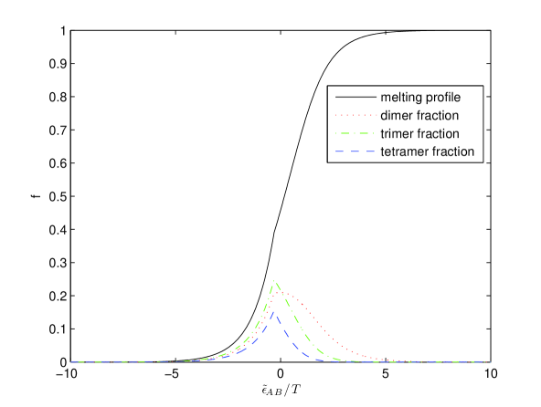
Figure 2.5: The actual unbound fraction $f$ is the concatenation of the aggregate profile for $T<T^{\ast}\$and the n-mer profile for $T>T^{\ast}$.  The fraction of particles in dimers, trimers, and tetramers is also plotted.  

Particles in the aggregate are pinned down by their nearest neighbor bonds, so we do not consider their translational entropy.   As a result the chemical potential is simply $\mu_{\infty}=\epsilon_{\infty}$.  Equilibrating the chemical potential of the monomer in solution and in the aggregate we have:

$$T\log\left(c\right) =\epsilon_{\infty}$$ (2.78)

$$\epsilon_{\infty} =\epsilon_{AB}-T\log\left(\gamma_{\infty}\right)$$ (2.79)

Here $\gamma_{\infty}\simeq 1$ is the configurational entropy of the branched aggregate, per particle.

The concentration of particles in the aggregate $c_{\infty}$ is the the total concentration minus the n-mer concentration.  Here $c_{1}=c_{A}+c_{B}$ is the total monomer concentration, $c_{2}=c_{AB}$ is the total dimer concentration, etc.

$$c_{\infty}\approx c_{tot}-c_{1}-c_{2}-c_{3}-c_{4}$$ (2.80)

Expressed in terms of $\widetilde{\epsilon}_{AB}$ and the fraction of solid angle available to particles in the aggregate $\gamma_{\infty}=\frac{\Omega_{\infty}}{4\pi}$ we have:

$$f_{\infty}=\frac{1}{\gamma_{\infty}}\exp\left[\frac{\widetilde{\epsilon}_{AB}}{T}\right]$$ (2.81)

The transition from dimers, trimers, etc. to the aggregation behavior is the temperature $T^{\ast}$ at which $f_{\infty}(T^{\ast})$ is a solution to eq. 2.77.  In words, $T^{\ast}$ is the temperature at which the aggregate has a non-zero volume fraction.  The fraction of unbound particles for these colloidal assemblies will be governed by eq. 2.81 for $T<T^{\ast}$ and eq. 2.77 for $T>T^{\ast}$.  As claimed, we can simply relate the unbound fraction to $\widetilde{\epsilon}_{AB}$ for both n-mers and the aggregate.

2.6 Comparison to the Experiments

Let’s consider the experimental scheme of Chaikin et al [1].  In the experiment, $R=.5\mu m$ polystyrene beads were grafted with ds DNA linkers of length $L\simeq 20nm$.  The 11 end bases of the $A$ and $B$ type particles were single stranded and complementary.  We have already determined the bridging probability in this scenario(see scheme A).  In the experiment [1] a polymer brush is also grafted onto the particle surface, which will have the effect of preferentially orienting the rods normal to the surface(See Figure 2.3).  This confinement of the linker DNA can be incorporated quite easily into our results for $\Delta\widetilde{G}$ and $\left\langle N\right\rangle$.  To modify Eq. 2.4, when integrating over linker conformations we simply confine each rigid rod to a cone of opening angle $2\alpha$.  The upper bound for the polar integration is now $\alpha$ as opposed to $\pi$.

$$\Delta\widetilde{G}_{A}\simeq\Delta G_{A}+T\log\left[4\pi L^{3}c_{o}(1-\cos\alpha)^{2}\right]$$ (2.82)

The alignment effect should also be taken into account when calculating $\left\langle N\right\rangle$.  If the particles are separated by less than $2L\cos\alpha$ the end sequences will be unable to hybridize.  Following the same steps as before, the lower bound for the $h^{{}^{\prime}}$ integration is now $L\cos\alpha$ as opposed to $0$.

$$\left\langle N\right\rangle =8\pi^{2}\sigma^{2}R\int_{L\cos\alpha}^{L}(L^{2}-h^{{}^{\prime}2})dh^{{}^{\prime}}$$ (2.83)

$$=\frac{16}{3}\pi^{2}\sigma^{2}RL^{3}\left[1+\frac{\cos\alpha}{2}(\cos^{2}\alpha-3)\right]$$ (2.84)

In the absence of the brush, and at sufficiently low linker grafting density $\sigma$, the alignment effect could be removed by setting $\alpha=\frac{\pi}{2}$, in which case we recover our previous results. Since the polymer brush is stiff, it also imposes a minimum separation of $2h$ between particles, where $h$ is the height of the brush.  As a result, in the expression for $\epsilon_{AB}$ we can approximate the radial flexibility of the $AB$ bond as $\delta\simeq L-h$.

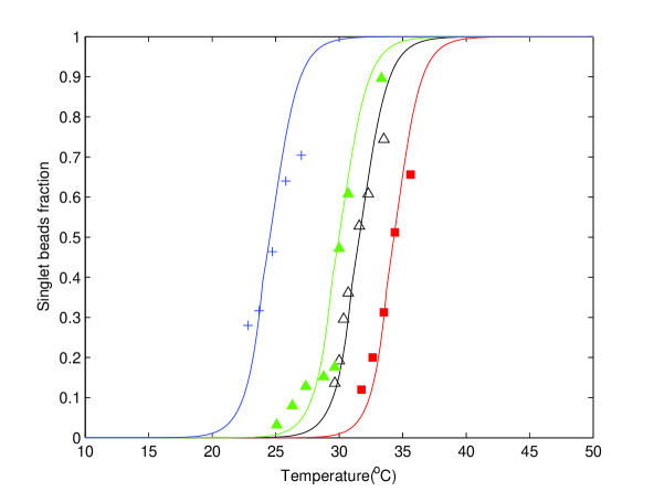
Figure 2.6: Comparison of the melting curves $f(T)$ determined by our model to the experimental data of Chaikin et al(See Fig.2 in [1]).  The four data sets are for the four different polymer brushes used.  For the model fits we find that $\left\langle N\right\rangle_{2+}$=2.01 for crosses, 2.07 for solid triangles, 2.13 for empty triangles, and 2.35 for squares.  

We have now related the free energy $\epsilon_{AB}$ to the known thermodynamic parameters of DNA($\Delta G=\Delta H-T\Delta S$, $\Delta H=-77.2\frac{kcal}{mol}$ and $\Delta S=-227.8\frac{cal}{molK}$), and the properties of linker DNA chains attached to the particles(grafting density $\sigma\simeq 3\times 10^{3}\frac{DNA}{\mu m^{2}}$ and linker length $L\simeq 20nm$).  The height of the polymer brush is $h=13\pm 5nm$ [1].  In fitting the experimental data we have taken the average value $\left\langle h\right\rangle=13nm$.  Changing $h$ within these bounds does not have a major effect on the melting curves.  As a result there is one free parameter in the model, the confinement angle $\alpha$.  This angle determines $\left\langle N\right\rangle$ and $\Delta\widetilde{G}$, which in turn determine $\widetilde{\epsilon}_{AB}$, and finally the melting profile $f$.

With some minor modifications we can also analyze the ”tail to tail” hybridization mode in a recent experiment of Mirkin et al [2].  In this experiment, $R=6.5nm$ gold nanoparticles were chemically functionalized with ss DNA linkers.  The last $15$ bases on the markers for particles of type $A$ and $B$ were chosen to be complementary to a $30$ base ss DNA linker.  Since the strands are not ligated after hybridization, the experimental pictures are similar.

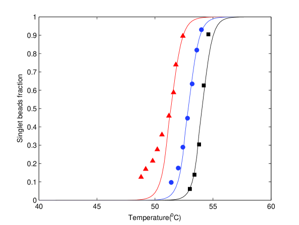
Figure 2.7: The effect of the linker DNA grafting density $\sigma$ on the melting profile$\ f(T)$.  The results of the model are compared with experimental data in [2]. The three data sets represent grafting densities of 100%(squares), 50%(circles), and 33%(triangles) for which $\left\langle N\right\rangle_{2+}$=2.32, 2.16, and 2.05 respectively.  

The unhybridized portion of the ss DNA linker simply serves as a spacer, and the hybridized portions become ds DNA, which we can again treat as rigid rods.  This experiment is done without the addition of a polymer brush, but the grafting density is two orders of magnitude larger than the experiment of Chaikin et al.  As a result, there is still an entropic repulsion [55] associated with compressing the particles below separation $2h$.  Here $h$ could loosely be interpreted as the radius of gyration of the unhybridized portion of the linker.  Despite the fact that $L\sim R$, our planar calculation of $\Delta\widetilde{G}$ provides a good fit to the experimental data.  The other major difference is that now the attraction between particles is mediated by an additional DNA linker.

$$\Delta G=\Delta G_{1}+\Delta G_{2}-T\log\left[\frac{c_{link}}{c_{o}}\right]$$ (2.85)

The term $\Delta G_{1}(\Delta G_{2})$ is the contribution to the free energy from the hybridization of the linker on an $A(B)$ type particle to the complementary portion of the 30 base ss linker.  The hybridization free energies $\Delta G_{1}$ and $\Delta G_{2}$ were calculated with the DINAMelt web server [71].  The last term is the contribution to the free energy from the translational entropy of the additional linker DNA, with $c_{link}$ the additional linker concentration.  This highlights some incorrect assumptions of the thermodynamic melting model [2], where the two hybridization free energies were not calculated separately, and the translational entropy of the additional linker DNA was ignored.  By introducing dilutent strands to the system, one can probe the effect of the linker grafting density $\sigma$ on the melting properties of the assembly(See Figure 2B in [2]).  The agreement between the experimental data and our theory is good, except at small $f$ values.  This is not surprising, since comparing the two requires relating the measurement of optical extinction to the unbound fraction $f$.  This is a nontrivial matter when dealing with aggregation, which corresponds to the small $f$ regime.

2.7 Fitting Algorithm

In this section we present a step by step method for fitting the melting curves obtained experimentally for a binary system of DNA-grafted colloids.

Step 1: Determine $\Delta G$

The first step is to determine the hybridization free energy $\Delta G$ for the DNA strands free in solution.  In many cases the value has been determined experimentally.  Alternatively, there are a number of web based applications which calculate hybridization free energies.  For example, the DINAMelt server which can be located at http://www.bioinfo.rpi.edu/applications/hybrid/hybrid2.php and NUpack which can be located at http://piercelab.caltech.edu/nupack.  Note that in the case where the hybridization is mediated by an additional linker, the translational entropy of that linker must be taken into account (see Eq. 2.85).

Step 2: $\Delta G\rightarrow\Delta\widetilde{G}$

Since the DNA linkers in our problem are grafted onto the particle surface, we need to determine how the grafting effects the bridging probability (see Eqs. 2.1 and 2.2).  This entails calculating the overlap density $c_{eff}$ which is a measure of the change in conformational entropy of the DNA strands upon hybridization.  Determining the appropriate calculation will depend on the hybridization scheme (see Fig. 2.1).  In this chapter calculations have been performed for three different schemes (see Eqs. 2.4, 2.13, 2.19), although the effects of linker confinement have only been taken into account in scheme $A$ (see Eq. 2.82).

Step 3: Calculate $\left\langle N\right\rangle$

The next step in the procedure is to determine the average number of bridges $\left\langle N\right\rangle$ that form between an $AB$ pair.  The general starting point is Eq. 2.31.  In this chapter calculations have been performed for three different hybridization schemes (see Eqs. 2.35, 2.44, 2.48).  The effects of linker confinement have been taken into account in scheme $A$ (see Eq. 2.83).  Note that in our approximation scheme the general relation between $\left\langle N\right\rangle$ and the free energy $F$ is given by Eq. 2.29.

Step 4: Determine $\widetilde{\epsilon}_{AB}$

The next step in the procedure is to relate $\left\langle N\right\rangle$ to the binding energy for the formation of a dimer pair $\epsilon_{AB}$ (see Eq. 2.34).  The quantity of interest for the fitting $\widetilde{\epsilon}_{AB}$ is simply related to $\epsilon_{AB}$ by Eq. 2.58.

Step 5: Determine the melting profile $f(T)$

We are now in a position to relate the calculation to the experimentally measured quantity $f(T)$, which is the fraction of monomers as a function of temperature.  For high temperatures $f$ is determined by the solution of the polynomial Eq. 2.77.  As the temperature is lowered at $T=T^{\ast}$ we reach the point where $f$ determined from the n-mer profile (Eq. 2.77) is equal to $f$ determined from the aggregate profile (Eq. 2.81).  For $T<T^{\ast}$ the melting profile is determined by Eq. 2.81.

2.8 Summary

We have developed a statistical mechanical description of aggregation and melting in DNA-mediated colloidal systems.  First we obtained a general result for two-particle binding energy in terms of DNA hybridization free energy $\Delta G$, and two model–dependent parameters: the average number of available bridges $\left\langle N\right\rangle$ and the overlap density for the DNA $c_{eff}$.  We have also shown how these parameters can be calculated for a particular bridging scheme. In our discussion we have explicitly taken into account the partial ergodicity of the problem related to slow binding-unbinding dynamics.

In the second part it was demonstrated that the fractions of dimers, trimers and other clusters, including the infinite aggregate, are universal functions of a parameter $\ \widetilde{\epsilon}_{AB}/T=\epsilon_{AB}/T-\log\left[c_{tot}/2c_{0}\right]$.  The theory has been calculated for three separate hybridization schemes.  The obtained melting curves are in excellent agreement with two types of experiments, done with particles of nanometer and micron sizes. Furthermore, our analysis of the experimental data give an additional insight into microscopic physics of DNA bridging in these systems: it was shown that the experiments cannot be explained without the introduction of angular localization of linker dsDNA.  The corresponding localization angle $\alpha$ is the only fitting parameter of the model, which allows one to fit both the position and width of the observed melting curves.

There are several manifestations of the greater predictive power of our statistical mechanics approach, compared to the earlier more phenomenological models.  First, once $\alpha$ is determined for a particular system, our theory allows one to calculate the melting behavior for an alternative choice of DNA linker sequences.  Second, if the resulting clusters are separated, for example in a density gradient tube, the relative abundance of dimers, trimers, and tetramers can be compared to the values determined from the theory.

Finally, the theory predicts aging of the colloidal structures, one experimental signature for which is hysteresis of the melting curves.  Such an experiment proceeds by preparing a system above the melting temperature, and measuring the unbound fraction of colloids as the temperature is lowered.  The system is allowed to remain in this cooled state for a very long time, perhaps months, during which multiple DNA bridges break and reform.  During this time the colloids relax into a more favorable orientation state, including states which are not accessible by simply rotating about the contact point formed by the first DNA bridge between particles.  This favorable orientation state is characterized by an average number of DNA bridges $\left\langle N\right\rangle$ greater than what we calculate in the partially ergodic regime.  If the unbound fraction is then measured as the temperature is increased, the melting curve will shift to a higher temperature, consistent with a larger value of $\left\langle N\right\rangle$.

Chapter 3 Dynamics of ”Key-Lock” Interacting Particles

3.1 Introduction

In this chapter [72], [73] we present a theoretical study of desorption and diffusion of particles which interact through key-lock binding of attached biomolecules.  It is becoming common practice to functionalize colloidal particles with single-stranded DNA (ssDNA) to achieve specific, controllable interactions [26], [1], [43], [15], [25], [49].  Beyond the conceptual interest as a model system to study glassiness [65] and crystallization, there are a number of practical applications.  Colloidal self-assembly may provide a fabrication technique for photonic band gap materials [74], [75].  One of the major experimental goals in this line of research is the self-assembly of colloidal crystals using DNA mediated interactions.  The difficulty stems in part from the slow relaxation dynamics in these systems.  The main goal of this chapter is to understand how the collective character of key-lock binding influences the particle dynamics.  In doing so we gain valuable insight into the relaxation dynamics, and propose a modified experimental setup whose fast relaxation should facilitate colloidal crystallization.

Similar systems have also attracted substantial attention in other areas of nanoscience.  In particular, by functionalizing nanoparticles with antibodies to a particular protein, the nanoparticles have potential applications as smart, cell-specific drug delivery vehicles [76], [77].  These nanodevices take advantage of the fact that certain cancerous cells overexpress cell membrane proteins, for example the folate receptor.  An improved understanding of desorption and diffusion on the cell membrane surface may have implications for optimizing the design of these drug delivery vehicles.  This is the subject of chapter 7.

In what follows we present our results on the dynamics of particles which interact through reversible key-lock binding.  The plan for the chapter is the following.  In section 3.2 we introduce the key-lock model and explain the origin of the two model parameters $\Delta$ and $\overline{m}$.  The parameter $\Delta$ determines the binding energy for the formation of a key-lock pair.  The parameter $\overline{m}$ is the mean of the distribution for the number of key-lock bridges.  Depending on $\overline{m}$, which is related to the coverage of the functional groups (e.g. ssDNA), there are two distinct regimes.  At low coverage there is an exponential distribution of departure times, but no true lateral diffusion.  As the coverage increases, we enter a regime where the particle dynamics is a result of the interplay between desorption and diffusion.  An estimate is provided for the value of $\overline{m}$ which determines the crossover from the localized to diffusive regime in section 3.3.  In section 3.4 the localized regime is discussed in detail.  In this regime the particle is attached to a finite cluster and remains localized near its original location until departing.  We derive the partition function for the finite clusters, and calculate the departure time distribution.  In section 3.5 we determine the departure time distribution in the diffusive regime.  We present an effective Arrhenius approximation for the hopping process and a Fourier transform method which greatly simplifies the calculation.  In section 3.6 we discuss the random walk statistics for the particles’ in-plane diffusion.  A set of parametric equations is derived to relate the average diffusion time to the mean squared displacement.  The lateral motion is analogous to dispersive transport in disordered semiconductors, ranging from standard diffusion with a renormalized diffusion coefficient to anomalous, subdiffusive behavior.  In section 3.7 we connect our results to recent experiments with DNA-grafted colloids.  We then discuss the implications of the work for designing an experiment which facilitates faster colloidal crystallization.  In section 3.8 we conclude by summarizing our main results.

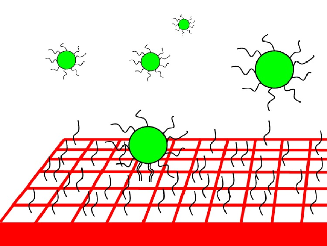
Figure 3.1: Graphical depiction of particles interacting with a flat, 2D substrate by multiple key-lock binding.

3.2 Model Description

We now present the model, where a single particle interacts with a flat two-dimensional surface by multiple key lock binding (see Fig. 3.1).  At each location on the surface there are $m$ key-lock bridges which may be open or closed, with a binding energy of $\epsilon$ for each key-lock pair.  Here we have neglected the variation in $\epsilon$.  In the case of the DNA-colloidal system mentioned in the introduction, the model parameter $\epsilon$ is related to the hybridization free energy of the DNA.  The resulting $m$-bridge free energy plays the role of an effective local potential for the particle [30]:

$$U(m) =-Tm\Delta$$ (3.1)

$$\Delta \equiv\log(1+\exp[\epsilon/T])$$ (3.2)

Generically, $m$ is a Poisson distributed random number $P_{m}=\overline{m}^{m}\exp(-\overline{m})/m!$ where $\overline{m}$ denotes the mean of the distribution.  The model parameter $\overline{m}$ is a collective property of the particle-surface system.  For example, consider the case of dendrimers functionalized with folic acid, which can be utilized for targeted, cell specific chemotherapy.  The folic acid on the dendrimer branch ends form key-lock bridges with folate receptors in the cell-membrane.  In this case $\overline{m}$ will depend on the distribution of keys (folic acids) on the dendrimer, and the surface coverage of locks (folate receptors) in the cell membrane.

At each location, the particle is attached to the surface by $m$ bridges.  To detach from the surface the particle must break all its connections, in which case it departs and diffuses away into solution.  Alternatively the particle can hop a distance $a$ to a new location characterized by a new value of the bridge number $m$.  By introducing the correlation length $a$, we have coarse-grained the particle motion by the distance after which the new value of the bridge number becomes statistically independent of the value at the previous location.  In the localized regime the particle remains close to its original location until departing.  In the diffusive regime the particle is able to fully explore the surface through a random walk by multiple breaking and reforming of bridges.

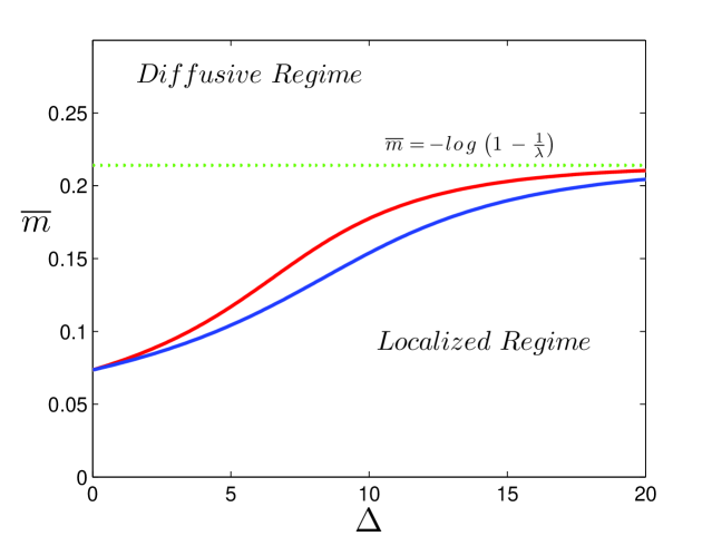
Figure 3.2: The crossover from the localized to the diffusive regime below the percolation threshold.  Estimates based on the characteristic cluster size (Eq. 3.3, red line) and confinement of the random walk (Eq. 3.4, blue line) give similar crossovers.  For large $\Delta$ the crossover condition is $\overline{m}=-\log\left(1-\frac{1}{\lambda}\right)$.  

3.3 Crossover from Localized to Diffusive Behavior

Naively one might expect the crossover between the two regimes to occur at the percolation threshold, where one first encounters an infinitely connected cluster of sites with $m>0$.  However, the crossover from the localized to diffusive regime occurs at smaller $\overline{m}$ than predicted by percolation theory.  If $p_{c}=1/2$ denotes the critical probability for site percolation on the triangular lattice, the percolation transition occurs at $\overline{m}=\log\left(2\right)$.  There are two alternative estimates for the crossover from the localized to the diffusive regime.  The first is to compare the average number of steps $n=\exp\left(\Delta\overline{m}\right)$ the particle takes before departing (see section 3.5) to the characteristic cluster size $s_{c}=1/\log(1/\lambda p)$ below the percolation threshold.  Here $\lambda=5.19$ is a numerical constant for the triangular lattice [78], and in the percolation language $p=1-\exp(-\overline{m})$ is the occupancy probability.  The crossover condition $n=s_{c}$ can be expressed as a function of $\overline{m}$.

$$\Delta=-\frac{1}{\overline{m}}\log\left[-\log\left\{\lambda\left(1-e^{-\overline{m}}\right)\right\}\right]$$ (3.3)

Alternatively, in the localized regime the particles’ random walk is confined by the characteristic cluster size.  Below percolation the radius of gyration of the cluster is $R_{s}\sim s^{\rho}$ with $\rho=0.641$ in two dimensions.  Comparing the radius of gyration of the cluster to the radius of gyration for the particles’ random walk, the crossover occurs at $n=\left(s_{c}\right)^{2\rho}$.

$$\Delta=-\frac{2\rho}{\overline{m}}\log\left[-\log\left\{\lambda\left(1-e^{-\overline{m}}\right)\right\}\right]$$ (3.4)

Since $2\rho$ differs from $1$ by less than $30\%$, both conditions give similar crossovers (see Fig. 3.2).  The saturation at $\overline{m}=-\log\left(1-\frac{1}{\lambda}\right)$ occurs for very large $\Delta$, as a result for binding energies of a few $T$ per bridge the crossover occurs at $\overline{m}\simeq 0.1$.

3.4 Localized Regime

In the percolation language, when the occupancy probability $p=1-\exp(-\overline{m})$ is small, particles are localized on finite clusters.  In this localized regime particles are able to fully explore the cluster to which they are attached before departing.  This thermalization of particles with finite clusters permits an equilibrium calculation of the cluster free energy $F=-T\log\langle Z\rangle$.  The departure rate is given by the Arrhenius relation $K=\frac{1}{\tau_{0}}\exp\left(F/T\right)$.  Here $\tau_{0}$ is a characteristic timescale for bridge formation.  The probability that the particle departs between $t$ and $t+dt$ is determined from the departure time distribution $\Phi(t)dt\simeq K\exp[-Kt]dt$.

To begin we calculate the partition function for the finite clusters.  The cluster is defined as $s$ connected sites on the lattice, all of which are characterized by $0<m<m^{\ast}$ bridges.  For Poisson distributed bridge numbers the partition function for the finite cluster is:

$$Z(m^{\ast},s)=\sum_{i=1}^{s}\sum_{m_{i}=1}^{m^{\ast}-1}\widetilde{P}_{m_{i}}\exp(\Delta m_{i})=\frac{s}{\exp(\overline{m})-1}(\exp(\overline{m}e^{\Delta})Q(\overline{m}e^{\Delta},m^{\ast})-1)$$ (3.5)

Because by definition the cluster does not contain sites with $m=0$ bridges we have renormalized the probability distribution $\widetilde{P}_{m}=P_{m}/(1-\exp(-\overline{m}))$ so that $\sum_{m=1}^{\infty}\widetilde{P}_{m}=1$.  Here $Q(x,m^{\ast})\equiv\Gamma(x,m^{\ast})/\Gamma(m^{\ast})=\exp(-x)\sum_{k=0}^{m^{\ast}-1}x^{k}/k!$ is the regularized upper incomplete $\Gamma$ function.  In the language of the statistics of extreme events, $m^{\ast}-1$ is the maximum ”expected” value of $m$ in a sample of $s$ independent realizations [79]. The point is that on finite clusters we should not expect to achieve arbitrarily large values of the bridge number.  Hence when averaging the partition function to obtain the cluster free energy one should only average over sites with $m<m^{\ast}$.  The distribution function for $m^{\ast}$ is obtained by noting that the probability that all $s$ values of $m$ are less than $m^{\ast}$ is $\left(\sum_{m=1}^{m^{\ast}-1}\widetilde{P}_{m}\right)^{s}=\left(\frac{\exp(\overline{m})Q(\overline{m},m^{\ast})-1}{\exp(\overline{m})-1}\right)^{s}$.  By differentiating this quantity with respect to $m^{\ast}$ we obtain the distribution function for the maximum expected value of $m$.

$$f_{s}(m^{\ast})=s\left(\frac{\exp(\overline{m})Q(\overline{m},m^{\ast})-1}{\exp(\overline{m})-1}\right)^{s-1}\widetilde{P}_{m^{\ast}}$$ (3.6)

The cluster size distribution below the percolation threshold is exponential [80] with characteristic cluster size $s_{c}=1/\log(1/\lambda p)$.

$$p_{s}(p)=\frac{1-\lambda p}{\lambda}\exp\left(-\frac{s}{s_{c}}\right)$$ (3.7)

The summation over $s$ can be performed analytically, which allows the result to be expressed as a single summation over $m^{\ast}$.

$$\langle Z\rangle=\sum_{m^{\ast}=2}^{\infty}\sum_{s=1}^{\infty}p_{s}(p)f_{s}(m^{\ast})Z(m^{\ast},s)=$$ (3.8)

$$\frac{\lambda(1-\lambda(1-\exp(-\overline{m})))}{\exp(\overline{m})-1}\sum_{m^{\ast}=2}^{\infty}\widetilde{P}_{m^{\ast}}(\exp(\overline{m}e^{\Delta})Q(\overline{m}e^{\Delta},m^{\ast})-1)\frac{1+y(m^{\ast})}{(1-y(m^{\ast}))^{3}}$$

$$y(m^{\ast})=\lambda(Q(\overline{m},m^{\ast})-\exp(-\overline{m}))$$ (3.9)

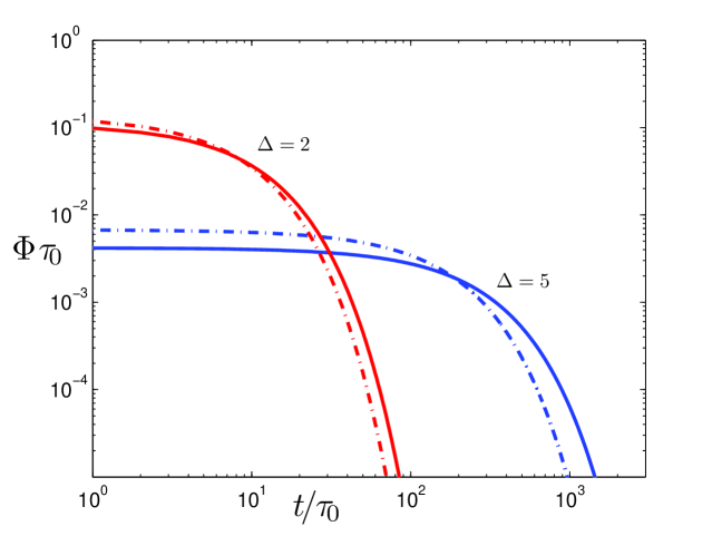
Figure 3.3: Departure time distribution function versus time in the localized regime with $\overline{m}=0.1$. The results of our calculation (solid lines) are compared to single exponential relaxation with departure rate $K=\frac{\exp(-\Delta)}{\tau_{0}}$ (dotted lines).

For fixed $\overline{m}$, as in the plot (see Fig. 3.3), changing $\Delta$ is directly related to a change in the average binding free energy.  Increasing $\Delta$ leads to a reduction in the rate of particle departure.

3.5 Diffusive Regime

The departure time distribution changes significantly in the diffusive regime.  In this regime the particle can explore the surface to find a more favorable connection site, which leads to a longer lifetime for the bound state.  This phenomenon is qualitatively similar to aging in glassy systems.  In these systems one finds that the response to an external field is time dependent [81].  In the magnetic analogy this leads to a time dependence of the magnetization.  Below the glass temperature, the longer one waits before applying the external magnetic field, the more time the system has to settle into deep energy wells, and the smaller the response.  In our case, the diffusive exploration of the particle allows it to find a deeper energy well, which leads to an increase in the bound state lifetime.

As a result, the departure time distribution must now reflect not only desorption, but also hopping to adjacent sites.  The hopping rate between neighboring sites $i$ and $j$ is given by an Arrhenius law $\kappa_{i\rightarrow j}=\frac{1}{\tau_{0}}\exp[-\Delta(m_{i}-m_{j})\theta(m_{i}-m_{j})]$, with $\theta(x)$ the Heaviside step function.  In a lattice model with coordination number $z$ the dwell time $\tau_{m}$ at a site with $m$ bridges is calculated by averaging over the hopping rates to the nearest neighbors (see Fig. 3.4).

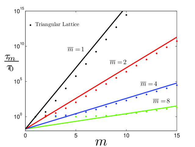
Figure 3.4: Comparison of the ensemble averaged dwell time in a lattice model (Eq. 3.10) to the effective Arrhenius approximation (Eq. 3.11).  In the plot the product $\Delta\overline{m}=4$ is held constant.

$$\tau_{m}=\left\langle\frac{1}{\frac{1}{z}\sum_{i=1}^{z}\kappa_{m\rightarrow i}}\right\rangle_{m_{1}...m_{z}}=z\sum_{m_{1}=1}^{\infty}\cdots\sum_{m_{z}=1}^{\infty}\widetilde{P}_{m_{1}}\cdots\widetilde{P}_{m_{z}}\frac{1}{\sum_{i=1}^{z}\kappa_{m\rightarrow i}}$$ (3.10)

Fortunately, this ensemble averaging procedure can be accurately approximated by an effective Arrhenius relation:

$$\tau_{m}=\tau_{0}\exp[\Delta(m-\overline{m})]$$ (3.11)

The validity of the approximation is most important for sites with $m\geq\overline{m}$ bridges, since the diffusive exploration allows the particle to quickly cascade into these deep energy wells.

The effective Arrhenius relation greatly simplifies the calculation, since so long as $\Delta\overline{m}$ is sufficiently large, the probability of the particle still being attached to the surface after an $n$ step random walk is $\left(1-K_{m}\tau_{m}\right)^{n-1}=[1-\exp(-\Delta\overline{m})]^{n-1}$.  Here $K_{m}=\frac{1}{\tau_{0}}\exp(-\Delta m)$ is the departure rate from a site with $m$ bridges.  Interestingly, in this approximation scheme the attachment probability is independent of the particular bridge numbers $\{m_{1},...,m_{n}\}$ realized during the walk.  Thus, the probability of departure $f_{n}$ after exactly $n$ steps is:

$$f_{n} =[\exp(\gamma)-1]\exp(-\gamma n)$$ (3.12)

$$\gamma \equiv-\log[1-\exp(-\Delta\overline{m})]$$ (3.13)

The average number of steps for the random walk is $\sum\nolimits_{n=1}^{\infty}nf_{n}=\exp(\Delta\overline{m})$.  To calculate the departure time distribution $\Phi(t)$ we use $f_{n}$ to average over the departure time distribution for walks with a given $n$, $\phi_{n}(t)$.

$$\Phi(t)=\sum\limits_{n=1}^{\infty}f_{n}\phi_{n}(t)$$ (3.14)

$$\phi_{n}(t)=\prod\limits_{j=1}^{n}\left(\sum_{m_{j}=1}^{\infty}\widetilde{P}_{m_{j}}\int_{0}^{\infty}dt_{j}\left(\frac{-dS_{m_{j}}(t_{j})}{dt_{j}}\right)\right)\delta\left(t-\sum_{k=1}^{n}t_{k}\right)$$ (3.15)

Here $S_{m}(t)$ is the survival probability at time $t$ for a site with $m$ bridges, used to determine the probability of departure between $t$ and $t+dt$.  If there was only one hopping pathway with rate $\kappa$, we would have $-\frac{dS}{dt}=\kappa\exp(-\kappa t)$.  The generalization accounts for the fact that the particle can hop to any of its $z$ neighbours, and the probability of departure is not simply exponential.

$$S_{m}(t)=\left(\sum\limits_{a=1}^{\infty}\widetilde{P}_{a}\exp\left[-t\kappa_{m\rightarrow a}\right]\right)^{z}$$ (3.16)

It is convenient to Fourier transform $\phi_{n}(t)$ so that one can sum the resulting geometric series for $\Phi(\omega)$.

$$\phi_{n}(\omega) =\int_{-\infty}^{\infty}\phi_{n}(t)\exp[-i\omega t]dt=X(\omega)^{n}$$ (3.17)

$$X(\omega) \equiv\sum_{m=1}^{\infty}\widetilde{P}_{m}\sum_{m_{1}=1}^{\infty}\cdots\sum_{m_{z}=1}^{\infty}\widetilde{P}_{m_{1}}\cdots\widetilde{P}_{m_{z}}\left(\frac{\sum\limits_{i=1}^{z}\kappa_{m\rightarrow m_{i}}}{\sum\limits_{i=1}^{z}\kappa_{m\rightarrow m_{i}}+i\omega}\right)$$ (3.18)

$$\Phi(\omega) =[\exp(\gamma)-1]\sum\limits_{n=1}^{\infty}\left[\exp(-\gamma)X(\omega)\right]^{n}=[\exp(\gamma)-1]\frac{X(\omega)}{\exp(\gamma)-X(\omega)}$$ (3.19)

To facilitate a simpler calculation, we employ a coarse-graining procedure to dispense with the tensor indices $\{m,m_{1},...,m_{z}\}$ in the definition of $X(\omega)$.  In the summation there are many terms for which the value of $\sum\limits_{i=1}^{z}\kappa_{m\rightarrow m_{i}}$ are equal, but with different weight factors $\widetilde{P}_{m}\widetilde{P}_{m_{1}}\cdots\widetilde{P}_{m_{z}}$.  To eliminate this degeneracy we introduce a smooth function $f(\kappa)$ normalized according to $\int f(\kappa)d\kappa=1$.

$$X(\omega)\simeq\int f(\kappa)\frac{\kappa}{\kappa+i\omega}d\kappa$$ (3.20)

The inverse Fourier transform is performed using the residue theorem to obtain the final result.  The contour integral is closed in the upper half plane, with all the poles on the imaginary axis at $\omega=iz$.

$$\Phi(t) =\frac{1}{2\pi}\int_{-\infty}^{\infty}\Phi(\omega)\exp[i\omega t]d\omega=\frac{[\exp(\gamma)-1]}{2\pi}2\pi i\sum_{r=1}^{\infty}res_{\omega=\omega_{r}}\left[\frac{\exp[i\omega t]X(\omega)}{\exp(\gamma)-X(\omega)}\right]$$ (3.21)

$$=[\exp(\gamma)-1]i\sum_{r=1}^{\infty}res_{\omega=\omega_{r}}\left[\frac{\exp[i\omega_{r}t]\left\{X(\omega_{r})+(\omega-\omega_{r})\left(\frac{dX}{d\omega}\right)_{\omega=\omega_{r}}+\cdots\right\}}{\exp(\gamma)-\left\{X(\omega_{r})+(\omega-\omega_{r})\left(\frac{dX}{d\omega}\right)_{\omega=\omega_{r}}+\cdots\right\}}\right]$$

$$=[\exp(\gamma)-1]i\sum_{r=1}^{\infty}\left[\frac{-\exp[i\omega_{r}t]X(\omega_{r})}{\left(\frac{dX}{d\omega}\right)_{\omega=\omega_{r}}}\right]$$

$$=\exp(\gamma)[\exp(\gamma)-1]\sum_{r=1}^{\infty}\frac{\exp(-z_{r}t)}{Y(z_{r})}$$

$$Y(z_{r}) \equiv\int f(\kappa)\frac{\kappa}{\left(\kappa-z_{r}\right)^{2}}d\kappa$$ (3.22)

Here $z_{r}$ labels the roots of the equation

$$\exp(\gamma)-X(iz)=0$$ (3.23)

The benefit of the coarse-graining is now more transparent, as the residues are all labeled by a single index $r$ as opposed to the tensor indices $\{m,m_{1},...,m_{z}\}$.

In Fig. 3.6 the departure time distribution is plotted in the diffusive regime.  The optimal regime for fast particle departure is to have a large number ($\overline{m}\sim 10$) of weakly bound key-lock bridges.  In this scenario the departure time distribution is accurately approximated as a single exponential, $\Phi(t)=K_{\overline{m}}\exp(-K_{\overline{m}}t)$.

We now discuss the behavior of the departure time distribution in several regimes of interest.  At fixed $\overline{m}$, for small $\Delta$ the behavior is non-universal.  The departure time distribution exhibits multi-stage behavior, where the initial departure and long time behavior may both take the shape of a power law, albeit with different exponents (see $\Delta=0.5$, $1$ curves in Fig. 3.5).

As the strength of the key-lock binding increases ($\Delta\gtrsim 1$) there is a crossover from non-universal behavior to universal power law behavior for the first several decades in time (see $\Delta=2$, $3$ curves in Fig. 3.5).

$$\Phi(t)\sim t^{-.7}$$ (3.24)

For $\Delta\gtrsim 3$ we enter the regime of multiexponential beating.  The initial departure behavior is well described as an exponential with initial departure rate $K_{\overline{m}}=\exp(-\Delta\overline{m})/\tau_{0}$ and characteristic timescale $1/\kappa^{\ast}\simeq 15\tau_{0}$.

$$\Phi(t)\simeq K_{\overline{m}}\exp(-\kappa^{\ast}t)$$ (3.25)

We attribute $\kappa^{\ast}$ to the diffusive cascade of particles from states with $\overline{m}$ bridges into more highly connected states.  Since this process involves particles finding a lower energy state, $\kappa^{\ast}$ does not depend on $\Delta$.  As indicated by the small departure probability, the binding is nearly irreversible in this regime (see $\Delta=5$, $7$ curves in Fig. 3.5).

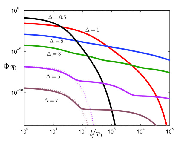
Figure 3.5: Departure time distribution function versus time with $\overline{m}=3$.  The dotted lines for $\Delta=5$ and $7$ show the exponential approximation $\Phi(t)=K_{\overline{m}}\exp(-\kappa^{\ast}t)$.  

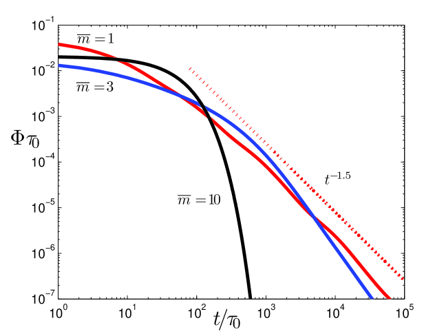
Figure 3.6: Departure time distribution function versus time as determined by Eq. 3.21 in the diffusive regime.  In the plot the average binding energy is held constant at $4T$. The theoretically determined departure time distribution can be compared to an experiment with DNA-grafted colloids which observed power law behavior with exponent $-1.5$.  

We also plot the departure time distribution relevant to the experimental situation where the average binding energy is held constant [30].

$$\frac{\Delta\overline{m}}{1-\exp(-\overline{m})}+\ln(1-\exp(-\overline{m}))=const.\$$ (3.26)

The optimal regime for fast departure is to have a large number ($\overline{m}\sim 10$) of weakly bound bridges (see Fig. 3.6).  In this fast departure regime the departure time distribution is well approximated as a single exponential, $\Phi(t)=K_{\overline{m}}\exp(-K_{\overline{m}}t)$ .

3.6 Diffusion

We now turn to discuss the statistics for the in-plane diffusion of the particle.  We first note that the in-plane trajectory of the particle subjected to a delta-correlated random potential remains statistically equivalent to an unbiased random walk.  As a result, the mean squared displacement for an $n$ step random walk remains $\left\langle r^{2}\right\rangle=na^{2}$.  As the particle explores the landscape it cascades into deeper energy wells, the hopping time increases, and the diffusion gets slower.  In the limit $n\rightarrow\infty$ the average hopping time can be determined from the equilibrium canonical distribution.  For Poisson distributed bridge numbers $m$, this corresponds to a finite renormalization of the diffusion coefficient $D^{\ast}$ with $D_{0}=a^{2}/4\tau_{0}$.

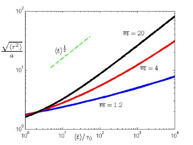
Figure 3.7: Root mean squared displacement vs. time with $\Delta\overline{m}=4$.  The curves are calculated from the parametric equations 3.29, 3.30.  

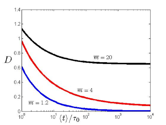
Figure 3.8: The dimensionless diffusion coefficient $D\equiv\frac{1}{4D_{0}}\frac{\partial\left\langle r^{2}\right\rangle}{\partial\left\langle t\right\rangle}$ plotted against time.  

$$\left\langle t\right\rangle=n\left\langle\tau_{m}\right\rangle=n\tau_{0}\exp\left(-\Delta\overline{m}\right)\sum_{m=1}^{\infty}\widetilde{P}_{m}\exp\left(\Delta m\right)=n\tau_{0}\frac{\exp\left(\overline{m}e^{\Delta}\right)-1}{\exp\left(\Delta\overline{m}\right)[\exp(\overline{m})-1]}$$ (3.27)

$$D^{\ast}\equiv\frac{1}{4}\frac{\partial\left\langle r^{2}\right\rangle}{\partial\left\langle t\right\rangle}=D_{0}\frac{\exp\left(\Delta\overline{m}\right)[\exp(\overline{m})-1]}{\exp\left(\overline{m}e^{\Delta}\right)-1}$$ (3.28)

This ”ergodic” behavior is only achieved after a very long time.  Generally, an $n$ step random walk cannot visit sites with arbitrarily large $m$.  In this transient regime one should only average over sites with $m<m^{\ast}$.  In the language of the statistics of extreme events, $m^{\ast}-1$ is the maximum ”expected” value of $m$ in a sample of $n$ independent realizations [79].  Even with this complication, the average diffusion time $\left\langle t\right\rangle$ and the mean squared displacement $\left\langle r^{2}\right\rangle$ can both be expressed in terms of $m^{\ast}$, which defines their relationship in parametric form.

$$\left\langle r^{2}\right\rangle=\frac{a^{2}}{P(\overline{m},m^{\ast})}$$ (3.29)

$$\left\langle t\right\rangle=\frac{\left\langle r^{2}\right\rangle}{D^{\ast}}\left(1-\frac{P(\overline{m}e^{\Delta},m^{\ast})}{1-\exp(-\overline{m}e^{\Delta})}\right)$$ (3.30)

Here $P(x,m^{\ast})\equiv\gamma(x,m^{\ast})/\Gamma(m^{\ast})=\exp(-x)\sum_{k=m^{\ast}}^{\infty}x^{k}/k!$ is the regularized lower incomplete $\Gamma$ function.  In the limit $m^{\ast}\rightarrow\infty$ we recover the renormalized diffusion relation $\left\langle t\right\rangle=\left\langle r^{2}\right\rangle/D^{\ast}$, although this occurs at very long, often unrealistic times.  In the transient regime we expect anomalous, subdiffusive behavior.  As indicated in Fig. 3.7, this subdiffusive behavior is typical for strong enough key-lock interactions.  Figure 3.8 is a plot of the dimensionless diffusion coefficient versus time.

By approximating the incomplete gamma functions, the transient behavior may be well described by a power law with a single free parameter $\beta\simeq 0.15$ (see Fig. 3.9).

$$\frac{\left\langle r^{2}\right\rangle^{\frac{1}{2}}}{a}\simeq\left(\frac{\left\langle t\right\rangle}{\tau_{0}}\right)^{\eta}$$ (3.31)

$$\eta=\frac{1}{2}-\frac{1+[\Delta-1]\exp(\Delta)}{2\Delta[\exp(\Delta)-1]-\frac{2}{\beta\overline{m}}\ln\left[1-\exp(-\beta\overline{m})\right]}$$ (3.32)

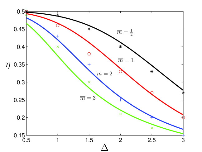
Figure 3.9: Comparison of the power law exponent determined numerically to Eq. 3.32 in the transient regime.  

There is an analogy between our results and dispersive transport in amorphous materials.  In these systems a length dependence of the effective mobility [82] can be interpreted within the context of the statistics of extreme events [79].  The time required for charge carriers to travel through the material depends on the dwell times spent at all of the trapping centers.  Since this transit time will be dominated by the dwell time of the deepest trapping center, one would like to know how the thickness of the material effects the distribution for the largest trapping depth.  The analogy to our result is made by replacing the material thickness with the number of steps in the random walk $n$, and replacing the distribution for the largest trap depth with the distribution for $m^{\ast}$, since the bridge number is related to energy by Eq. 3.1.

3.7 Connection to Experiments

We now would like to make a connection between our results and recent experiments with DNA-grafted colloids.  The departure time distribution can be compared to an experiment which determined the time-varying separation of two DNA-grafted colloids in an optical trap [26].  In the experimental setup, two particles are bound by DNA bridges, and after breaking all connections diffuse to the width of the optical trap.  Because the length of the DNA chains grafted on the particle is much shorter than the particle radius, surface curvature effects can be neglected.  The interaction resembles that of a particle interacting with a patch on a $2D$ substrate.  Experimentally the tail of the departure time distribution was observed to be a power law $\Phi(t)\sim t^{-1.5}$.  Qualitatively similar behavior is predicted by the theory with $\overline{m}\sim 1$ and average binding free energy of several $T$ (see $\overline{m}=1$ curve in Fig. 3.6).

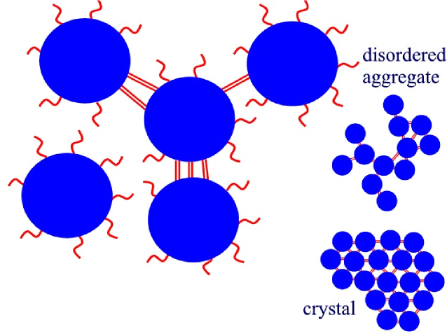
Figure 3.10: Graphical depiction of key-lock binding between nanoparticles functionalized with complementary ssDNA.  The resulting structures can be disordered, fractal-like aggregates, or crystalline.  

In addition, our work provides insight into the slow crystallization dynamics of key-lock binding particles (see Fig. 3.10).  In [1], $1\mu m$ diameter particles grafted with ssDNA formed reversible, disordered aggregates.  The average number of key-lock bridges between particles was $\overline{m}\sim 2$.  The authors of [26] observed random hexagonal close packed crystals by further reducing the surface density of DNA strands on the particles.  The crystallization process requires that particles rapidly detach and reattach at the desired lattice location.  In the localized regime particle desorption is the relevant process.

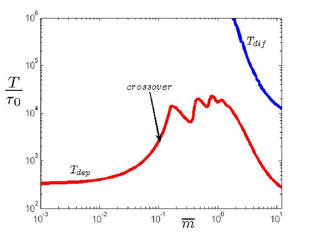
Figure 3.11: Plot of the characteristic times $T_{dep}$ and $T_{dif}$ versus $\overline{m}$ at constant binding energy ($const=4$ in Eq. 3.34).  

In the diffusive regime surface diffusion also plays a role in the rearrangement of particles into the desired crystalline structure.  To determine which process is more important for particle rearrangement, we can compare the departure time with the time required for a particle to diffusively explore the surface of a particle to which it is bound.  The time $T_{dep}$ required for $90\%$ of the particles to depart is:

$$0.1=\int_{T_{dep}}^{\infty}\Phi(t)dt$$ (3.33)

To estimate the time required for diffusive rearrangement $T_{dif}$ we use the parametric equations 3.29, 3.30.  In [1] particles of radius $R=.5\mu m$ were grafted with DNA chains of length $l\sim 20nm$.  Assuming the correlation length $a\sim l$ we have $\frac{\left\langle r^{2}\right\rangle}{a^{2}}\sim\left(\frac{\pi R}{l}\right)^{2}\simeq 10^{3}$.  Figure 3.11 shows a comparison of $T_{dif}$ and $T_{dep}$ at constant binding free energy.

$$\frac{\Delta\overline{m}}{1-\exp(-\overline{m})}+\log(1-\exp(-\overline{m}))=const$$ (3.34)

This expression for the binding energy takes into account the entropy reduction associated with the non-ergodic degrees of freedom.  For a detailed discussion of this topic see reference [30].  Since $T_{dif}>T_{dep}$, colloidal desorption and reattachment is the dominant mechanism by which particles rearrange.

As the figure indicates, the optimal regime of fast departure is to have a large number ($\overline{m}\gtrsim 10$) of weakly bound key-lock bridges.  We predict a localized regime below the crossover where particle departure is relatively fast.  Just beyond the crossover there is a relative maximum in $T_{dep}$ before it decreases at large $\overline{m}$.  The increase in departure time at the onset of diffusive behavior is indicative of a regime where the system ages.  In this regime the interplay of diffusion an desorption leads to longer bound state lifetimes, and an increase in the departure time.

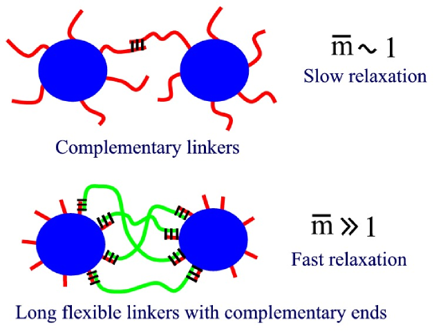
Figure 3.12: Graphical depiction comparing recent experiments with DNA-grafted colloids to a future implementation with long flexible linkers.  Increasing the number of key-lock bridges between particle pairs potentially decreases the time required for crystallization.  

We now turn to the question of designing a future experiment which will facilitate fast particle departure and hence colloidal crystallization.  The essential goal is to increase the average number of key-lock bridges between particle pairs.  Increasing the surface density of DNA strands alone results in the formation of a brush, which decreases the effective cross section for the interaction between complementary DNA.  Instead we propose the introduction of long, flexible DNA linkers between particles with a high coverage of short ssDNA (see Fig. 3.12).  This system has the potential to realize more key-lock bridges between particle pairs as compared to previous experiments, and therefore substantially reduce the time required for crystallization.

3.8 Summary

In this chapter we studied the dynamics of particles which interact through the reversible formation of multiple key-lock bridges.  Well before the percolation threshold is reached there is a crossover from a localized regime to a diffusive regime.  In the localized regime the particles remain close to their original attachment site until departing.  In this regime particles are attached to finite clusters, and the system exhibits an exponential distribution of departure times.  Once the radius of gyration of the cluster exceeds the characteristic radius for the particles’ random walk, the finite clusters behave effectively as infinite clusters.  Diffusion allows the particles to cascade into deeper energy wells, which leads to a decrease in hopping rate.  The diffusion slows and the bound state lifetime increases, a phenomenon qualitatively similar to aging in glassy systems.  In the diffusive regime we discussed the statistics for the particles’ in-plane diffusion.  Weak key-lock interactions give rise to a finite renormalization of the diffusion coefficient.  However, as the strength of the interaction increases (larger $\Delta$), the system exhibits anomalous, subdiffusive behavior.  This situation is analogous to dispersive transport in disordered semiconductors.  We then made the connection between our calculation of the departure time distribution and recent experiments with DNA-coated colloids.  The findings indicate that the optimal regime for colloidal crystallization is to have a large number of weakly bound key-lock bridges.  A modified experimental setup was proposed which has the potential to realize this regime of fast particle departure.

Chapter 4 Self-Assembly of DNA-Coded Clusters

4.1 Motivation and Problem Description

Over the past decade, a number of proposals have identified potential applications of DNA for self-assembly of micro- and nanostructures [18], [17], [46], [47], [48].  Among these proposals, one common theme is finding a way to utilize the high degree of selectivity present in DNA-mediated interactions.  An exciting and potentially promising application of these ideas is to use DNA-mediated interactions to programmable self-assemble nanoparticle structures [25], [15], [45], [44].  Generically, these schemes utilize colloidal particles functionalized with specially designed ssDNA (markers), whose sequence defines the particle type.  Selective, type-dependent interactions can then be introduced either by making the markers complementary to each other, or by using linker-DNA chains whose ends are complementary to particular maker sequences.  Independent of these studies, there are numerous proposals to make sophisticated nano-blocks which can be used for hierarchical self-assembly. One recent advance in the self-assembly of anisotropic clusters is the work of Manoharan et. al [3].  They devised a scheme to produce stable clusters of $n$ polystyrene microspheres.  The clusters were assembled in a colloidal system consisting of evaporating oil droplets suspended in water, with the microspheres attached to the droplet interface.  The resulting clusters, unique for each $n$, are optimal in the sense that they minimize the second moment of the mass distribution $M_{2}=\sum_{i=1}^{n}(\mathbf{r}_{i}-\mathbf{r}_{cm})^{2}$.

In this chapter [61], we present a theoretical discussion of a method which essentially merges the two approaches. We propose to utilize DNA to self-assemble colloidal clusters, somewhat similar to those in Ref. [3].  An important new aspect of the scheme is that the clusters are ”decorated”: each particle in the resulting cluster is distinguished by a unique DNA marker sequence. As a result, the clusters have additional degrees of freedom associated with particle permutation, and potentially may have more selective and sophisticated inter-cluster interactions essential for hierarchic self-assembly.  In addition, the formation of such clusters would be an important step towards programmable self-assembly of micro- and nanostructures of an arbitrary shape, as suggested in Ref. [65].

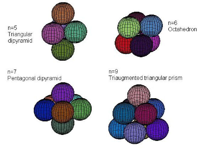
Figure 4.1: The minimal second moment clusters for $n=5,6,7,$ and $9$.  Pictures of all the clusters from $n=4$ to $15$ are available in [3].

Table 4.1: Minimal Second Moment Clusters

$n$	Polyhedra Name	Schönflies Point Group
$4$	Tetrahedron	$T_{d}$
$5$	Triangular dipyramid	$D_{3h}$
$6$	Octahedron	$O_{h}$
$7$	Pentagonal dipyramid	$D_{5h}$
$8$	Snub disphenoid	$D_{2d}$
$9$	Triaugmented triangular prism	$D_{3h}$
$10$	Gyroelongated square dipyramid	$D_{4d}$
$11$	(non-convex)	$C_{S}$

We begin with octopus-like particles functionalized with dsDNA, with each strand terminated by a short ssDNA marker sequence.  We assume that each particle $i$ has a unique code, i.e. the maker sequence $s_{i}$ of ssDNA attached to it.  We then introduce anchor DNA to the system, ssDNA with sequence $\overline{s}_{A}\overline{s}_{B}...\overline{s}_{n}$, with $\overline{s}_{i}$ the sequence complementary to the marker sequence $s_{i}$.  The anchor is designed to hybridize with one particle of each type.  Consider a cluster of $n$ particles attached to a single anchor.

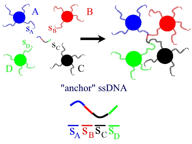
Figure 4.2: Schematic representation of the method for constructing decorated colloidal clusters using ssDNA ”anchors”.  

If we treat the DNA which link the particles to the anchor as Gaussian chains, there is an entropic contribution to the cluster free energy which can be expressed in terms of the particle configuration $\{\mathbf{r}_{1},...,\mathbf{r}_{n}\}$ as follows.  Here $R_{g}$ is the radius of gyration of the octopus-like DNA arms.

$$F=\frac{3T}{2R_{g}^{2}}\sum_{i=1}^{n}(\mathbf{r}_{i}-\mathbf{r}_{anchor})^{2}$$ (4.1)

This approximation of the DNA arms as Gaussian chains is acceptable provided their length $L$ exceeds the persistence length $l_{p}\simeq 50$ $nm$ and the probability of self-crossing is small [55].  The physical mechanism which determines the final particle configuration in our system is quite different from the capillary forces of Manoharan et al.  However, because the functional form of the free energy is equivalent to the second moment of the mass distribution, the ground state of the cluster should correspond to the same optimal configuration.

4.2 Equilibrium Treatment

Consider a system with $n$ particle species and an anchor of type $\overline{s}_{A}\overline{s}_{B}...\overline{s}_{n}$.  The clusters we would like to build contain $n$ distinct particles (each particle in the cluster carries a different DNA marker sequence) attached to a single anchor.  Let $C_{n}$ denote the molar concentration of the desired one anchor cluster.  Because there are many DNA attached to each particle, multiple anchor structures can also form.  The question is whether the experiment can be performed in a regime where the desired one anchor structure dominates, avoiding gelation.

We consider the stability of type $C_{n}$ with respect to alternative two anchor structures.  To do so we determine the concentration $C_{n+1}$ of $n+1$ particle structures which are maximally connected, but do not have a $1:1:\cdots:1$ composition.  In particular, these structures contain more than one particle of each type, which could cause problems in our self-assembly scheme [65].  There are also $n$ particle structures $\widetilde{C}_{n}$ with the correct composition, but which contain two anchors.  We would like to avoid the formation of these structures as well, as their presence decreases the overall yield of type $C_{n}$.  Figure 4.3 enumerates the various structures for an $n=3$ species system.  If the experiment can be performed as hoped, we will find a regime where the ratios $\frac{C_{n+1}}{C_{n}}$ and $\frac{\widetilde{C}_{n}}{C_{n}}$ are small.  To this end, the equilibrium concentrations $C_{n}$, $C_{n+1}$, and $\widetilde{C}_{n}$ are determined by equilibrating the chemical potential of the clusters with their constituents.

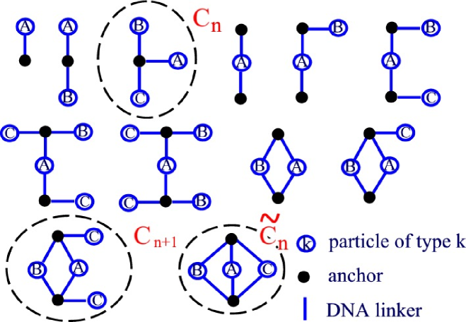
Figure 4.3: The topologically distinct one and two anchor structures for an anchor ssDNA with sequence $\overline{s}_{A}\overline{s}_{B}\overline{s}_{C}$.  Different structure varieites may be obtained by relabeling the particle indices subject to the constraint that no more than one particle of each type is attached to a given anchor.  

First we determine the molar concentration $C_{n}$ of the desired one anchor structure, composed of one anchor and $n$ particles.  Let $c_{i}$ denote the molar concentration of species $i$, and $c_{a}$ the molar anchor concentration.  Here $c_{o}=1M$ is a reference concentration.

$$T\log\left(\frac{c_{a}\mathop{\textstyle\prod}\limits_{i=1}^{n}c_{i}}{c_{o}^{n+1}}\right)=T\log\left(\frac{C_{n}}{c_{o}}\right)+\epsilon_{n}$$ (4.2)

$$\epsilon_{n}=\mathop{\textstyle\sum}\limits_{i=1}^{n}\Delta G_{i}-T\log\left(N^{n}v^{n}c_{o}^{n}\right)$$ (4.3)

$$C_{n}=N^{n}v^{n}c_{a}\mathop{\textstyle\prod}\limits_{i=1}^{n}c_{i}\exp\left[-\frac{\Delta G_{i}}{T}\right]$$ (4.4)

Here $\epsilon_{n}$ is the binding free energy of the cluster, which has a contribution from the hybridization free energy $\Delta G_{i}$ associated with attaching particle $i$ to the anchor, and an entropic contribution from the number of ways to construct the cluster(since each particle has $N$ hybridizable DNA arms).  In addition we must take into account the entropy for the internal degrees of freedom in the structure stemming from the flexibility of the DNA attachments to the anchor.  In the Gaussian approximation, neglecting the excluded volume between particles this localization volume $v\sim R_{g}^{3}$ can be calculated exactly.

$$F(\mathbf{r}_{1},...,\mathbf{r}_{n}) = \frac{3T}{2R_{g}^{2}}\sum_{i=1}^{n}r_{i}^{2}$$ (4.5)

$$v^{n} = \int d^{3}r_{1}...d^{3}r_{n}\exp\left[-\frac{F(\mathbf{r}_{1},...,\mathbf{r}_{n})}{T}\right]$$ (4.6)

$$v = R_{g}^{3}\left(\frac{2\pi}{3}\right)^{\frac{3}{2}}$$ (4.7)

We now consider the competing two anchor structure $C_{n+1}$.  To determine the equilibrium concentration it is instructive to consider the reaction in which two clusters of type $C_{n}$ combine to form a single cluster of type $C_{n+1}$ and release $n-1$ particles into solution.  Since there are many DNA attached to each particle, in what follows we omit factors of $\frac{N-1}{N}$.

$$2T\log\left(\frac{C_{n}}{c_{o}}\right)+2\epsilon_{n}=T\log\left(\frac{C_{n+1}}{c_{o}}\right)+\epsilon_{n+1}+\mathop{\textstyle\sum}\limits_{i=1}^{n-1}T\log\left(\frac{c_{i}}{c_{o}}\right)$$ (4.8)

$$\epsilon_{n+1}=2\mathop{\textstyle\sum}\limits_{i=1}^{n}\Delta G_{i}-T\log\left(N^{n+1}(N-1)^{n-1}v_{2}^{n+2}c_{o}^{n+2}\right)$$ (4.9)

$$C_{n+1}=\frac{v_{2}^{n+2}}{v^{2n}}\frac{C_{n}^{2}}{\mathop{\textstyle\prod}\limits_{i=1}^{n-1}c_{i}}$$ (4.10)

The localization volume $v_{2}$ can be calculated in a similar fashion, fixing one particle at the origin and integrating over the $n$ remaining particle positions $\{\mathbf{r}_{1},...,\mathbf{r}_{n}\}$ and the position of the two anchors $\mathbf{r}_{a1}$ and $\mathbf{r}_{a2}$.  We make use of the following formula for multivariate Gaussian integrals.

$$\mathop{\displaystyle\idotsint}_{-\infty}^{\infty}\exp\left[-\frac{q^{T}Mq}{2}\right]dq_{1}...dq_{3(n+2)}=\frac{\left(2\pi\right)^{\frac{3(n+2)}{2}}}{\sqrt{\det(M)}}$$ (4.11)

  

$$F(\mathbf{r}_{1},...,\mathbf{r}_{n,}\mathbf{r}_{a1},\mathbf{r}_{a2})=\frac{3T}{2R_{g}^{2}}[r_{a1}^{2}+(\mathbf{r}_{n}-\mathbf{r}_{a2})^{2}+\mathop{\textstyle\sum}\limits_{i=1}^{n-1}\left\{(\mathbf{r}_{i}-\mathbf{r}_{a1})^{2}+(\mathbf{r}_{a2}-\mathbf{r}_{i})^{2}\right\}]$$ (4.12)

$$v_{2}^{n+2}=\int d^{3}r_{1}...d^{3}r_{n}d^{3}r_{a1}d^{3}r_{a2}\exp\left[-\frac{F}{T}\right]$$ (4.13)

$$v_{2}=R_{g}^{3}\left(\frac{2\pi}{3}\right)^{\frac{3}{2}}n^{\frac{-3}{n+2}}2^{\frac{-3(n-1)}{2(n+2)}}=n^{\frac{-3}{n+2}}2^{\frac{-3(n-1)}{2(n+2)}}v$$ (4.14)

Similarly one can obtain the cluster concentration for the two anchor structure $\widetilde{C}_{n}$.  The localization volume $v_{3}$ can be calculated in a similar fashion to $v_{2}$.

$$v_{3}=R_{g}^{3}\left(\frac{2\pi}{3}\right)^{\frac{3}{2}}n^{\frac{-3}{2(n+1)}}2^{\frac{-3n}{2(n+1)}}=n^{\frac{-3}{2(n+1)}}2^{\frac{-3n}{2(n+1)}}v$$ (4.15)

We consider the symmetrical case $\Delta G_{i}=\Delta G$ and equal initial particle concentrations $c_{i}^{(o)}=c^{(o)}$ for all species $i$.  In this case we have $c_{A}=c_{B}=...=c_{n}\equiv c$.  We can express the concentration of the competing two anchor structures $C_{n+1}$ and $\widetilde{C}_{n}$ in terms of the concentration of the desired one anchor cluster $C_{n}$.  Since there are many DNA attached to each particle, we omit factors of $\frac{N-1}{N}$.

$$C_{n}=c_{a}\left(Nvc\ \exp\left[-\frac{\Delta G}{k_{B}T}\right]\right)^{n}$$ (4.16)

$$C_{n+1}\simeq\frac{v_{2}^{n+2}}{v^{2n}}\frac{C_{n}^{2}}{c^{n-1}}$$ (4.17)

$$\widetilde{C}_{n}\simeq\frac{v_{3}^{n+1}}{v^{2n}}\frac{C_{n}^{2}}{c^{n}}$$ (4.18)

The concentration of free anchors $c_{a}$ can be determined from the equation for anchor conservation.

$$c_{a}^{(o)}=c_{a}+C_{n}+2\widetilde{C}_{n}+2nC_{n+1}$$ (4.19)

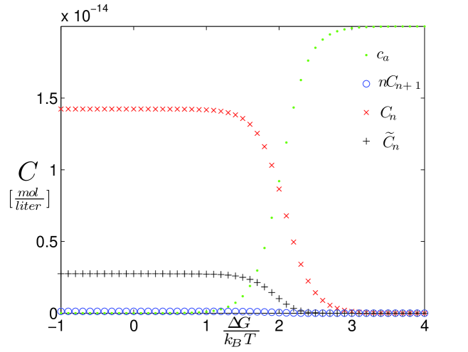
Figure 4.4: The molar concentrations $c_{a}$, $C_{n}$, $nC_{n+1}$, and $\widetilde{C}_{n}$ in the symmetrical case for a system with $n=5$ particle species.   The total particle volume fraction $n\phi\approx.25$ and $\frac{c_{a}^{(o)}}{c^{(o)}}=10^{-3}$.  

We are interested in the low temperature regime where there are no free anchors in solution.  We determine the saturation values for the ratios of interest by noting that the Boltzmann factor $\delta\equiv\exp\left[-\frac{\Delta G}{T}\right]\gg 1$ in this regime.

$$\frac{C_{n+1}}{C_{n}}\simeq\frac{n^{-3}2^{-3n+\frac{9}{2}}}{(R_{g}^{3}c^{(o)})^{n-2}}\frac{c_{a}^{(o)}}{c^{(o)}}+O\left(\frac{1}{\delta^{n}}\right)$$ (4.20)

$$\frac{\widetilde{C}_{n}}{C_{n}}\simeq\frac{n^{-3/2}2^{-3n+\frac{3}{2}}}{(R_{g}^{3}c^{(o)})^{n-1}}\frac{c_{a}^{(o)}}{c^{(o)}}+O\left(\frac{1}{\delta^{n}}\right)$$ (4.21)

Since $\frac{C_{n+1}}{\widetilde{C}_{n}}\ll 1$, eq. 4.21 provides the experimental constraint for suppressing the two anchor structures.  Taking the radius of the hard spheres $R\sim R_{g}$, it can be interpreted as a criterion for choosing the initial anchor concentration $c_{a}^{(o)}$ for an $n$ species system with $\phi=\frac{4\pi}{3}R_{g}^{3}c^{(o)}$ the particle volume fraction for an individual species.

$$\frac{c_{a}^{(o)}}{c^{(o)}}\lesssim n^{\frac{3}{2}}(2\phi)^{n-1}$$ (4.22)

The condition gives the maximum anchor concentration for the two anchor structures to be suppressed.  Since $\phi\leq\frac{1}{n}$ the theoretical limits are $\frac{c_{a}^{(o)}}{c^{(o)}}\lesssim 1$, $.29$, $.06$, and $.01$ for $n=4$, $5$, $6$, and $7$ respectively.  In figure 4.4 we plot the solution for the concentrations.  There is a large temperature regime($\frac{\Delta G}{k_{B}T}\lesssim 2$) where the two anchor structures are suppressed in favor of the desired one anchor structures.

4.3 Irreversible Binding

In the previous section we performed an equilibrium calculation to determine the yield of the cluster $C_{n}$ [61].  The results of that study indicated that the concentration of anchors must be kept very small to prevent the aggregation of larger clusters (see Eq. 4.22).  From an experimental perspective this result is somewhat disappointing, since the overall yield of the cluster $C_{n}$ is proportional to the anchor concentration.  The situation is considerably improved in the regime of irreversible binding of particles to anchors.  In what follows we present a calculation for the yield of the desired one anchor cluster far from equilibrium.  To distinguish between the results of the previous section and the regime of irreversible binding we will change the notation slightly.  This change reflects the fact that the role of the DNA anchor could also be played by a patchy colloidal particle as discussed below.  Henceforth we will refer to the DNA anchors as DNA scaffolds.  In the new notation the desired one anchor cluster $C_{n}$ is called the star cluster.

The plan for this section is the following.  The goal is to maximize the yield for the star cluster.  We analytically calculate the yield of the star cluster in the regime of irreversible binding.  The analytical results are compared to the numerical results for the full aggregation equations.  From an experimental perspective, the most important result is the determination of an optimal concentration ratio for experiments (see Eq. 4.30).  To conclude we discuss the experimental feasibility of the self-assembly proposal.

The basic idea behind the procedure is as follows (see Fig. 4.5).  Particles are functionalized with single-stranded DNA (ssDNA) markers which determine the particle color.  There may be many DNA attached to each particle, but on any given particle the marker sequence is identical.  One then introduces DNA scaffolds to the system.  The scaffold is a structure with $n$ ssDNA markers, each marker complementary to one of the particle colors.  Hybridization of the ssDNA markers on the particles to those on the scaffold results in the formation of colored particle clusters.  Because there are many DNA attached to each particle, clusters can form which contain more than one scaffold.  The essential goal of the procedure is to maximize the concentration of a particular type of cluster which we denote the star cluster.  The star cluster contains one and only one scaffold to which $n$ particles are attached, each particle having a distinct color.

We should note that the role of the scaffold could also be played by a patchy particle ([83],[84],[85]).  For example, these patches are regions on the particle surface where one can graft ssDNA markers.  In this case there may be several DNA connections between a patch and colored particle.  Our conclusions will still be valid, provided the patch size is chosen so that a patch interacts with at most one particle.

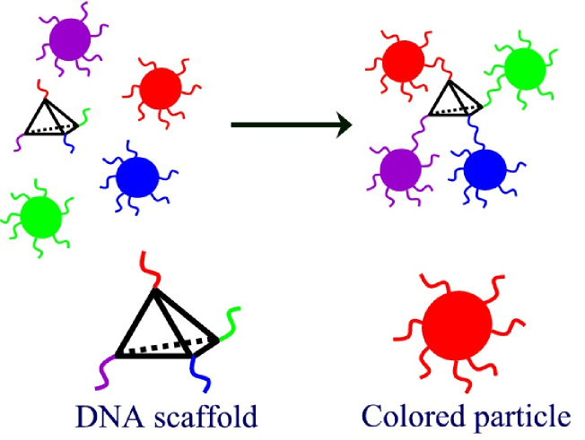
Figure 4.5: A graphical depiction of the scheme for self-assembling star clusters using DNA scaffolds.  In the diagram (not drawn to scale) the scaffold funcionality $n=4$.  

To understand the basic physics behind the aggregation process we consider the mobility mismatch between the particles and the scaffolds.  In solution, a particle with radius $R\simeq 1\mu m$ has a diffusion coefficient given by the Stokes-Einstein relation $D=k_{B}T/6\pi\eta R$.  On the other hand, the size of the scaffold $a\simeq 10nm$.  As a result the scaffolds diffuse $R/a\simeq 100$ times faster than the particles.  To first approximation the resulting aggregation is a two stage process.  In the first stage the particles recruit different numbers of scaffolds via the fast scaffold diffusion and subsequent DNA hybridization.  Since we consider the regime of strong binding where these bonds are irreversible, the result is a Poisson distribution over the concentration of particles with $m$ scaffolds attached.  Let $C_{i}$ denote the concentration of particles with color $i$, and $c$ denote the total concentration of scaffolds.  The total particle concentration $C_{tot}=\sum_{i=1}^{n}C_{i}$.  The concentration $C_{i}^{(m)}$ of particles of color $i$ with $m$ scaffolds attached is

$$C_{i}^{(m)} = C_{i}\frac{p^{m}\exp(-p)}{m!}$$ (4.23)

$$p = \frac{c}{C_{tot}}$$ (4.24)

In the second stage there are no free scaffolds left in solution, and these particles decorated with scaffolds aggregate to form the final clusters.  The seed to build a star cluster is a particle of any color with exactly one scaffold attached.  This seed must aggregate with $n-1$ particles of different colors, each of which has no scaffolds.  We now calculate the concentration of the star cluster $C_{\ast}$.  The yield of the desired star cluster is quantified in terms of the star mass fraction $M_{\ast}=(nC_{\ast})/C_{tot}$.

$$M_{\ast}=\frac{n}{C_{tot}}\sum\limits_{i=1}^{n}C_{i}^{(1)}\prod\limits_{\begin{subarray}{c}j=1\\ j\neq i\end{subarray}}^{n}\frac{C_{j}^{(0)}}{C_{j}}=x\exp(-x)$$ (4.25)

Here $x=np$ is the scaffold functionality $n$ multiplied by the concentration ratio $p$.  By choosing $p=1/n$ the mass fraction attains a maximum of $\exp(-1)\simeq 0.37!$  This result indicates that by selecting the appropriate scaffold concentration, in the nonequilibrium regime up to $37\%$ of the particles will aggregate to form star clusters.  This is a significant improvement over the situation in the equilibrium regime.

This treatment of the problem captures the physics of star cluster formation, but it does not account for the loss of star clusters due to aggregation.  In particular, as long as there are scaffolds with markers available for hybridization, when these scaffolds encounter a star cluster they can aggregate to form a larger cluster.  We now estimate how this aggregation effects the final concentration of star clusters.

Consider the beginning of the second stage in our aggregation process.  There are no longer any free scaffolds in solution, but a scaffold can have up to $n-1$ DNA markers still available for hybridization.  We would like to determine how the star cluster mass fraction $M_{\ast}(y)$ changes as a function of the fraction of saturated scaffolds $y$.  Here a saturated scaffold has particles hybridized to all $n$ of its DNA markers, and is therefore unreactive.  If $s$ is the expectation that a slot on the scaffold is filled, then the fraction of saturated scaffolds is $y=s^{n-1}$.  The average number of open slots on a scaffold is $(n-1)(1-s)$.  Consider filling an open slot on the scaffold.  The probability that the particle which filled the slot was part of a star cluster is $M_{\ast}(y)$.  The average rate $r(y)$ at which star clusters are lost to aggregation is then

$$r(y)=-M_{\ast}(y)\frac{d}{dy}\left[(n-1)(1-s)\right]=M_{\ast}(y)y^{-\alpha}\text{.}$$ (4.26)

Here the exponent $\alpha=(n-2)/(n-1)$.  We can then construct a differential equation for $M_{\ast}$ taking into account this loss due to aggregation.

$$\frac{dM_{\ast}}{dy}=\frac{dM_{\ast}^{(o)}}{dy}-xr(y)$$ (4.27)

In the absence of this loss term the result of the calculation should recover our previous result Eq. 4.25.  This zeroth order approximation is just $M_{\ast}^{(o)}(y)=xy\exp(-xy)$ which gives the correct star cluster concentration once all of the scaffolds are saturated ($y=1$).  To simplify the analysis a bit we take $\alpha=1$ which is an excellent approximation in the limit of large scaffold functionality $n$.  This is an inhomogeneous first order differential equation which can be solved by introducing an integrating factor $u(y)=y^{x}$.   The initial condition which must be satisfied is $M_{\ast}(0)=0$.  We are interested in the final star mass fraction $M_{\ast}$, which is $M_{\ast}(y=1)$.  The result is

$$M_{\ast} = x\sum_{k=0}^{\infty}\frac{(-x)^{k}}{k!}\left[\frac{1}{x+k+1}-\frac{x}{x+k+2}\right]$$

$$= x\exp(-x)+x^{2}E_{-x}(x)-x^{1-x}\Gamma(1+x)$$

Here $\Gamma(x)$ is the gamma function and $E_{\nu}(x)=\int\limits_{1}^{\infty}t^{-\nu}\exp(-xt)dt$ is the exponential integral of order $\nu$.

We can perform a similar type of analysis in the case when there is only one particle color.  In this case the $n$ ssDNA markers on the scaffold all have identical sequences complementary to this color.  It turns out that the result for the mass fraction is the same.  Because the mass fraction is the same in both cases, we can gain insight into the behavior of the system with many colors by analyzing the much simpler one color system.  To test our predictions, we numerically solved a system of differential equations which models the irreversible aggregation between particles (one color) and scaffolds.

$$\frac{dC_{IJ}}{dt}=\frac{1}{2}\sum\limits_{\begin{subarray}{c}i+i^{\prime}=I\\ j+j^{\prime}=J\end{subarray}}K_{iji^{\prime}j^{\prime}}C_{ij}C_{i^{\prime}j^{\prime}}-C_{IJ}\sum\limits_{i,j}K_{ijIJ}C_{ij}$$ (4.29)

This equation is the Smoluchowski coagulation equation [86] adapted to our system.  $C_{ij}$ is the concentration of the cluster with $i$ scaffolds and $j$ particles. $\ K_{iji^{\prime}j^{\prime}}$ is the rate constant for the irreversible reaction $C_{ij}+C_{i^{\prime}j^{\prime}}\rightarrow C_{i+i^{\prime}j+j^{\prime}}$.  We assume that the rates are diffusion limited in which case we can estimate the rate for any pair of clusters by $K_{iji^{\prime}j^{\prime}}=4\pi D_{s}R_{l}$.  The larger cluster with hydrodynamic radius $R_{l}\sim n_{l}^{1/3}$ plays the role of a sink.  Here $n_{l}$ is the number of particles in the larger cluster and $D_{s}=k_{B}T/6\pi\eta R_{s}$ is the diffusion constant for the smaller cluster.  To simply matters we only consider tree like structures, i.e. we do not consider the formation of clusters with internal loops.  We have truncated the set of equations by considering clusters with a maximum of $10$ scaffolds.

By solving these equations we can determine the concentration of stars $C_{\ast}=C_{1n}$ in this notation and test the validity of our two stage ansatz.  As indicated in Fig. 4.6, the result of our analytical calculation matches the results of the full numerical calculation up to an overall normalization factor of order unity.  Several points are in order.

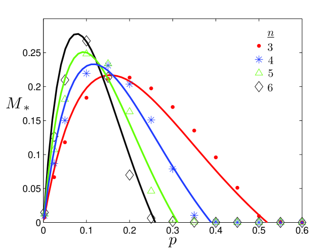
Figure 4.6: The mass fraction $M_{\ast}$ as a function of $p$ for scaffolds with functionality $n=3$ (red), $4$ (blue), $5$ (green), and $6$ (black).  The results determined numerically from the full solution of the Smoluchowski coagulation equation (markers) can be compared to results of the anlaytical calculation (lines) Eq. 4.3.  The resulting agreement is good up to an overall normalization factor $\gamma_{n}$ in the range $1.2$ to $1.5$ which normalizes the analytical curves.  

The optimal concentration ratio $p$ for experiments is easily determined from $\frac{dM_{\ast}}{dx}=0$.  The result is $x_{\max}\simeq 0.47$.  For scaffolds of functionality $n$ the concentration ratio should be chosen as:

$$p=\frac{0.47}{n}\text{.}$$ (4.30)

Note that the maximum attainable star cluster yield $M_{\ast}(x_{\max})\simeq 1/4$ does not decrease with increasing $n$.  In fact, the numerical results predict a slight increase in star cluster yield for larger $n$.  Solving the aggregation equations becomes computationally expensive, but it can still be done by reducing the maximum number of scaffolds in a cluster.  For example, considering clusters with up to $5$ scaffolds for $n=10$ gives $M_{\ast}(x_{\max})\simeq 0.3$.  These results are important from the perspective of experimental feasibility for the self-assembly method.  This is to be contrasted with the earlier equilibrium treatment.  There the condition to suppress the aggregation of larger clusters imposed a fairly strict constraint[61] on the concentration ratio $p\lesssim n^{1/2}\left(\frac{2}{n}\right)^{n-1}$.  From the perspective of self-assembling stars with large $n$ this renders the regime of irreversible binding far more appealing than the equilibrium regime.

If an experiment is performed with the optimal concentration ratio, the clusters which self-assemble are easily separated by density gradient centrifugation[87].  In this regime most of the particles are monomers, in star clusters, or in saturated two scaffold clusters.  These clusters contain, $1$, $n$, and $2n-1$ particles respectively.  The disparity in hydrodynamic radius and sedimentation velocity of these clusters makes the separation procedure experimentally feasible.

In this section we considered a DNA scaffold method for self-assembling star clusters of $n$ colored particles.  By taking advantage of the mobility mismatch between particles and scaffolds, we were able to formulate a nonequilibrium calculation of the star mass fraction.  The results of the calculation were compared to the numerical results of the full Smoluchowski coagulation equation for the system.  Good agreement is established between the analytical calculation and the numerics.  In the regime of irreversible binding the yield of the desired star cluster is drastically improved in comparison to earlier equilibrium estimates.  In nonequilibrium we find an experimentally feasible regime for the self-assembly of star clusters with a maximum mass fraction $\simeq 1/4$.  We determined the optimal concentration ratio for an experimental implementation of our proposal.  The additional color degrees of freedom associated with particle permutation in these clusters makes them ideal candidates as building blocks in a future hierarchical self-assembly scheme.  In addition, these clusters can serve as the starting point to self-assemble structures of arbitrary geometry[65].  The experimental realization of self-assembling star clusters using DNA scaffolds would constitute an important step towards realizing the full potential of DNA mediated interactions in nanoscience.

4.4 Cluster Degeneracy

Building these decorated colloidal clusters is the first major experimental step in a new self-assembly proposal which will be discussed in the next chapter.  However, in order to utilize the resulting clusters as building blocks, an additional ordering is necessary.  The problem is that the decoration introduces degeneracy in the ground state configuration.  This degeneracy was not present in [3] since all the polystyrene spheres were identical.  Namely, in the colloidal clusters self-assembled by our method, permuting the particle labels in a cluster does not change the second moment of the mass distribution (see Figure 4.7).  We need a method to select a single ”isomer” out of the many present after self-assembly.  In the DNA-colloidal system considered here, this isomer selection can be facilitated by ”linker” ssDNA.  These are short ssDNA with sequence $\overline{s}_{A}\overline{s}_{B}$ to connect particles $A$ and $B$.  We first construct a list of nearest neighbors for the chosen isomer, and introduce linker DNA for each nearest neighbor pair.  The octopus-like DNA arms of the given particles will hybridize to the linkers, resulting in a sping-like attraction between the selected particle pairs.  Note that the length $L$ of the DNA arms must be on the order of the linear dimension of the original cluster.  Otherwise the interparticle links cannot form upon introduction of linker DNA to the system.  It should be noted that although this method breaks the permutation degeneracy of a cluster, the right-left degeneracy will still be present.

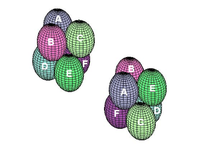
Figure 4.7: An illustration of degeneracy in DNA-coded nanoclusters.  Two different $n=6$ isomers are pictured, both with the same minimal second moment configuration, the octahedron.  

Chapter 5 Programmable Self-Assembly

5.1 Introduction

Over recent years, significant attention has been attracted to the possibility of nanotechnological applications of DNA [18], [17], [46], [47], [48].  Among the various proposals, one of the most interesting directions is the use of DNA–mediated interactions for programmable self–assembly of nanoparticle structures [25], [15], [45], [44]. Several schemes of such self-assembly have been studied both experimentally and theoretically. Their common theme is the use of colloidal particles functionalized with specially designed ssDNA (markers), whose sequence defines the particle type. In such systems, selective type-dependent interactions can be introduced either by making the markers complementary to each other, or by using linker-DNA chains whose ends are complementary to particular marker sequences.

Recent theoretical studies have addressed the expected phase behavior [56], melting properties [2], and morphological diversity [55] of DNA–colloidal assemblies.  In particular, there are indications that these techniques can be utilized for fabrication of photonic band gap materials [74], [75].  Despite significant experimental progress, the long-term potential of DNA–based self–assembly is far from being realized.  For instance, most of the experimental studies of DNA–colloidal systems report random aggregation of the particles [53].  Some degree of structural control in these systems has been achieved, mostly by varying the relative sizes of particles, rather than by tuning the interactions [43], [16].

In the present chapter [65], we take a broader view of programmable self-assembly.  While this theoretical study is strongly motivated by the prospects of DNA-colloidal systems, our main objective is to address a more general question: how well can a desired structure be encoded by tunable interactions between its constituents? The particular model system on which we focus consists of distinguishable particles with individually controlled interactions between any pair of them. In the first stage of our study, we analyze a simplified yet generic version of such a system.  All the particles have the same repulsive potential, while the attraction is introduced only between selected pairs of particles in the form of a spring-like quadratic potential.  This potential mimics the effect of a stretchable DNA molecule whose ends can selectively adsorb to the particular pair of particles.  We then introduce a number of additional features which make the model a more realistic description of an actual DNA-colloidal system.

Our major result is that a combination of stretchable interparticle linkers (e.g. sufficiently long DNA), and a soft repulsive potential greatly reduces (or totally eliminates) the probability of self-assembling an undesired structure.  The experimental prototype is a system of particles in a mixture of two types of DNA molecules which can selectively adsorb to the particle surface.  The first type are DNA molecules with two ”sticky” ends, i.e. both end sequences of the DNA are complementary to the particle marker sequence.  With one end adsorbed to the particle surface, the remaining sticky end makes it possible to introduce an attractive interparticle potential between selected particle pairs.  The second type are DNA molecules with one sticky end which adsorbs to the particle surface.  These DNA strands give rise to a soft repulsive potential of entropic origin between all particle pairs.

There is a natural analogy between our problem and the folding of proteins where interactions between amino acids encode the overall structure.  However, it should be emphasized that the task of programmable self-assembly in colloidal systems is even more demanding than protein folding: any intermediate metastable configuration has a much longer lifetime and therefore means a misfolding event.  Because of this, we were looking for a self–assembly scenario which does not require thermally activated escape from a metastable configuration. This makes the problem additionally interesting from the theoretical perspective of ”jamming”, a phenomenon actively studied in the context of granular and colloidal systems. Our results can be interpreted in terms of a jamming-unjamming transition controlled by the interaction parameters.

It should be emphasized that the goal of this work is primarily conceptual, as opposed to providing a manual for the immediate experimental realization of ordered colloidal structures.  Nevertheless, future experimental schemes will be forced to overcome obstacles presented by colloidal jamming.  With this in mind, one of the most salient features of our model is the ability to smooth the energy landscape by tuning the interactions between particles.

The plan for the chapter is as follows.  In section 2, we address the problem within a simplified generic model which mimics the nanoparticle system with stretchable DNA connections. An unexpected and very encouraging result of this study is that the misfolding (or jamming) in the model system can be completely avoided for a certain set of parameters.  In section 3 the original model is adapted to a more realistic situation which incorporates the random character of the DNA-mediated interactions.  In section 4 we discuss the prospects for the future experimental implementation of our scheme.  In section 5 we summarize the major results.

5.2 Beads and Springs Model

Consider an isolated group of repulsive particles linked via a polymer spring to their desired nearest neighbours.  We assume that the DNA marker sequence is the same for any two markers attached to the same particle, but different particles have different marker sequences (i.e. each particle has a unique code).  In this case, the attraction between any two particles can be effectively switched on by adding DNA ”linkers” whose ends are complementary to the corresponding marker sequences of the particles.  As a first approach to the problem, we introduce a generic ”Beads & Springs” model which incorporates essential features of the DNA–nanoparticle system.  The model system contains $N$ particles with pairwise (type-independent) repulsive potential $U(r)$.  In general, this repulsion may have a hard-core or soft-core behavior, or be a combination of the two. In order to model the DNA–induced type–dependent attraction, we introduce a harmonic potential (linear springs) which acts only between selected pairs of particles [22].  Thus, the model Hamiltonian has the following form:

$$H=\frac{1}{2}\sum\limits_{\alpha,\beta}\kappa J_{\alpha\beta}\left|\mathbf{r}_{\alpha}-\mathbf{r}_{\beta}\right|^{2}+U(|\mathbf{r}_{\alpha}-\mathbf{r}_{\beta}|)$$ (5.1)

Here $\alpha,\beta$ are the particle indices, $\mathbf{r}_{\alpha}$ are their current positions, and $\kappa$ is the spring constant.  The connectivity matrix element $J_{\alpha\beta}$ may be either 1 or 0, depending on whether the two particles are connected by a spring, or not.  Our goal is to program the desired spatial configuration by choosing an appropriate connectivity matrix $J_{\alpha\beta}$. A natural construction is to put $J_{\alpha\beta}=1$ for any pair of particles which must be nearest neighbors in the desired cluster, and not to connect the particles otherwise (i.e. put $J_{\alpha\beta}=0$).  This construction assures that the target configuration is the ground state of the system.

Note that our problem is somewhat similar to that of heteropolymer folding.  In that case, the selective interactions between monomers (e.g. amino acids in protein) are responsible for the coding of the spacial structure of a globule. Our major concern is whether the kinetics of the system will allow it to reach the ground state within a reasonable time.   Unfortunately, since the Brownian motion of a typical nanoparticle is relatively slow (compared to molecular time scales), it is unrealistic to expect that our system will be able to find the target configuration by ”hopping” between various metastable states, as in the case of protein folding.  However, our case is different because the attractive force grows with distance, as opposed to the short–range nature of heteropolymer self–interactions.  As we shall see below, this difference is essential, making it possible for the system to reach the ground state without stopping at any metastable configuration.

We have performed a molecular dynamics simulation of the above model by numerically integrating its Langevin equation:

$$b^{-1}\mathbf{\dot{r}}_{\alpha}=-\mathbf{\nabla}_{\alpha}H+\mathbf{\eta}_{\alpha}$$ (5.2)

Here $b$ is the particle mobility.  The thermal noise has been artificially suppressed in this study (i.e. $\eta=0$ ).  In other words, we have assumed the worst case scenario: once the system is trapped in a local energy minimum, it stays there indefinitely. The equations of motion were solved numerically by a first order Runge-Kutta method.  First, we studied a system of $N=49$ distinguishable particles in 2D, whose native configuration was a $7\times 7$ square cluster (see Figure 5.1).  Their initial positions were random, and the connectivity matrix was constructed according to the above nearest–neighbor rule.

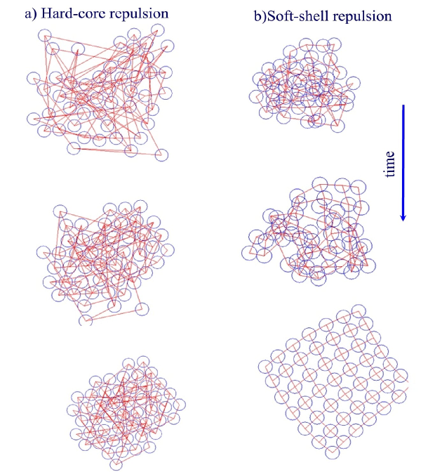
Figure 5.1: Programmable self–assembly in 2D, studied within the Beads & Springs model. 49 particles are all distinct and connected with linear springs to encode the desired configuration (7x7 square). The jamming behavior is observed for the case of hard spheres (a). However, the assembly of the target structure can be achieved if the repulsion is sufficiently ”soft” (b).

First, we studied the case when $U(r)$ is a hard–core potential. More precisely, the repulsive force was given by a semi–linear form:

$$f_{hc}\left(r\right)=-\frac{\partial U_{hc}\left(r\right)}{\partial r}=\kappa_{0}(d-r)\Theta(d-r)$$ (5.3)

Here $\Theta$ is the unit step function, and $d$ is the diameter of the hard sphere.  The parameter $\kappa_{0}$ determines the strength of the hard-core repulsion, and it does not affect the results, as long as $\kappa_{0}\gg\kappa$.  In our simulations, we found that the hard sphere system eventually stops in a configuration definitely different from the desired one, a behavior which is well known in the context of granular and colloidal systems as ”jamming” [88].  Remarkably, the jamming can be avoided when the hard-core repulsion is replaced by a soft–core potential:

$$U_{sc}(r)=U_{0}\exp(-r/\lambda).$$ (5.4)

Here the decay length $\lambda$ is of the order of the equilibrium interparticle distance $r_{0}$.  This indicates that the energy landscape can be made smooth by a combination of long-range selective attraction and soft-core repulsion.

The result is surprising and remarkably robust.  In particular, in order to expand our finding to the 3D case, we studied the self-assembly of particles into tetrahedra of various sizes ($N=10,20,35$).  This time, the hard core interaction potential was superimposed with a soft shell repulsion, which makes the model more relevant for an actual DNA-colloidal system:

$$U\left(r\right)=U_{hc}\left(r\right)+U_{sc}\left(r\right).$$ (5.5)

After the system has fully relaxed, a geometric measure of the folding success is determined by comparing particle separations of the desired final state to those generated from a set of random initial conditions. Figure 5.2 shows the ”jamming phase diagram” for these systems.  To assign a point on the diagram to the correct folding regime, we required 100 consecutive successful folds.  While this criterion can only give an upper bound on the jamming probability (which is approximately $1\%$), an additional analysis gives strong evidence that the correct folding region of the diagram corresponds to zero probability of jamming.

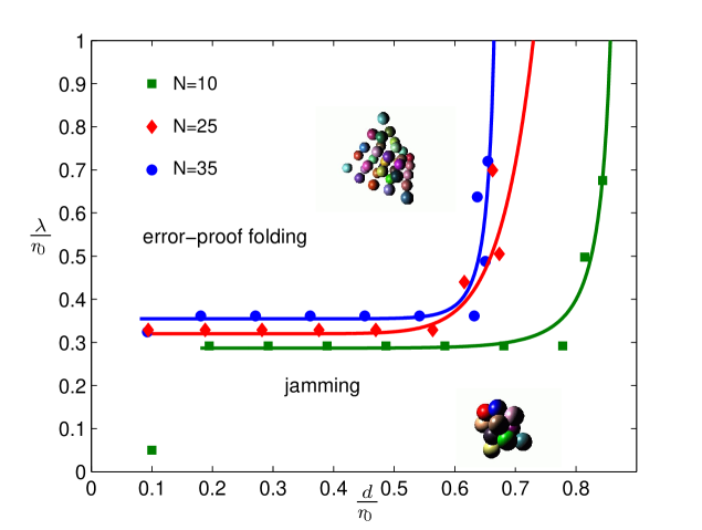
Figure 5.2: ”Jamming phase diagram” obtained for programmable self-assembly of tetrahedral clusters, within the Beads & Springs model. The control parameters depend on the equilibrium interparticle distance $r_{o}$, the diameter of the hard sphere $d$, and the range of the soft-shell repulsion $\lambda$.

5.3 Self-Assembly in DNA Colloidal Systems

As we have seen, the introduction of a soft-core repulsive potential $U_{sc}$ is crucial to a successful self-assembly proposal.  In a real system, this repulsion can be generated e.g. by DNA or another water soluble polymer adsorbed to the particle surface.  The mechanism is quite independent of the monomer chemistry, but for the sake of concreteness we will speak of the repulsion generated by DNA. Namely, we assume that a certain fraction of the DNA ”arms” of the ”octopus-like” particles are not terminated by a sticky end, and only play the role of a repulsive ”buffer”.  When the polymer coverage is sufficiently low, the interparticle repulsion is primarily due to entropy loss of a chain squeezed between two particles.  The characteristic length scale of this interaction is given by the radius of gyration of the ”buffer” chain, $R_{g}$.  The corresponding repulsive force $f_{sc}$ can be calculated exactly in the limit of relatively short buffer chains, $R_{g}\ll d$. The result of this calculation [55] can be adequately expressed in the following compact form:

$$f_{sc}\left(r\right)\approx\frac{4NR_{g}T}{d\left(r-d\right)}\exp\left(-\frac{\left(r-d\right)^{2}}{2R_{g}^{2}}\right)$$ (5.6)

Here $N$ is the total number of buffer chains per particle. Note that even though this result is only valid for $R_{g}\ll d$, it correctly captures the Gaussian decay of the repulsive force expected for longer chains as well. Therefore, we expect the results to be at least qualitatively correct beyond the regime of short buffer chains.

In addition to the modified soft potential, we have to take into account the random character of the realistic DNA-mediated attraction.  It originates from the fact that (1) the number of DNA ”arms” of the original octopus-like particles will typically be determined by a random adsorption process, and (2) the fraction of the DNA chains recruited for linking a particular pair of particles is also random.  In terms of our original model, this means that the ”springs” will not have the same spring constant.  If the individual linkers are modelled by Gaussian chains [20], the overall spring constant for a  particular pair of connected particles is given by $\kappa_{\alpha\beta}=Tm_{\alpha\beta}/2R_{g}^{{}^{\prime}2}$ , where $R_{g}^{{}^{\prime}}$ is the radius of gyration of a single linker, and $m_{\alpha\beta}$ is the number of individual chains connecting the particles.  We assume that this number obeys the generic Poisson distribution:  $P(m)=\overline{m}^{m}e^{-\overline{m}}/m!$.  As formulated, the model is cast as a system of coupled differential equations:

$$\mathbf{\dot{r}}_{\alpha}=b\sum\limits_{\beta}\left[-\frac{T}{2R_{g}^{{}^{\prime}2}}J_{\alpha\beta}m_{\alpha\beta}r_{\alpha\beta}+f_{hc}\left(r_{\alpha\beta}\right)+f_{sc}\left(r_{\alpha\beta}\right)\right]\mathbf{\hat{n}}_{\alpha\beta}$$ (5.7)

Here $r_{\alpha\beta}=\left|\mathbf{r}_{\alpha}-\mathbf{r}_{\beta}\right|$, $\mathbf{\hat{n}}_{\alpha\beta}=\left(\mathbf{r}_{\alpha}-\mathbf{r}_{\beta}\right)/r_{\alpha\beta}$.

We have studied the behavior of the system as a function of two dimensionless parameters, one of which is the ratio of the buffer radius of gyration to the particle diameter, $R_{g}/d$ . The other parameter characterizes the relative strength of the attractive and repulsive forces:

$$\alpha=\frac{\overline{m}}{N}\left(\frac{R_{g}}{R_{g}^{{}^{\prime}}}\right)$$ (5.8)

Including the above modifications of the model, the essential result of the study is that the jamming probability can be drastically suppressed, similarly to the previous case. However, the jamming in this system cannot be eliminated completely.  Instead of an actual ”phase boundary”, we have observed a sharp crossover to the regime of predominantly good folding, in which the error probability is suppressed to a modest level $\sim 10-20\%$. Interestingly, the behavior is nearly independent of the energy parameter $\alpha$, which makes $R_{g}/d$ the only major control parameter. Figure 5.3 shows the error probability as a function of this geometric parameter for tetrahedral clusters of different sizes. As this plot indicates, the misfolding behavior gets suppressed as $R_{g}/d$ exceeds $1$.

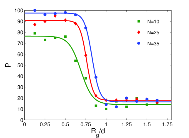
Figure 5.3: Error probability $P$ as a function of aspect ratio $R_{g}/d$ for tetrahedral clusters with modified soft-potential and realistic DNA-mediated attraction. Each data point on the misfolding profile represents 100 trials.  

As a further test of the robustness of the model, we consider a modified attractive potential which deviates from the linear Hooke’s law.  For larger forces we enter the Pincus regime [24], where the end-to-end extension of the polymer chain $r$ is related to the external tension $f\sim$ $r^{\frac{3}{2}}$.  This tension law incorporates the excluded volume interaction of individual linker DNA with themselves, which was not previously considered.  Remarkably, the major result for error suppression carries over, as illustrated in figure 5.4.

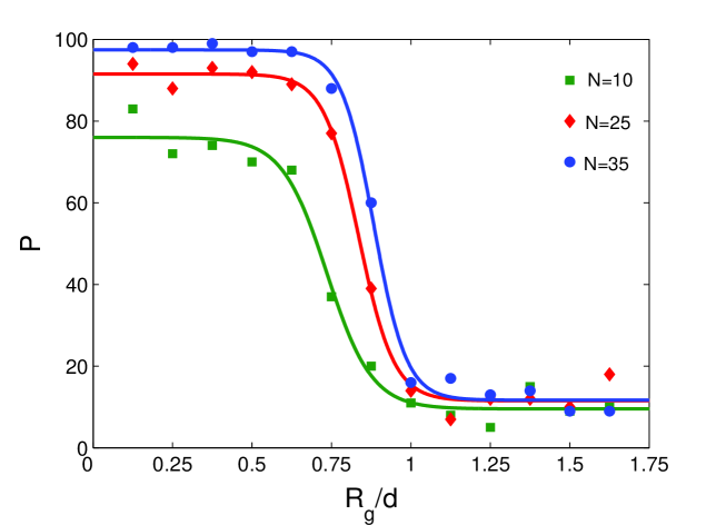
Figure 5.4: Error probability $P$ as a function of aspect ratio $R_{g}/d$ for tetrahedral clusters in the Pincus regime.  Each data point on the misfolding profile represents 100 trials.  

Our description has several limitations which are to be addressed in future work.   In particular, our discussion is only applicable to the limit of modest coverage of particles with buffer chains. This case of weakly overlapping adsorbed chains (known as the ”mushroom regime”) is drastically different from the high–coverage ”polymer brush” behavior [21].   Nevertheless, our major conclusions appear to be rather robust.  The condition for error suppression($R_{g}/d\gtrsim 1$) is the same in both the harmonic and Pincus regimes.

In the previous chapter we presented a detailed discussion of a method to self-assemble DNA-coded clusters.  Within the context of the beads and springs model presented here we can discuss the role that jamming plays in preventing the one anchor structures from assuming the minimal second moment configuration.  We performed simulations of the assembly of optimal colloidal clusters up to $n=9$ particles by numerically integrating the particles’ Langevin equations.  As indicated in Figure 5.5, the hard sphere system gets trapped in a configuration with a larger $M_{2}$ than the optimal cluster, whereas the soft-core system is able to fully relax.  The jamming behavior is largely determined by the single control parameter $\frac{R_{g}}{d}$, with $d$ the diameter of the hard sphere.  Beyond the critical value $\frac{R_{g}}{d}\gtrsim.5$ the jamming behavior is either completely eliminated, or greatly reduced in the case of larger clusters.

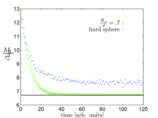
Figure 5.5: Plot of the dimensionless second moment $\frac{M_{2}}{r_{o}^{2}}$ as function of time for $n=9$ particles.  Results are shown for the case of hard spheres and also for a system with a soft-core repulsion with geometric parameter $\frac{R_{g}}{d}=.7$.  The dashed line is the theoretical moment for the triaugmented triangular prism, which is the minimal $n=9$ structure.  

5.4 Discussion

Previous studies have demonstrated an experimental implementation of self–assembly in a DNA–colloidal system [1], [26].  The approach in these studies differs from our vision of controllable self-assembly in two major ways: (1) because the ”linker” DNA chains($\sim 20nm$) used are much shorter than the particle diameter($\sim 1\mu m$), the particles behave as sticky spheres, and (2) there is little diversity in particle type, where the structures result from interactions of a one or two component system.  We would like to discuss issues related to a future experimental implementation similar to the modified Beads & Springs model.

In our molecular dynamics simulations we assumed that (1) the desired group of particles has already been localized in a small region of space, and that (2) the interparticle connections have already been made.  There are a number of experimental challenges associated with implementing the self-assembly proposal of our simulations.  In another manuscript [61] we provide a detailed discussion of the localization problem, which is the first major experimental intermediary.

After localization, the next step is to make the desired connections between particles within the cluster.  To do so one can add short ssDNA with sequences $\bar{s}_{A}\bar{s}_{B}$ to link particles $A$ and $B$.  The DNA marker sequence $s_{A}$ for particle $A$ is a sequence of nucleotides complementary to the $\bar{s}_{A}$ portion of the linker sequence $\bar{s}_{A}\bar{s}_{B}$.  The hydrogen bonding of complementary nucleotides forms base pairs which join both marker strands to the linker, creating a DNA bridge between the two particles.  After the interparticle links are formed, they should be made permanent by ligation.  Since the spring constants of the above dsDNA chains are too small to drive the self-assembly of a desired cluster, we propose to melt them either by changing the temperature or pH. As a result, the dsDNA links will be turned into ssDNA with a much higher effective spring constant (due to the shorter persistence length).  This will trigger the self–assembly scenario similar to the one discussed within the Beads & Springs model.  Note that DNA entanglements may be effectively eliminated if the procedure is done in the presence of DNA Topoisomerases.

5.5 Summary

We presented a model of DNA-colloidal self-assembly which exhibits a tunable jamming-unjamming transition.  The combination of a soft-core repulsion with a type-dependent long range attraction provides a natural funneling of the energy landscape to the ground state configuration.  This is to be contrasted with the case of protein folding, where under physiological conditions the interactions between amino acids are screened to several angstroms.  Because this lengthscale is much shorter than the spatial extent of the native structure, large regions of the energy landscape are flat, which prohibits formation of the native state on the basis of funneling alone.  As a result the folding rate is necessarily limited by the diffusion of amino acid segments looking for their desired nearest neighbors [89], [90].  The fact that the potential in the DNA-colloidal system is long ranged is essential, allowing us to avoid the pitfall of slow particle diffusion.

Within the Beads and Springs Model, we obtained the jamming phase diagram for several modest sized tetrahedral clusters.  We identified a regime of parameter space with error-proof folding, and demonstrated the importance of introducing a soft-core repulsion.  The original model was then adapted to include several features of realistic DNA-mediated interactions.  Although the jamming cannot be completely eliminated in the modified system, we identified a regime of predominantly good folding, and calculated the error probability for tetrahedral clusters.  The jamming behavior is determined by a single geometric parameter $R_{g}/d$.  We concluded by discussing prospects for an experimental implementation of our self-assembly scheme.

Chapter 6 Cooperativity Based Drug Delivery Systems

6.1 Introduction

Nanoparticle based drug delivery systems have attracted substantial attention for their potential applications in cancer treatment [7], [8], [9], [10], [91].  It is hoped that by selectively targeting cancer cells with chemotherapeutic agents one can reduce side effects and improve treatment outcomes relative to other drug delivery systems which do not discriminate between normal and cancerous cells.  For example, many epithelial cancer cells are known to overexpress the folate receptor [92], [6], [93], [94], [95].  A nanoparticle with many folic acid ligands will preferentially bind to cancerous cells.  A recent study [4] of a potential drug delivery platform consisting of generation 5 PAMAM dendrimers with different numbers of folic acid found that multivalent interactions have a pronounced effect on the dissociation constant $K_{D}$.  This enhancement is the signature for cooperativity of the binding, which should lead to a greater specificity to cancerous cells in vivo.

In this chapter [96] we present a theoretical study of these key-locking nanodevices (see Fig. 6.1).  We introduce the idea that there are kinetic limitations to cooperativity-based drug delivery systems.  In vivo the finite timescale for endocytosis prevents arbitrarily high cooperativity in the drug delivery system.  To begin we provide a detailed analysis of the in vitro experiments [4].  Although enhancement of the association is the signature of greater cooperativity, in this case it is due mostly to non-specific binding of the dendrimers to the surface.  Due to the finite time window of the experiments, only indirect support can be offered to the notion of enhanced cooperativity.  In the latter half of the chapter we expand the notion of kinetically limited cooperativity to the system in vivo.  The equilibrium coverage of nanodevices on the cells is related to the concentration of folate-binding proteins and the strength of the key-lock binding.  We quantify the preferential adsorption of nanodevices to the cancerous cells, and discuss how kinetic effects prohibit arbitrarily high cooperativity in the drug delivery system.  The implications of the work for designing new drug delivery vehicles with enhanced specificity to cancerous cells are discussed.

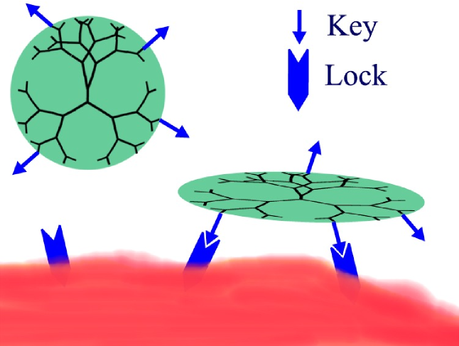
Figure 6.1: A picture of the dendrimer ”key-lock” binding to the cell membrane surface.  

6.2 Key-Lock Model

We now consider a simple model of the nanodevice system.  A dendrimer with a maximum of $M$ keys (e.g. folic acids) interacts with locks (e.g. folate-binding proteins) in the cell membrane surface.  A simple order of magnitude estimate for $M\simeq 30$ can be obtained from the ratio of the surface area of the dendrimer to the surface area of the folic acid.  In this way we implicitly take into account the excluded volume effect between the keys.  The free energy for the dendrimer connected to the surface by $m$ key-lock bridges is [30]

$$F_{m}=-Tm\Delta\text{.}$$ (6.1)

The dimensionless energy parameter $\Delta$ contains information about the binding energy of a single key-lock pair, and the entropy loss associated with localizing a dendrimer on the cell-membrane surface.  An estimate of $\Delta\simeq 17.5$ can be obtained from the dissociation constant of free folic acid $K_{D}^{(o)}$ using the equilibrium relation between the dissociation constant and the free energy change for the formation of a single key-lock bridge, $K_{D}^{(o)}=\frac{1}{\xi^{3}}\exp(-\Delta)$.  Here $\xi^{3}$ is the localization volume of an ”unbound” key.  Below we determine the value $\xi\simeq 0.2nm$ from analysis of the in vitro experiments, which was used to determine $\Delta$.

The measured association rate constant $k_{a}$ of the dendrimer with folic acid is a factor of $10^{3}$ times greater than $k_{a}^{(o)}$ of free folic acid.  Only a factor of $\overline{m}$ can be attributed to the dendrimer having many folic acids attached to it.  Here $\overline{m}$ is the average number of keys attached to the dendrimer.  This pronounced enhancement of $k_{a}$ is the primary evidence for non-specific attraction between the dendrimer and the surface.

$$k_{a}=\overline{m}k_{a}^{(o)}\exp\left(\frac{-\epsilon_{0}}{T}\right)$$ (6.2)

The non specific attraction $\epsilon_{0}$ accounts for the Van der Waals attraction to the surface and hydrophobic enhancement.  The experimentally measured $k_{a}$ values are reproduced by a reasonable energy scale $-\epsilon_{0}\simeq 7T$ (see Fig. 6.2).

We provide a simple explanation for the experimentally observed dependence of the dissociation rate constant $k_{d}$ on $\overline{m}$.  The dissociation rate constant of free folic acid $k_{d}^{(o)}\sim 10^{-5}\left[s^{-1}\right]$ provides a characteristic departure time of $1/k_{d}^{(o)}\simeq 30$ $hours$ for those dendrimers attached by a single key-lock bridge.  Moreover, the departure time for multiple bridge states increases exponentially in $\Delta$, for two bridges it is $\exp(\Delta)/k_{d}^{(o)}\simeq 10^{9}$ $hours$.  Strictly speaking the relaxation is multiexponential, with time constants for each bridge number.  However, the experimental $k_{d}$ values are well fit by a single exponential.  On the timescale of the experiment, we will only see the departure of dendrimers attached by a single bridge.

The experiment measures the departure rate of dendrimers which are connected to the surface by a single bridge, but are unable to form an additional connection.  Consider a dendrimer attached to the surface by one key-lock bridge.  If the dendrimer has a total of $j$ keys, the probability that none of the remaining $j-1$ keys can form bridges is $(1-\alpha)^{j-1}$.  We now compute the probability $\alpha$ that a remaining key is available to form a bridge.  In the vicinity of the surface the dendrimer is a disclike structure [97] with radius $a\simeq 4.8nm$.  By rotation of the dendrimer about the first bridge, a key located at position $\rho$ searches the annulus of area $2\pi\rho\xi$ to find a lock.  The probability of encountering a lock in this region is $2\pi\rho\xi\sigma_{o}$, where the surface density of the locks $\sigma_{o}\simeq\frac{16}{100nm^{2}}$.  By averaging over the key location we obtain the final result

$$\alpha=\frac{1}{a}\int_{0}^{a}2\pi\rho\xi\sigma_{o}d\rho\simeq\xi a\sigma_{o}.$$ (6.3)

Assuming that during dendrimer preparation the attachment of folic acid to the dendrimer is a Poisson process, the probability of a dendrimer having exactly $j$ keys is $P_{j}(\overline{m})=\exp(-\overline{m})\overline{m}^{j}/j!$.  The final result is obtained by averaging the probability that no additional bridges can form over this distribution.  The factor of $j$ counts the number of ways to make the first connection.

$$k_{d}=k_{d}^{(o)}\frac{\sum\limits_{j=1}^{\infty}(1-\alpha)^{j-1}jP_{j}(\overline{m})}{\sum\limits_{j=1}^{\infty}jP_{j}(\overline{m})}=k_{d}^{(o)}\exp(-\alpha\overline{m})$$ (6.4)

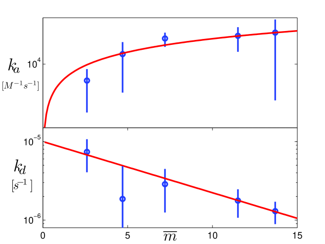
Figure 6.2: Top: Plot of the association rate constant (Eq. 6.2) $k_{a}[M^{-1}s^{-1}]$ versus $\overline{m}$.  Bottom: Plot of the effective dissociation rate constant (Eq. 6.4) $k_{d}[s^{-1}]$ versus $\overline{m}$.  In the fit $k_{d}^{(o)}=10^{-5}[s^{-1}]$ and $\alpha=0.15$.  The experimental data points are taken from Figure 5 in [4].

The formula predicts an exponential decay of the effective dissociation rate constant with the average number of folic acids on the dendrimer, which allows for a quantitative comparison to the experiment (see Fig. 6.2).  Using $\alpha\simeq 0.15$, we can determine the localization length $\xi\simeq 0.2nm$ for locks in the experiment from Eq. 6.3.  This estimate for $\xi$ is physically reasonable, and comparable to the bond length of the terminal group on the dendrimer.

Similar to the finite timescale of the experiments in vitro [4], in vivo the endocytosis time provides kinetic limitations to cooperative binding.  In equilibrium the concentration of dendrimers on the cell surface $n$ is related to the concentration of dendrimers in solution $c_{sol}$ through the association constant $K_{A}=n/(\sigma_{o}c_{sol})$.  Although it is tempting to use our in vitro results to define the association constant as $K_{A}=k_{a}/k_{d}$, this approach is only valid provided there is a single rate for both association and dissociation.  Because the dendrimer can form multiple bridges, there are many different rate constants.  We present a partition function method which accounts for the multiple rate constants in the problem, and for the possibility that in vivo there is surface diffusion of locks.

6.3
Calculation of the Association Constant $K_{A}$

In this section we consider the reaction $\sigma_{o}+c_{sol}\rightleftharpoons n$ for which the association constant $K_{A}$ is defined as

$$K_{A}=\frac{n}{\sigma_{o}c_{sol}}.$$ (6.5)

Here $\sigma_{o}$ is the concentration of locks in the cell membrane, $c_{sol}$ is the concentration of dendrimers in solution, and $n$ is the concentration of dendrimers attached to the surface of the cell membrane.  To proceed we construct a vector $\mathbf{s}$ of length $M$, which is a list of the possible sites folic acid can attach to the dendrimer.  If a folic acid is present at site $i$ we have $s_{i}=1$, and otherwise $s_{i}=0$.  The concentration of dendrimers on the cell surface $n$ is proportional to the partition function of the system.

$$n=\frac{c_{sol}\xi^{3}}{A}\sum\limits_{m=1}^{m_{\max}}\int\frac{d^{2}\mathbf{r}_{1}\cdots d^{2}\mathbf{r}_{m}}{m!}\sum_{i\neq j\neq\cdots\neq p}s_{i}\cdots s_{p}$$ (6.6)

$$\times\sigma(\mathbf{r}_{1})\cdots\sigma(\mathbf{r}_{m})\exp\left[m\Delta-\frac{\epsilon_{0}+\varepsilon_{ij\cdots p}(\mathbf{r}_{1},\cdots,\mathbf{r}_{m})}{T}\right]$$

Here $\sigma(\mathbf{r})$ is the surface density of locks on the cell membrane at position $\mathbf{r}$, and $A$ denotes the total area of the cell membrane.  The energy $\varepsilon_{ij\cdots p}(\mathbf{r}_{1},\cdots,\mathbf{r}_{m})$ that appears in the Boltzmann weight is the elastic energy penalty required to form multiple bridges.  The point is that in solution the dendrimer is roughly spherical, but must flatten to a pancake like shape to form multiple connections with the cell surface [97].

The ensemble averaging is performed by assuming that during nanodevice preparation the attachment of folic acid to the dendrimer is a Poisson process.   In this case $\left\langle s_{i}\right\rangle=\frac{\overline{m}}{M}$ is given by the success probability that a folic acid attaches to the dendrimer, and the$\ m$ point correlator $\left\langle s_{i}s_{j}\cdots s_{p}\right\rangle=\left(\frac{\overline{m}}{M}\right)^{m}$.  In other words, the probability of attachment of a given folic acid to a terminal group on the dendrimer is unaffected by the presence of other folic acids up to an exclusion rule which has already been taken into account.  If the interaction potential between locks in the cell membrane is $V(\mathbf{r}_{1,}\cdots,\mathbf{r}_{m})$ we have $\left\langle\sigma(\mathbf{r}_{1})\cdots\sigma(\mathbf{r}_{m})\right\rangle=\left(\sigma_{o}\right)^{m}\exp\left[-V(\mathbf{r}_{1,}\cdots,\mathbf{r}_{m})/T\right]$.  By performing the ensemble averaging we arrive at the result for the equilibrium coverage $n_{m}^{eq}$ of dendrimers connected to the cell surface by $m$ bridges.  Since the lock which forms the first bridge can be anywhere on the cell membrane, without loss of generality we place this lock at $\mathbf{r}_{1}=\mathbf{0}$.  The integrand is then independent of $\mathbf{r}_{1}$, and the first areal integration gives a factor of the cell surface area $A$.

$$\left\langle n\right\rangle = \frac{c_{sol}\xi^{3}}{A}A\sum_{m=1}^{m_{\max}}\int\frac{d^{2}\mathbf{r}_{2}\cdots d^{2}\mathbf{r}_{m}}{m!}\left\langle\sigma\mathbf{(0)}\sigma\mathbf{\mathbf{(r}}_{2}\mathbf{\mathbf{)}\cdots}\sigma\mathbf{(r}_{m}\mathbf{)}\right\rangle\times$$

$$\sum_{i\neq j\neq\cdots\neq p}\left\langle s_{i}\cdots s_{p}\right\rangle\exp\left(m\Delta-\frac{\epsilon_{0}+\varepsilon_{ij\cdots p}(\mathbf{0},\cdots,\mathbf{r}_{m})}{T}\right)$$

$$\left\langle n\right\rangle = c_{sol}\xi^{3}\sum_{m=1}^{m_{\max}}\int\frac{d^{2}\mathbf{r}_{2}\cdots d^{2}\mathbf{r}_{m}}{m!}\left(\sigma_{o}\right)^{m}\exp\left[\frac{-V(\mathbf{0},\mathbf{\mathbf{r}}_{2},\cdots,\mathbf{r}_{m})}{T}\right]\times$$

$$\sum_{i\neq j\neq\cdots\neq p}\left(\frac{\overline{m}}{M}\right)^{m}\exp\left(m\Delta-\frac{\epsilon_{0}+\varepsilon_{ij\cdots p}(\mathbf{0},\mathbf{r}_{2},\cdots,\mathbf{r}_{m})}{T}\right)$$

$$\left\langle n\right\rangle = c_{sol}\xi^{3}\exp\left(\frac{-\epsilon_{0}}{T}\right)\sum_{m=1}^{m_{\max}}\frac{\left(\overline{m}\sigma_{o}\exp(\Delta)\right)^{m}}{m!}\frac{\xi^{2(m-1)}}{\xi^{2(m-1)}}\frac{1}{M^{m}}\times$$

$$\sum_{i\neq j\neq\cdots\neq p}\int d^{2}\mathbf{r}_{2}\cdots d^{2}\mathbf{r}_{m}\exp\left[-\frac{(V(\mathbf{0},\mathbf{\mathbf{r}}_{2},\cdots,\mathbf{r}_{m})+\varepsilon_{ij\cdots p}(\mathbf{0},\mathbf{r}_{2},\cdots,\mathbf{r}_{m}))}{T}\right]$$

Here $K_{A}^{(o)}=1/K_{D}^{(o)}$ $=\xi^{3}\exp(\Delta)$ is the association constant of free folic acid which has been measured experimentally.

$$\left\langle n\right\rangle = \frac{c_{sol}\xi^{3}}{\xi^{2}}\sum_{m=1}^{m_{\max}}\frac{\left(\overline{m}\sigma_{o}\xi^{2}\exp(\Delta)\right)^{m}}{m!}\exp\left[\frac{-\left(\epsilon_{0}+\epsilon_{el}^{(m)}\right)}{T}\right]=$$

$$c_{sol}\xi\sum_{m=1}^{m_{\max}}\frac{1}{m!}\left(\frac{\overline{m}\sigma_{o}K_{A}^{(o)}}{\xi}\right)^{m}\exp\left[\frac{-\left(\epsilon_{0}+\epsilon_{el}^{(m)}\right)}{T}\right]$$

This gives the final result for the ensemble averaged concentration of dendrimers on the surface $\left\langle n\right\rangle$:

$$\left\langle n\right\rangle = \sum_{m=1}^{m_{\max}}n_{m}^{eq}$$ (6.11)

$$n_{m}^{eq} = \frac{c_{sol}\xi}{m!}\left(\frac{\overline{m}\sigma_{o}K_{A}^{(o)}}{\xi}\right)^{m}\exp\left[\frac{-\left(\epsilon_{0}+\epsilon_{el}^{(m)}\right)}{k_{B}T}\right]$$ (6.12)

Here the elastic energy $\epsilon_{el}^{(m)}$ is defined by:

$$\exp\left(\frac{-\epsilon_{el}^{(m)}}{T}\right) \equiv \frac{1}{M^{m}}\int\frac{d^{2}\mathbf{r}_{2}\cdots d^{2}\mathbf{r}_{m}}{\xi^{2(m-1)}}$$

$$\times\sum_{i\neq j\neq\cdots\neq p}\exp\left[-\frac{(V(\mathbf{0},\mathbf{\mathbf{r}}_{2},\cdots,\mathbf{r}_{m})+\varepsilon_{ij\cdots p}(\mathbf{0},\mathbf{r}_{2},\cdots,\mathbf{r}_{m}))}{T}\right]$$

Defined in this manner, $\exp(-\epsilon_{el}^{(m)}/T)$ has a physical interpretation as the Boltzmann weight for the elastic energy of the optimal $m$ bridge configuration.  The membrane surface can only accommodate a finite number of locks in the vicinity where the dendrimer is attached [4].  As a result $n_{m}^{eq}=0$ for $m>m_{\max}$ since forming additional key-lock pairs would require deforming the dendrimer into configurations prohibited by elastic stress and steric hindrance.

The calculation of the equilibrium coverage above is applicable with and without diffusion of locks in the cell membrane.  In the regime of fast diffusion the locks are free to diffusively explore the surface.  Their positions are ergodic variables, and the overall ensemble averaged equilibrium coverage counts the Boltzmann weights for different lock configurations.  In the regime of slow diffusion, locks are immobilized in the cell membrane.  This is the relevant situation when the locks have phase separated into protein rich (lipid rafts) and protein poor phases.

6.4 Kinetically Limited Cooperativity

When kinetic effects are taken into account, these two regimes are drastically different.  When locks are diffusing, the dendrimer is able to attain the maximum cooperativity $m_{\max}$.  After the dendrimer makes the first connection, it simply waits for locks to diffuse in the vicinity of available keys to make additional connections.  In the absence of diffusion, the optimal configuration can only be obtained by multiple binding and unbinding events, the timescale for which is prohibitively long.  This is the case for lipid rafts where the locks are immobilized similar to the experiments in vitro [4], and the dendrimer is unable to attain the maximum cooperativity.  This is the kinetic origin of limited cooperativity in the drug delivery system.

We now quantify the preferential attachment of nanodevices to the cancerous cells, taking into account kinetic effects.  Let $n_{m}$ denote the concentration of dendrimers attached to the cell by $m$ bridges.  We can construct a differential equation for $n_{m}$ by considering linear response to the deviation from thermal equilibrium $n_{m}^{eq}$.

$$\frac{dn_{m}}{dt}=k_{d}^{(m)}(n_{m}^{eq}-n_{m})-\gamma n_{m}$$ (6.14)

Here $\gamma$ is the rate for endocytosis [98].  The dissociation rate constant $k_{d}^{(m)}$ for breaking all $m$ bridges is:

$$k_{d}^{(m)}=m\frac{k_{a}^{(o)}}{\xi^{3}}\exp\left(\frac{\epsilon_{el}^{(m)}}{T}\right)\exp(-m\Delta)$$ (6.15)

The steady state concentration $n_{m}^{ss}$ is the solution to $\frac{dn_{m}}{dt}=0$.  As a result we obtain the total coverage $n$ of dendrimers on the cell surface in the following form:

$$n=\sum_{m=1}^{m_{\max}}n_{m}^{ss}=\sum_{m=1}^{m_{\max}}\frac{n_{m}^{eq}}{1+\gamma/k_{d}^{(m)}}$$ (6.16)

We now have a means to discuss the preferential attachment of dendrimers to the cancerous cell.  The folate binding proteins on the cancerous cell are overexpressed, i.e. if their concentration on the normal cell is $\sigma_{o}$, their concentration on the cancerous cell is $r\sigma_{o}$ with $r>1$.  The value of $r$ is determined by the biology, and cannot be changed by the experimenter.  To quantify the preferential binding of the dendrimer to the cancerous cells we calculate the ratio of coverage on cancerous to normal cells $\frac{n(r\sigma_{o})}{n(\sigma_{o})}$.  Values of this ratio greater than $r$ indicate the nature of cooperative dendrimer binding (see Fig. 6.3).

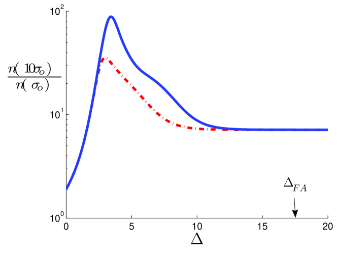
Figure 6.3: The ratio of surface concentrations of dendrimers on cancerous to normal cells $\frac{n(10\sigma_{o})}{n(\sigma_{o})}$ as a function of $\Delta$ with $r=10$.  The dotted line corresponds to an endocytosis time $1/\gamma=1\left[hr\right]$ and the solid line is $1/\gamma=10\left[hr\right]$.  Here $\overline{m}=15$, $m_{\max}=4$, $\xi=3[nm]$, and $\sigma_{o}=2\times 10^{-3}[nm^{-2}]$.  $\varepsilon_{el}^{(m)}=3T$ for $m\geq 3$ bridges.  

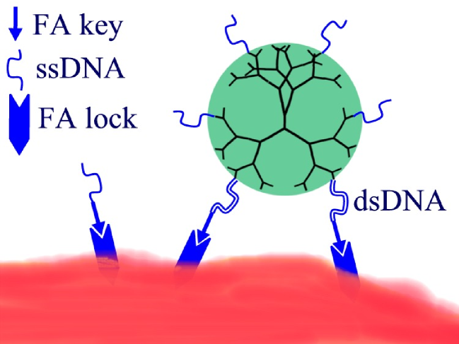
Figure 6.4: Single-stranded DNA (ssDNA) on the dendrimer hybridize to the ssDNA attached to the folic acid (FA) key.  

6.5 Design of an Improved Drug-Delivery Platform

The current experimental scheme uses direct targeting with folic acid ($\Delta_{FA}\simeq 17.5$), which does not optimize the coverage on cancerous cells.  By decreasing $\Delta$ the drug delivery can be tuned to the favorable regime.  To do so, consider binding to the cell through an intermediary, perhaps single-stranded DNA (ssDNA).  Instead of folic acid, attach many identical sequences of ssDNA to the dendrimer.  Then, one also constructs a folic acid-ssDNA complex with the ssDNA sequence complementary to that of the ssDNA attached to the dendrimer.  The folic acid will bind very strongly to the folic acid receptors on the cell membrane, leaving the unhybridized ssDNA as a receptor (see Fig. 6.4).  Effectively one has replaced $\Delta_{FA}$ with a new value $\Delta_{DNA}$ which can be tuned very precisely by controlling the length and sequence of the DNA.  Due to the large degree of overexpression [92], this change substantially increases the ratio of dendrimers on cancerous to normal cells.  As indicated in Fig. 6.3, with $r\simeq 10$ there is a $5$ fold improvement over direct targeting with folic acid!

6.6 Summary

In this chapter we presented a theoretical study of a cell-specific, targeted drug delivery system.  A simple ”key-lock” model was proposed to determine the effective dissociation rate and association rate constants of the dendrimers as a function of the average number of folic acids, which permits a direct comparison to the experimental results.  The equilibrium coverage of dendrimers on the cell surface was calculated, and the differences between in vitro experiments and in vivo studies were discussed.  The degree of cooperativity of the drug delivery system is kinetically limited.  We quantified the notion of preferential selection of dendrimers to cancerous cells, and demonstrated that the selectivity can be enhanced by decreasing the strength of individual bonds.  A particular implementation of this idea using ssDNA was discussed.

Chapter 7 Conclusions and Perspectives

7.1 The Relationship Between Crystallization and Jamming

After the publication of [65] two recent studies reported the self-assembly of colloidal crystals using DNA mediated interactions [29], [28], [54].  Up until this point most of the studies reported aggregation of colloids into disordered, amorphous aggregates [1] or close packed crystals [26].  In these earlier studies polystyrene spheres of diameter $d\sim 1\mu m$ were grafted with dsDNA of length $L\simeq 20nm$.  Because $L<l_{p}\simeq 50nm$ for dsDNA the DNA linkers behaved effectively as rigid rods.  The essential change in the new studies was to work with flexible ($L\gg l_{p}$) DNA with contour length $L\gtrsim d$.  For this purpose Gang et al. [29] grafted $g\simeq 60$ ssDNA onto gold nanoparticles of diameter $d\simeq 11nm$.  Interestingly, they found that as one varies the length $L\simeq Na$ of the DNA ($a\simeq.43nm$ for ssDNA [99]), the system goes from a disordered to crystalline configuration.  Increasing the lengthscale for the repulsive interactions between particles provides a means to smooth the energy landscape to the equilibrium body-centered cubic configuration.

It seems that an important control parameter in such systems is the ratio $\xi/d$ where $\xi$ is the lengthscale for the repulsion and $d$ is the hard sphere diameter.  In fact it has been theoretically predicted that one can obtain different crystalline morphologies by varying this control parameter [55].  This control parameter is something we have already encountered in chapter 5.  There $\xi\simeq R_{g}$ was the radius of gyration of the buffer DNA.  Of course a direct analogy between the two systems is not possible, as the self-assembly of a modest number of particles into colloidal clusters is quite different than the crystallization problem.  Motivated by their similarities, it is at least plausible that the explanation for which systems are able to attain their ground state configuration and which remain ”jammed” in metastable configurations is qualitatively similar.

To proceed with such a comparison we have to determine an appropriate definition of the control parameter.  Here I propose that by defining $\xi\simeq R$ one might be able to obtain a qualitative understanding of which systems crystallize and which remain disordered in terms of a critical value of the control parameter $R/d$.  Here $R$ is the so-called ”coronal thickness” for a polymer brush attached to a small colloidal particle $d\ll R$.  To determine $R$ we consider a simple scaling argument of Daoud and Cotton [100], [39].  By balancing the osmotic pressure against the polymer elasticity we obtain

$$\frac{1}{2}c^{2}a^{3}T\simeq\frac{kRg}{4\pi R^{2}}\text{.}$$ (7.1)

Assuming that the monomer concentration takes its average value $c=(Ng)/V$ with $V=(4\pi R^{3})/3$ yields the result for the coronal thickness

$$R\simeq g^{\frac{1}{5}}N^{\frac{3}{5}}a\text{.}$$ (7.2)

We are now in a position to compare the value of the control parameter for the different systems studied experimentally [29].

Table 7.1: Control Parameters for Equilibrium Colloidal Crystallization

$N$	$R/d$	Aggregate?
$18$	$0.48$	amorphous
$30$	$0.66$	amorphous
$40$	$0.78$	amorphous
$50$	$0.89$	crystalline
$65$	$0.95$	crystalline

It is interest to note this approximation gives a critical value of the control parameter $\frac{R}{d}\gtrsim 0.9$, which is very close to the critical value given for the self-assembly of colloidal clusters in chapter 5.  The value $N=40$ is the mean for a system prepared with particles of type $A$ for which $N_{A}=50$ and particles of type $B$ for which $N_{B}=30$.  All other systems were prepared in a homogeneous fashion with $N_{A}=N_{B}=N$.  This analogy seems to indicate that the system with shorter ssDNA is trapped in a metastable configuration analogous to the jammed configuration for the colloidal clusters, and the introduction of a long-range repulsive potential provides a kinetically feasible pathway to the equilibrium configuration.  One topic for future research would be a more detailed consideration of the jamming analogy in colloidal crystals beyond the crude scaling argument given here.  Comparison of the results to the experiments of [29] is potentially problematic, since they increase the length of the DNA but keep the grafting density constant for all systems studied.  As a result the properties of the polymer brush that forms on the particle surface likely vary for different linker lengths.

7.2 Building Up Complexity

Studies on DNA-mediated colloidal crystallization have emphasized the importance of thermal annealing as a means to facilitate crystallization.  Here we explore another idea which might assist in the equilibrium DNA-mediated self-assembly of colloidal crystals.  The approach, which to date has received little attention in experimental studies, is to self-assemble crystalline structures in a hierarchical fashion (see Fig. 7.1).  Consider a binary system of particles with two colors $A$ and $B$.  The DNA marker sequences are chosen so that $AB$ bonds form as a result of DNA hybridization, but not $AA$ or $BB$.  To take advantage of this cohesive energy, the nearest neighbours in the resulting crystalline morphologies should be of different color [55].  These types of crystal structures are commonly described as a lattice with a basis [101].  For example, one can consider placing $A$ and $B$ type particles at the points of a body-centered cubic lattice so that each particle has $8$ nearest neighbours of the opposite type.  This structure, sometimes called the cesium chloride structure, is obtained by taking a simple cubic lattice with a basis consisting of an $A$ type particle at the origin and a $B$ type particle at the center of the cube $\left(a/2\right)(\mathbf{x}+\mathbf{y}+\mathbf{z})$.  Here $a$ is the lattice constant and the primitive lattice vectors are $\mathbf{x=(}\begin{array}[]{ccc}1&0&0\end{array})$, $\mathbf{y=(}\begin{array}[]{ccc}0&1&0\end{array})$, and $\mathbf{z=(}\begin{array}[]{ccc}0&0&1\end{array})$.  Similarly one may obtain the sodium chloride structure where the particles are located at the vertices of a simple cubic lattice and each particle has $6$ nearest neighbours of the opposite type.  This crystal structure can be described as a face centered cubic lattice with a basis.

In fact, the same is true of more exotic crystal structures, for example the diamond structure.  This structure, the same as that adopted by gallium arsenide, can be described as a face-centered cubic lattice with a two particle basis.  The diamond structure is of particular interest for its potential applications in the self-assembly of photonic band gap materials [74].  Since these crystal structures can be built up by as $AB$ pairs, one could attempt to assemble these crystals where the fundamental units are not individual particles but dimers.  The dimers could be assembled first and then used as the fundamental components.

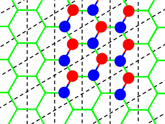
Figure 7.1: Building up a honeycomb structure using dimers.  The honeycomb can be viewed as a two dimensional triangular lattice with a two particle basis.  

Alternatively one could consider grafting two different types of DNA onto the $A$ and $B$ type particles.  DNA with sequence $A_{1}$ is chosen complementary to DNA with sequence $B_{1}$ and $A_{2}$ is chosen complementary to $B_{2}$.  By varying the length of the recognition sequence, one can tune the melting temperatures $T_{1}$ and $T_{2}$ for the $A_{1}B_{1}$ and $A_{2}B_{2}$ complexes.  In fact, the experimenter can control the relative grafting density of the strands on the particles [37].  By choosing a low grafting density for the $A_{2}$ and $B_{2}$ strands, the system will behave in an interesting fashion.  For temperatures $T>T_{2}$ the particles will be dispersed as monomers.  As the temperature is lowered $T_{1}<T<T_{2}$ we expect to see the formation of predominantly dimers.  Finally, for $T<T_{1}$ we expect aggregation of large clusters, and under appropriate conditions crystallization.  The hope is that this intermediate stage in the assembly might facilitate faster crystallization, i.e. provide a kinetically feasible pathway to the equilibrium ground state.

This is just one example of how complexity can be incorporated into the DNA-colloidal system.  Other examples have already been considered earlier in the thesis, for example the self-assembly of DNA coded clusters.  There we saw the potential advantages of working with a multiple colored system, as opposed to most of the experimental studies to date which have worked with at most two colors.  These ideas naturally lead us to the next topic, the inverse problem in self-assembly.

7.3 The Inverse Problem in Self-Assembly

A natural extension of these ideas is to consider the so-called inverse problem in self-assembly.  Presume that you have a particular target structure $S$ in mind.  For example, this structure might be a particular crystalline morphology, or clusters with prescribed geometrical features.  Given $S$, the goal is to determine the set of components $C$ who self-assemble into $S$.  The DNA grafted colloids considered in this thesis, or combinations thereof, constitute a particularly promising component class due to the diversity and complexity of the potential interactions.  This procedure requires knowledge of the interaction potential which governs the dynamics between components.  Some progress has been made on the inverse problem for isotropic colloidal systems which interact through a pair potential [102], [103], [104], [105].  This work determined a class of designer potentials which give rise to a number of crystal structures, in both two and three dimensions.  The drawback to this approach is that the designer potentials are generally quite complex.  They contain a large number of numerical fitting constants, so it is not known how the designer potentials could be realized experimentally.

A first step towards understanding the inverse problem in the DNA-colloidal system is to determine the pair potential for two colloids grafted with DNA.  Some steps in this direction include [26], [37], [106].  In general one would have to consider the effects of anisotropy.  The major goal is to understand how the experimental variables (grafting density of DNA, DNA flexibility and length, hybridization free energy, etc.) affect the interaction potential.  By tuning these variables one might be able to construct potentials which mimic the designer potentials determined through Monte Carlo simulations.  Of course knowledge of the potential which gives rise to a particular equilibrium structure is only part of the problem.  The free energy landscape is generally quite rugged, so one has to take care to provide a feasible pathway to reach the ground state configuration on experimental timescales.  Future studies which combine insights drawn from experiment, theory, and modeling will hopefully lead to a realization of the incredible technological potential of DNA-colloidal systems.

Appendix A Bridging Probability for Scheme B

In this appendix we calculate $c_{eff}$ for scenario B (see Fig. 2.1).  Taking the $z$ direction normal to the planar surfaces separated by a distance $2h$, an eigenfunction expansion [67] yields the following expression for the probability distribution function.  Here $\beta\equiv\frac{\pi^{2}R_{g}^{2}}{24h^{2}}$, and $N$ is the normalization (unimportant for our purposes).

$$P(\mathbf{r},\mathbf{r}^{\prime})=NP_{X}(x,x^{\prime})P_{Y}(y,y^{\prime})P_{Z}(z,z^{\prime})$$ (A.1)

$$P_{X}(x,x^{\prime}) = \exp\left(-\frac{3}{2R_{g}^{2}}(x-x^{\prime})^{2}\right)$$ (A.2)

$$P_{Y}(y,y^{\prime}) = \exp\left(-\frac{3}{2R_{g}^{2}}(y-y^{\prime})^{2}\right)$$ (A.3)

$$P_{Z}(z,z^{\prime}) = \sum_{n=1}^{\infty}\sin\left(\frac{n\pi z}{2h}\right)\sin\left(\frac{n\pi z^{\prime}}{2h}\right)\exp\left[-\beta n^{2}\right]$$ (A.4)

To circumvent the Dirichlet boundary conditions, we start the chains at a small distance $\lambda$ from the planes.  We then have $\mathbf{r}_{1}^{\prime}=(x_{1}^{{}^{\prime}},y_{1}^{{}^{\prime}},\lambda)$ and $\mathbf{r}_{2}^{\prime}=(x_{2}^{{}^{\prime}},y_{2}^{{}^{\prime}},2h-\lambda)$.  We first expand the distribution functions to first order in $\lambda$ and then perform the integration over all the possible hybridized conformations $\mathbf{r}_{1}=\mathbf{r}_{2}$.

$$P_{1} \equiv P(\mathbf{r}_{1},\mathbf{r}_{1}^{\prime}=(x_{1}^{{}^{\prime}},y_{1}^{{}^{\prime}},\lambda))=\frac{N\pi\lambda}{2h}P_{X}(x_{1},x_{1}^{{}^{\prime}})P_{Y}(y_{1},y_{1}^{{}^{\prime}})\times$$

$$\sum_{n=1}^{\infty}n\sin\left(\frac{n\pi z_{1}}{2h}\right)\exp\left[-\beta n^{2}\right]$$

$$P_{2} \equiv P(\mathbf{r}_{2},\mathbf{r}_{2}^{\prime}=(x_{2}^{{}^{\prime}},y_{2}^{{}^{\prime}},2h-\lambda))=-\frac{N\pi\lambda}{2h}P_{X}(x_{2},x_{2}^{{}^{\prime}})P_{Y}(y_{2},y_{2}^{{}^{\prime}})\times$$

$$\sum_{m=1}^{\infty}(-1)^{m}m\sin\left(\frac{m\pi z_{2}}{2h}\right)\exp\left[-\beta m^{2}\right]$$

The integration over the $x_{1}$ and $y_{1}$ components are Gaussian, which leaves the integration in the direction normal to the plane.

$$\int P_{1}P_{2}\delta^{3}(\mathbf{r}_{1}-\mathbf{r}_{2})d^{3}\mathbf{r}_{1}d^{3}\mathbf{r}_{2} =-\frac{N^{2}\pi^{3}\lambda^{2}R_{g}^{2}}{12h^{2}}\sum_{n=1}^{\infty}\sum_{m=1}^{\infty}(-1)^{m}nmI_{nm}(h)\exp\left[-\beta(n^{2}+m^{2})\right]$$ (A.7)

$$I_{nm}(h) \equiv\int_{0}^{2h}\sin\left(\frac{n\pi z_{1}}{2h}\right)\sin\left(\frac{m\pi z_{1}}{2h}\right)dz_{1}=h\delta_{n,m}$$ (A.8)

The second line follows since $m$ and $n$ are integers, using $\lim_{\delta\rightarrow 0}\frac{\sin\delta}{\delta}=1$.  Defining $\mathbf{\Delta r}^{{}^{\prime}}\equiv\mathbf{r}_{1}^{\prime}-\mathbf{r}_{2}^{\prime}$ the numerator in the expression for $c_{eff}$ is:

$$\int P(\mathbf{r}_{1},\mathbf{r}_{1}^{\prime})P(\mathbf{r}_{2},\mathbf{r}_{2}^{\prime})\delta^{3}(\mathbf{r}_{1}-\mathbf{r}_{2})d^{3}\mathbf{r}_{1}d^{3}\mathbf{r}_{2}$$

$$= -\frac{N^{2}\pi^{3}\lambda^{2}R_{g}^{2}}{12h}\exp\left[-\frac{3}{4}\left(\frac{\mathbf{\Delta r}^{{}^{\prime}}}{R_{g}}\right)^{2}\right]\sum\limits_{n=1}^{\infty}(-1)^{n}n^{2}\exp[-2\beta n^{2}]$$

We also make use of the following result.

$$\int P_{1}d^{3}\mathbf{r}_{1}=\frac{4N\pi\lambda R_{g}^{2}}{3}\sum_{k=1\text{, }k\text{\ }odd}^{\infty}\exp\left[-\beta k^{2}\right]$$ (A.10)

This leads us to the overlap density for complementary, flexible linkers with $x=\frac{h}{R_{g}}$.

$$c_{eff} = \frac{c(x)}{R_{g}^{3}}\exp\left[-\frac{3}{4}\left(\frac{\mathbf{\Delta r}^{{}^{\prime}}}{R_{g}}\right)^{2}\right]$$ (A.11)

$$c(x) = \frac{-3\pi}{64x}\frac{\sum\limits_{n=1}^{\infty}(-1)^{n}n^{2}\exp\left[-2\beta n^{2}\right]}{\left(\sum\limits_{k=1\text{, }k\text{\ }odd}^{\infty}\exp\left[-\beta k^{2}\right]\right)^{2}}$$ (A.12)

When the chains are strongly compressed, $\beta\sim\frac{1}{x^{2}}\gg 1$, the asymptotic behavior of $c(x)$ is easily determined as the sums converge rapidly.  The more interesting physical regime is as particles approach at separations large compared to the radius of gyration of the marker strands, which is $\beta\ll 1$.  To extract the asymptotics in this regime we can massage the summation as follows.

$$\sum\limits_{n=1}^{\infty}(-1)^{n}n^{2}\exp[-2\beta n^{2}] = \frac{-1}{2}\frac{\partial}{\partial\beta}\sum\limits_{n=1}^{\infty}(-1)^{n}\exp[-2\beta n^{2}]=$$

$$\frac{-1}{2}\frac{\partial}{\partial\beta}\left[2\sum\limits_{n=1}^{\infty}\exp[-8\beta n^{2}]-\sum\limits_{n=1}^{\infty}\exp[-2\beta n^{2}]\right]$$

$$\sum\limits_{k=1\text{, }k\text{\ }odd}^{\infty}\exp\left[-\beta k^{2}\right] = \sum\limits_{k=1}^{\infty}\exp\left[-\beta k^{2}\right]-\sum\limits_{k=1}^{\infty}\exp\left[-4\beta k^{2}\right]$$ (A.14)

Then note that for any even function of n, $f(n)$ we have:

$$\sum_{n=1}^{\infty}f(n)=\frac{1}{2}\left(\sum_{n=-\infty}^{\infty}f(n)-f(0)\right)$$ (A.15)

Finally we use an identity derived from properties of the theta function [107].

$$\sum_{n=-\infty}^{\infty}\exp\left[-\beta n^{2}\right]=\sqrt{\frac{\pi}{\beta}}\sum_{n=-\infty}^{\infty}\exp\left[\frac{-\pi^{2}n^{2}}{\beta}\right]$$ (A.16)

Expanding the sums using these identities, the result of some straightforward but tedious algebra gives the asymptotic behavior of the binding probability.

$$\Delta\widetilde{G}_{B} \simeq \Delta G_{B}+T\left[\begin{array}[]{c}\frac{3}{4}\left(\frac{\Delta r^{{}^{\prime}}}{R_{g}}\right)^{2}+\log\left(R_{g}^{3}c_{o}\right)+\log\left(\frac{32}{\pi^{2}}\right)\\ +3\log(x)+\frac{\pi^{2}}{12x^{2}}\end{array}\right]\text{ \ for }x\ll 1$$ (A.19)

$$\Delta\widetilde{G}_{B} \simeq \Delta G_{B}+T\left[\begin{array}[]{c}\frac{3}{4}\left(\frac{\Delta r^{{}^{\prime}}}{R_{g}}\right)^{2}+\log\left(R_{g}^{3}c_{o}\right)-\log\left(\frac{9}{4}\sqrt{\frac{3}{\pi}}\right)\\ -2\log(x)+3x^{2}\end{array}\right]\text{ \ for }x\gg 1$$ (A.22)

Appendix B Bridging Probability for Scheme C

In this appendix we calculate $c_{eff}$ for scenario C (see Fig. 2.1).  If the method of images is used to construct the probability distribution function for the flexible linker DNA, as opposed to the eigenfunction expansion used in Appendix A, we arrive at the following expression [67].

$$P(\mathbf{r},\mathbf{r}^{\prime}) = NP_{X}(x,x^{\prime})P_{Y}(y,y^{\prime})P_{Z}(z,z^{\prime})$$ (B.1)

$$P_{Z}(z,z^{\prime}) = \sum_{n=-\infty}^{\infty}\left\{\exp\left[\frac{-3}{2R_{g}^{2}}(z-z^{\prime}-4nh)^{2}\right]-\exp\left[\frac{-3}{2R_{g}^{2}}(z+z^{\prime}-4nh)^{2}\right]\right\}$$ (B.2)

$$\simeq \exp\left[\frac{-3}{2R_{g}^{2}}(z-z^{\prime})^{2}\right]-\exp\left[\frac{-3}{2R_{g}^{2}}(z+z^{\prime})^{2}\right]$$

Since $\zeta\equiv\frac{L}{R_{g}}\gg 1$ we only need the $n=0$ term in the expression for $P_{Z}(z,z^{\prime})$.  $P_{X}(x,x^{\prime})$ and $P_{Y}(y,y^{\prime})$ are the same as in Appendix A(equation A.1).  Once again we start the chains at a small distance $\lambda$ from the planes.  The majority of the hybridized conformations will have the planar surfaces separated by approximately the linker length $L$.  To simplify the discussion we take $\mathbf{\Delta r}^{{}^{\prime}}=0$ from the beginning of the calculation, which corresponds to orientations of the rigid linker with a small component parallel to the surface.  We then have $\mathbf{r}_{1}^{\prime}=(0,0,\lambda)$ and $\mathbf{r}_{2}^{\prime}=(0,0,L+\Delta-\lambda)$.  We first expand the distribution functions to first order in $\lambda$ and then perform the integration over all the possible hybridized conformations $|\mathbf{r}_{1}-\mathbf{r}_{2}|=L$.

$$P_{1} \equiv P(\mathbf{r}_{1},\mathbf{r}_{1}^{\prime}=(0,0,\lambda))=\frac{6\lambda N}{R_{g}^{2}}P_{X}(x_{1},0)P_{Y}(y_{1},0)z_{1}\exp\left[\frac{-3z_{1}^{2}}{2R_{g}^{2}}\right]$$ (B.3)

$$P_{2} \equiv P(\mathbf{r}_{2},\mathbf{r}_{2}^{\prime}=(0,0,L+\Delta-\lambda)=\frac{6\lambda N}{R_{g}^{2}}P_{X}(x_{2},0)P_{Y}(y_{2},0)\times$$

$$(L+\Delta-z_{2})\exp\left[\frac{-3(L+\Delta-z_{2})^{2}}{2R_{g}^{2}}\right]$$

To impose the delta function constraint we write:

$$z_{2} = z_{1}+L\cos\theta$$ (B.5)

$$y_{2} = y_{1}+L\sin\theta\sin\phi$$ (B.6)

$$x_{2} = x_{1}+L\sin\theta\cos\phi$$ (B.7)

$$\int\delta(|\mathbf{r}_{1}-\mathbf{r}_{2}|-L)d^{3}\mathbf{r}_{2} \Rightarrow L^{2}\int\sin\theta d\theta d\phi$$ (B.8)

The integrations over $x_{1}$ and $y_{1}$ are Gaussian.  There is no azimuthal dependence, so the $\phi$ integration gives a factor of $2\pi$.  We also need the following integral:

$$\int P_{1}d^{3}\mathbf{r}_{1}=\frac{4N\pi\lambda R_{g}^{2}}{3}$$ (B.9)

We define $\epsilon\equiv\frac{\Delta}{L}$ and $z\equiv\frac{z_{1}}{L}$.  Since we consider DNA bridges with the rigid linker aligned with a small component parallel to the planar surfaces, the upper bound for the polar integration is given by $\theta_{\max}\simeq\frac{1}{\zeta}$.

$$c_{eff}(\mathbf{\Delta r}^{{}^{\prime}} = 0)\simeq\frac{27\zeta^{3}}{8\pi R_{g}^{3}}\int\limits_{0}^{\frac{1}{\zeta}}\sin\theta\exp\left[-\frac{3}{4}\zeta^{2}\sin^{2}\theta\right]I_{z}(\theta,\epsilon,\zeta)d\theta$$ (B.10)

$$I_{z}(\theta,\epsilon,\zeta) = \int\limits_{0}^{1+\epsilon}dz(1-\cos\theta+\epsilon-z)z$$

$$\times\exp\left[-\frac{3}{2}\zeta^{2}\left\{z^{2}+(1-\cos\theta+\epsilon-z)^{2}\right\}\right]$$

We first calculate the $z$ integration $I_{z}(\theta,\epsilon,\zeta)$.  Since we consider all of the possible conformations of the short linkers between planes, we can see that the upper bound for the $z$ integration is $z_{\max}=1+\epsilon$.  However, since $\zeta\gg 1$ the gaussian decay allows us to extend the integration to $\infty$.  We define $f\equiv z-\frac{\beta}{2}$ and the small parameter $\beta\equiv 1-\cos\theta+\epsilon$.  Completing the square gives:

$$I_{z}(\theta,\epsilon,\zeta)\simeq\exp\left[-\frac{3}{4}\zeta^{2}\beta^{2}\right]\int\limits_{-\frac{\beta}{2}}^{\infty}\left(\frac{\beta^{2}}{4}-f^{2}\right)\exp\left[-3\zeta^{2}f^{2}\right]df$$ (B.12)

Since $\beta$ is small we take the lower bound for the integration to $0$.

$$I_{z}(\theta,\epsilon,\zeta)\simeq\exp\left[-\frac{3}{4}\zeta^{2}\beta^{2}\right]\frac{1}{4\zeta}\sqrt{\frac{\pi}{3}}\left(\frac{\beta^{2}}{2}-\frac{1}{3\zeta^{2}}\right)$$ (B.13)

We now expand the $\theta$ integrand in terms of the small parameters $\theta\sim\epsilon\sim\frac{1}{\zeta}$.

$$c_{eff}(\mathbf{\Delta r}^{{}^{\prime}} = 0)\simeq\frac{27}{32\sqrt{3\pi}R_{g}^{3}}\exp\left[-\frac{3}{4}\zeta^{2}\beta^{2}\right]\left(\frac{\zeta^{2}\epsilon^{2}}{2}-\frac{1}{3}\right)$$

$$\times\int\limits_{0}^{\frac{1}{\zeta}}\theta\exp\left[-\frac{3}{4}\zeta^{2}(1+\epsilon)\theta^{2}\right]d\theta$$

$$= \frac{9\left(1-e^{-\frac{3}{4}}\right)}{32\sqrt{3\pi}R_{g}^{3}}\exp\left[-\frac{3}{4}\zeta^{2}\epsilon^{2}\right]\left(\epsilon^{2}-\frac{2}{3\zeta^{2}}\right)$$ (B.15)

$$\Delta\widetilde{G}_{C}(\mathbf{\Delta r}^{{}^{\prime}}=0)\simeq\Delta G_{C}+T\left[\begin{array}[]{c}\log\left(R_{g}^{3}c_{o}\right)+\log\left(\frac{32\sqrt{3\pi}}{9\left(1-e^{-\frac{3}{4}}\right)}\right)+\frac{3}{4}\zeta^{2}\epsilon^{2}\\ -\log\left(\epsilon^{2}-\frac{2}{3\zeta^{2}}\right)\end{array}\right]$$ (B.16)

We are interested in the minimum free energy with respect to the separation between planar surfaces, determined by $\frac{\partial\Delta\widetilde{G}_{C}(\mathbf{\Delta r}^{{}^{\prime}}=0)}{\partial\epsilon}=0$.  Performing the differentiation we find $\epsilon^{\ast}=\frac{\sqrt{2}}{\varsigma}$.

$$\Delta\widetilde{G}_{C}(\mathbf{\Delta r}^{{}^{\prime}} = 0,\epsilon=\epsilon^{\ast})\simeq\Delta G_{C}+T\log\left[\frac{8\sqrt{\frac{\pi}{3}}L^{2}R_{g}c_{o}}{\left(e^{-\frac{3}{2}}-e^{-\frac{9}{4}}\right)}\right]$$ (B.17)

$$= \Delta G_{C}+4.24T+T\log\left[L^{2}R_{g}c_{o}\right]$$ (B.18)

BIBLIOGRAPHY

BIBLIOGRAPHY

- [1] Valignat, M.-P.; Theodoly, O.; Crocker, J. C.; Russel, W. B.; Chaikin, P. M. PNAS 2005, 102, 4225-4229.
- [2] Jin, R.; Wu, G.; Li, Z.; Mirkin, C. A.; Schatz, G. C. JACS 2003, 125, 1643-1654.
- [3] Manoharan, V. N.; Elsesser, M. T.; Pine, D. J. Science 2003, 301, 483-487.
- [4] Hong, S.; Leroueil, P. R.; Majoros, I. J.; Orr, B. G.; Jr., J. R. B.; Holl, M. M. B. Chemistry and Biology 2007, 14, 107-115.
- [5] Moore, G. E. Electronics 1965, 38,.
- [6] Ross, J. F.; Chaudhuri, P. K.; Ratnam, M. Cancer 1994, 73, 2432-2443.
- [7] Hilgenbrink, A. R.; Low, P. S. J. Pharm. Sci. 2005, 94, 2135-2146.
- [8] Lu, Y. J.; Low, P. S. Adv. Drug Deliv. Rev. 2002, 54, 675-693.
- [9] Stella, B.; Arpicco, S.; Peracchia, M. T.; Desmaele, D.; Hoebeke, J.; Renoir, M.; D’Angelo, J.; Cattel, L.; Couvreur, P. J. Pharm. Sci. 2000, 89, 1452-1464.
- [10] Quintana, A.; Raczka, E.; Piehler, L.; Lett, I.; Myc, A.; Majoros, I.; Patri, A. K.; Thomas, T.; Mule, J.; Jr., J. R. B. Pharm. Res. 2002, 19, 1310-1316.
- [11] Park, S.-J.; Taton, T. A.; Mirkin, C. A. Science 2002, 295, 1503.
- [12] Vora, G. J.; Meador, C. E.; Stenger, D. A.; Andreadis, J. D. Appl Environ Microbiol. 2004, 70, 3047-3054.
- [13] Call, D. R. Critical Reviews in Microbiology 2005, 31, 91-99.
- [14] Ito, T.; Okazaki, S. Nature 2000, 406, 1027-1031.
- [15] Seeman, N. C. Nature 2003, 421, 427-431.
- [16] Soto, C. M.; Srinivasan, A.; Ratna, B. R. JACS 2002, 124, 8508-8509.
- [17] Ball, P. Nature 2001, 413, 667-668.
- [18] Seeman, N. C. Angew. Chem. Int. Ed. 1998, 37, 3220-3238.
- [19] Seeman, N. C. Int. J. Nanotechnology 2005, 2, 348-370.
- [20] Grosberg, A. Y.; Khokhlov, A. Statistical Physics of Macromolecules; AIP, New York: AIP Press, American Institute of Physics, 500 Sunnyside Boulevard, Woodbury, NY 11797-2999, 1994.
- [21] de Gennes, P. Scaling Concepts of Polymer Physics; Cornell University Press, Ithaca, NY: Ithaca, NY, 1979.
- [22] Jones, R. A. L. Soft Condensed Matter; Oxford University Press: Great Clarendon Street, Oxford OX2 6DP, U.K., 2003.
- [23] Flory, P. Principles of Polymer Chemistry; Cornell University Press: Ithaca, N.Y., 1971.
- [24] Pincus, P. Macromolecules 1976, 9, 386-388.
- [25] Mirkin, C. A.; Letsinger, R. L.; Mucic, R. C.; Storhoff, J. J. Nature 1996, 382, 607 - 609.
- [26] Biancaniello, P. L.; Kim, A. J.; Crocker, J. C. PRL 2005, 94, 058302.
- [27] Park, S. Y.; Stroud, D. Phys. Rev. B. 2003, 67, 212202.
- [28] Park, S. Y.; Lytton-Jean, A. K. R.; Lee, B.; Weigand, S.; Schatz, G. C.; Mirkin, C. A. Nature 2008, 451, 553-556.
- [29] Nykypanchuk, D.; Maye, M. M.; van der Lelie, D.; Gang, O. Nature 2008, 451, 549-552.
- [30] Licata, N. A.; Tkachenko, A. V. Phys. Rev. E 2006, 74, 041408.
- [31] Israelachvili, J. N. Intermolecular and Surface Forces; Academic Press: London, 1985.
- [32] Safran, S. A. Statistical Thermodynamics of Surfaces, Interfaces, and Membranes; Westview Press: Boulder, CO, 2003.
- [33] Derjaguin, B. V.; Landau, L. Acta Physicochimica 1941, 14, 633.
- [34] Verwey, E. J.; Overbeek, J. T. G. Theory of the Stability of Lyophobic Colloids; Elsevier: Amsterdam, 1947.
- [35] Bell, G. M.; Levine, S.; McCartney, L. N. J. Colloid Int. Sci. 1970, 33, 335.
- [36] Manning, G. S. J. Chem. Phys. 1969, 51, 924.
- [37] Nykypanchuk, D.; Maye, M. M.; van der Lelie, D.; Gang, O. Langmuir 2007, 23, 6305-6314.
- [38] de Gennes, P. G. Macromolecules 1980, 13, 1069-1075.
- [39] Pincus, P. Macromolecules 1991, 24, 2912-2919.
- [40] Milner, S. T.; Witten, T. A. Macromolecules 1988, 21, 2610-2619.
- [41] Milner, S. T. Science 1991, 251, 905-914.
- [42] Alivisatos, A. P.; Peng, X.; Wilson, T. E.; Johnsson, K. P.; Loweth, C. J.; Jr., M. P. B.; Schultz, P. G. Nature 1996, 382, 609.
- [43] Milam, V. T.; Hiddessen, A. L.; Crocker, J. C.; Graves, D. J.; Hammer, D. A. Langmuir 2003, 19, 10317-10323.
- [44] Cobbe, S.; Connolly, S.; Ryan, D.; Nagle, L.; Eritja, R.; Fitzmaurice, D. J. Phys. Chem. B 2003, 107, 470-477.
- [45] Winfree, E.; Liu, F.; Wenzler, L. A.; Seeman, N. C. Nature 1998, 394, 539-544.
- [46] Braun, E.; Eichen, Y.; Sivan, U.; Ben-Yoseph, G. Nature 1998, 391, 775-778.
- [47] Wengel, J. Org. Biomol. Chem 2004, 2, 277-280.
- [48] Dwyer, C.; Johri, V.; Cheung, M.; Patwardhan, J.; Lebeck, A.; Sor, D. Nanotechnology 2004, 15, 1240-1245.
- [49] Mucic, R. C.; Storhoff, J. J.; Mirkin, C. A.; Letsinger, R. L. J. Am. Chem. Soc. 1998, 120, 12674.
- [50] Mucic, R. C.; Mirkin, C. A.; Letsinger, R. L. J. Am. Chem. Soc. 2000, 122, 6305.
- [51] Braun, E.; EIchen, Y.; Sivan, U.; Ben-Yoseph, G. Nature 1998, 391, 775.
- [52] Sun, Y.; Harris, N. C.; Kiang, C.-H. Physica A 2005, 354, 1-9.
- [53] Sun, Y.; Harris, N. C.; Kiang, C.-H. Physica A 2005, 354, 1-9.
- [54] Crocker, J. C. Nature 2008, 451, 528-529.
- [55] Tkachenko, A. V. Physical Review Letters 2002, 89, 148303.
- [56] Lukatsky, D.; Frenkel, D. Physical Review Letters 2004, 92, 068302.
- [57] Zilman, A.; Kieffer, J.; Molino, F.; Porte, G.; Safran, S. A. Physical Review Letters 2003, 91, 015901.
- [58] Chen, T.; Zhang, Z.; Glotzer, S. C. PNAS 2007, 104, 717-722.
- [59] Chen, T.; Zhang, Z.; Glotzer, S. C. Langmuir 2007, 23, 6598-6605.
- [60] Chen, T.; Glotzer, S. C. Physical Review E 2007, 75, 051504.
- [61] Licata, N. A.; Tkachenko, A. V. Phys. Rev. E 2006, 74, 040401.
- [62] Chen, T.; Lamm, M. H.; Glotzer, S. C. Chemical Physics 2004, 121, 3919-3929.
- [63] Lukatsky, D. B.; Mulder, B. M.; Frenkel, D. Journal of Physics: Condensed Matter 2006, 18, S567-S580.
- [64] Storhoff, J. J.; Mirkin, C. A. Chem. Rev. 1999, 1849-1862.
- [65] Licata, N. A.; Tkachenko, A. V. Physical Review E 2006, 74, 041406.
- [66] Vainrub, A.; Pettitt, B. M. Physical Review E 2002, 66, 041905.
- [67] Dolan, A. K.; Edwards, S. F. Proceedings of the Royal Society of London. Series A, Mathematical and Physical Sciences 1974, 337, 509-516.
- [68] Thirumalai, D.; Mountain, R. D.; Kirkpatrick, T. R. Physical Review A 1989, 39, 3563-3574.
- [69] Palmer, R. G. Advances in Physics 1982, 31, 669-735.
- [70] Israelachvili, J. N. Intermolecular and Surface Forces: With Applications to Colloidal and Biological Systems; Academic Press Inc.: London, 1985.
- [71] Markham, N. R.; Zuker, M. Nucleic Acids Res. 2005, 33, W577-W581.
- [72] Licata, N. A.; Tkachenko, A. V. Phys. Rev. E 2007, 76, 041405.
- [73] Licata, N. A.; Tkachenko, A. V. Europhysics Letters 2008, 81, 48009.
- [74] Fan, S.; Villeneuve, P. R.; Joannopoulos, J. D. Phys. Rev. B 1996, 54, 11245-11251.
- [75] Sievenpiper, D. F.; Sickmiller, M. E.; Yablonovitch, E. Phys. Rev. Lett. 1996, 76, 2480-2483.
- [76] Yang, Z.-Y.; Smith, B. D. Bioconjugate Chem. 2000, 11, 805-814.
- [77] Hong, S.; Beilinska, A. U.; Mecke, A.; Keszler, B.; Beals, J. L.; Shi, X.; Balogh, L.; Orr, B. G.; Jr., J. R. B.; Holl, M. M. B. Bioconjugate Chem. 2004, 15, 774-782.
- [78] Sykes, M. F.; Glenn, M. J. Phys. A. Math. Gen. 1976, 9, 87-95.
- [79] Kehr, K.; Murthy, K.; Ambaye, H. Physics A 1998, 253, 9-22.
- [80] Stauffer, D. Introduction to Percolation Theory; Taylor and Francis: London‘, 1985.
- [81] Bouchaud, J.-P. Aging in glassy systems: new experiments, simple models, and open questions. In Soft and Fragile Matter: Nonequilibrium Dynamics, Metastability and Flow; Cates, M. E.; Evans, M. R., Eds.; IOP Publishing (Bristol and Philadelphia): Boca Raton, FL, 2000.
- [82] Scher, H.; Montroll, E. W. Physical Review B 1975, 12, 2455.
- [83] Glotzer, S. C.; Solomon, M. J. Nature Materials 2007, 6, 557-562.
- [84] Zhang, Z.; Glotzer, S. C. Nanoletters 2004, 4, 1407-1413.
- [85] Michele, C. D.; Gabrielli, S.; Tartaglia, P.; Sciortino, F. J. Phys. Chem. B 2006, 110, 8064-8079.
- [86] Smoluchowski, M. Phys. Z 1916, 17, 557-571.
- [87] Hinton, R.; Dobrota, M. Laboratory Techniques in Biochemistry and Molecular Biology. In , Vol. 6 Part 1; Elsevier/North Holland: New York, 1976; Chapter Density Gradient Centrifugation.
- [88] Segre, P.; Prasad, V.; Schofield, A.; Weitz, D. Physical Review Letters 2001, 86, 6042-6045.
- [89] Onuchic, J. N.; Luthey-Schulten, Z.; Wolynes, P. G. Annu. Rev. Phys. Chem. 1997, 48, 545-600.
- [90] McLeish, T. C. B. Biophys. J. 2005, 88, 172-183.
- [91] Choi, Y.; Mecke, A.; Orr, B. G.; Jr., J. R. B. Nanoletters 2004, 4, 391-397.
- [92] Toffoli, G.; Cernigoi, C.; Russo, A.; Gallo, A.; Bagnoli, M.; Boiocchi, M. Int. J. Cancer (Pred. Oncol.) 1997, 74, 193-198.
- [93] Weitman, S. D.; Weinberg, A. G.; Coney, L. R.; Zurawski, V. R.; Jennings, D. S.; Kamen, B. A. Cancer Res. 1992, 52, 6708-6711.
- [94] Weitman, S. D.; Lark, R. H.; Coney, L. R.; Fort, D. W.; Frasca, V.; Zurawski, V. R.; Kamen, B. A. Cancer Res. 1992, 51, 3396-3401.
- [95] Campbell, I. G.; Jones, T. A.; Foulkes, W. D.; Trowsdale, J. Cancer Res. 1991, 51, 5329-5338.
- [96] Licata, N. A.; Tkachenko, A. V. Physical Review Letters 2008, 100, 158102.
- [97] Mecke, A.; Lee, I.; Jr., J. R. B.; Holl, M. M. B.; Orr, B. G. Eur. Phys. J. E 2004, 14, 7-16.
- [98] Wiwattanapatapee, R.; Carreño-Gómez, B.; Malik, N.; Duncan, R. Pharmaceutical Research 2000, 17, 991-998.
- [99] Tinland, B.; Pluen, A.; Sturm, J.; Weill, G. Macromolecules 1997, 30, 5763-5765.
- [100] Daoud, M.; Cotton, J. J. Phys. Paris 1982, 43, 531-538.
- [101] Ashcroft, N. W.; Mermin, N. D. Solid State Physics; Harcourt College Publishers: Orlando, FL, 1976.
- [102] Rechtsman, M. C.; Stillinger, F. H.; Torquato, S. Physical Review Letters 2005, 95, 228301.
- [103] Rechtsman, M.; Stillinger, F.; Torquato, S. Physical Review E 2006, 73, 011406.
- [104] Rechtsman, M. C.; Stillinger, F. H.; Torquato, S. Physical Review E 2006, 74, 021404.
- [105] Rechtsman, M. C.; Stillinger, F. H.; Torquato, S. Physical Review E 2007, 75, 031403.
- [106] Kegler, K.; Konieczny, M.; Dominguez-Espinosa, G.; Gutsche, C.; Salomo, M.; Kremer, F.; Likos, C. N. Physical Review Letters 2008, 100, 118302.
- [107] Bellman, R. A Brief Introduction to Theta Functions; Holt, Rinehart and Winston, Inc.: New York, 1961.