Multiresolution analysis of active region magnetic structure and its correlation with the Mount Wilson classification and flaring activity

Abstract

Two different multiresolution analyses are used to decompose the structure of active region magnetic flux into concentrations of different size scales. Lines separating these opposite polarity regions of flux at each size scale are found. These lines are used as a mask on a map of the magnetic field gradient to sample the local gradient between opposite polarity regions of given scale sizes. It is shown that the maximum, average and standard deviation of the magnetic flux gradient for $\alpha,\beta,\beta\gamma$ and $\beta\gamma\delta$ active regions increase in the order listed, and that the order is maintained over all length-scales. Since magnetic flux gradient is strongly linked to active region activity, such as flares, this study demonstrates that, on average, the Mt. Wilson classification encodes the notion of activity over all length-scales in the active region, and not just those length-scales at which the strongest flux gradients are found. Further, it is also shown that the average gradients in the field, and the average length-scale at which they occur, also increase in the same order. Finally, there are significant differences in the gradient distribution, between flaring and non-flaring active regions, which are maintained over all length-scale. It is also shown that the average gradient content of active regions that have large flares (GOES class ’M’ and above) is larger than that for active regions containing flares of all flare sizes; this difference is also maintained at all length-scale. All the reported results are independent of the multiresolution transform used. The implications for the Mt. Wilson classification of active regions in relation to the multiresolution gradient content and flaring activity are discussed.

1 Introduction

Many attempts have been made to assess the complexity of active regions, as a measure of their activity. The earliest attempt (dating from 1908) - Mount Wilson classification - and still in use today, puts active regions into four broad classes, and is based on the distribution of magnetic flux polarity in the active region. The magnetic flux distribution, in relation to the location of white light sunspots, in conjunction with some simple classification rules, are used by the observer, to classify the observed region. The four main classes of active region, and their classification rules are shown in Table 1.

The success of the Mt. Wilson classification scheme lies in the fact that it is simple, and has some predictive power when combined with flare frequency rates deduced from long time series (many solar cycles) observations. Other classification schemes exist, notably the McIntosh classification scheme [McIntosh (1990)]. This is a significantly more complex classification scheme because it looks at the magnetic structure of the active region in much greater detail. This too has some predictive ability in divining activity, again based on correlation between flare frequency rates and the the McIntosh class.

Both schemes are implemented manually, and so are subject to the usual human observer biasses. Research is currently ongoing into automating these classification schemes, with some success (2006SoPh..239..519D; 2002ApJ…568..396T; 1998A.AS..131..371B). The notable feature about both the Mt. Wilson and McIntosh classification schemes is that they both use the magnetic structure, that is, the relative locations and sizes of concentrations of opposite polarity magnetic flux in the active region in order to determine active region class. Since opposite polarity flux creates gradients, these classification schemes are in essence classifying the location and size of the magnetic flux gradients in the magnetic data. Hence these classification schemes act as proxies for the magnetic flux gradient information content of the active region.

The notion of complexity is ill-defined, and that carries over to the study of active regions. Many studies have attempted to quantify the notion of active region complexity. 2005ApJ…631..628M look at around 10,000 active regions and calculate a fractal dimension for the spatial distribution of the absolute magnetic flux. Separated by Mt. Wilson class, active regions are surprisingly homogenous in fractal dimension, with very little difference between $\alpha$ class active regions and $\beta\gamma\delta$ active regions. This shows, under the assumption that the flux is a mono-fractal, that all the magnetic flux is basically the same, regardless of polarity and of what class of active region it appeared in.

The mono-fractal restriction can be removed by assuming that the magnetic flux can be described my a multifractal. This assumes that the flux can be represented by a distribution of fractals, a considerable increase in sophistication. This is physically motivated, since the multifractals have deep ties to turbulence ( 2005SoPh..228….5G; 2005SoPh..228…29A; 2002ApJ…577..487A ). conlon present the results of analyzing the multifractal content of several active regions. It is shown that the multifractal spectrum changes with the emergence of the flux, indicating that the scale content is changing with emergence. This study allows for flux cancellation in calculating the multifractal spectrum, and so implicitly takes account of the different flux polarity, a significant difference from the study of 2005ApJ…631..628M.

Both these studies are more concerned with the nature of the flux, as opposed to its gross distribution on the Sun’s surface, which is what the classification schemes outlined above deal with. In particular, these studies do not make any statements about the gradient between flux elements, which is known to be a significant indicator of activity. This study is complementary, in that it attempts to look at the spatial distribution of flux at different sizes, or length-scales, as opposed to the nature of that flux. To do this, the study uses four multiresolution analyses to decompose the structure on different length-scales, and then looks at the gradient between flux elements of different size in an attempt to examine how the scale size of the spatial flux distribution is related to the gradient, and to the Mt. Wilson classification, which implicitly encodes gradient information. It is known that the presence of strong gradients in the magnetix flux distribution is indicative of the active region activity (2007ApJ…656.1173L; 2006ApJ…644.1258F; 2003ApJ…595.1277L(a); 2003ApJ…595.1296L(b); 2002ApJ…569.1016F; 1997ApJ…482..519F). A recently found indicator of activity is given by 2007ApJ…655L.117S, in which it is found that the total unsigned magnetic flux in a 15 arcsecond strip around strong polarity inversion lines is an excellent predictor for the occurence of M and X class flares within 24 hours of observation. All these studies implicate gradients in the magnetic field as being a crucial component indicating the likelihood of activity (cui; 2002SoPh..209..171G).

Section 3 describes the multiresolution analyses used. Section 2 describes the data used in this study. Section 4 describes and discusses the results of the analysis procedure.

class	feature/classification rule
$\alpha$	a single dominant spot often linked with a plage of opposite magnetic polarity
$\beta$	a pair of dominant spots of opposite polarity
$\gamma$	complex groups with irregular distribution of polarities
$\beta\gamma$	bipolar groups which have more than one clear north-south polarity inversion line
$\delta$	umbrae of opposite polarity together in a single penumbra

Table 1.: Mt. Wilson classification rules

2 Magnetic flux data

The magnetic flux data used in this paper is the same as that used by (2005ApJ…631..628M; also 2005SoPh..228…55M) in their study of active region fractal dimension. The analyzed dataset is based on Solar and Heliospheric Observatory (SoHO) Michelson Doppler Imager (MDI) images (1995SoPh..162….1D; 1995SoPh..162..129S, and consists of extracted subfields from full disk MDI magnetograms, centred on active regions present on the disk. Full details of the method of extraction and correction can be found in 2005ApJ…631..628M. The final dataset for use in the present study consists of 19827 $600^{\prime\prime}\times 600^{\prime\prime}$ FITS (Flexible Image Transport System) files each centred on one or more active regions. Of these, only those within 60 degrees of disk centre have their magnetic structure decomposed using the algorithm described in Section 3.3. Images more than 60 degrees away from disk centre contain too many artifacts from projection effects and field reversals for the multiresolution analyses to proceed safely. This leaves 9757 usable active region images.

3 Multiresolution algorithms

Active regions are complex objects, and to attempt to understand the spatial distribution of their flux sources, any analysis must look at all the length-scales available. This arises from the observation that active regions emerge and occur in many different shapes, sizes, and configurations, and the fact that activity is often confined to very small localized regions. This points naturally to a multiresolution approach to understanding the flux distribution. However, since active regions are complex objects, it is inevitable that a single analysis will not capture all the information of interest, and so, for comparative purposes, four multiresolution algorithms are implemented, enabling cross-checking of results.

Two simple algorithms are chosen, a wavelet transforms (Mexican hat) and one multiresolution morphological transform (multiresolution median transform). These mother wavelets are chosen since they apepar briadly similar to the features we are attempting to isolate. However, the wavelet-based algorithm does lead to the introduction of spurious features in the transform (which has the possibility of misleading further analysis, see Section 3.3) and hence a second, completely different analysis algorithm (which does not create these features) based on the median filter, is also used.

3.1 Wavelet transforms

  

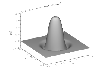
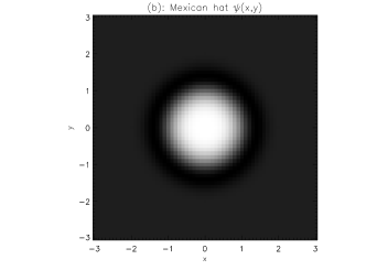
Figure 1.: Mexican hat mother wavelet, as a (a) surface and (b) contour plot. Interpreting the greyscale as opposite polarity flux, the single Mexican hat central flux concentration has a ring of opposite polarity flux. These features are also evident in the transform at all length-scales.

The continuous wavelet transform of a two-dimensional image $S$ in the domain $D\subset R^{2}$ is

$$W(L,\underline{x}^{\prime})=\int_{D}\frac{1}{L}\psi\left(\frac{\underline{x}-\underline{x}^{\prime}}{L}\right)S(\underline{x})d\underline{x}$$ (1)

where $L$ is the wavelet scale and $\underline{x}^{\prime}$ translates the wavelet across the domain $D$. The Mexican hat wavelet transform is continuous, and is implemented via the mother wavelet

$$\psi(\underline{x})=c(2-|\underline{x}|^{2})\exp\left(-|\underline{x}|^{2}/2\right)$$ (2)

for some normalization constant $c$. A plot of this mother wavelet is shown in Figure 1 (this wavelet is also used in the analysis of hewett). The wavelet is isotropic, non-orthogonal, and is a good approximation to the shapes found in active region magnetic fields.

3.2 Multiresolution median transform

As noted above, the wavelet transforms used above are good at identifying point and approximately circular features in images, but have the unfortunate side effect of introducing a “ringing” which appears as a false opposite polarity flux in the transform (Figure 1, Figure 3(I:c-h); the same effect is also clearly visible in Hewett et al. 2007). It is clearly desirable to have a transform in which positive (negative) structure in the image does not create negative (positive) structure in the transform. One such transform which has this property is the multiresolution median transform, based on the median filter.

The median transform for an image $S$ at length-scale $L$ (denoted by $\mbox{med}(S,L)$) is found by sliding a kernel of dimensions $L\times L$ at all points in the image and calculating the median value of the $L\times L$ subimage extracted from $S$. The multiresolution median transform on $N_{l}$ (specified by the user) length-scales is found by through the following algorithm:

1. Let $c_{j}=S$ with $j=1$.

2. Determine $c_{j+1}=\mbox{med}(S,2l+1)$.

3. The multiresolution coefficients $w_{j+1}$ are defined as: $w_{j+1}=c_{j}-c_{j+1}$ .

4. Let $j\leftarrow j+1$; $l\leftarrow 2l$. Return to step 2 if $j<N_{l}$ .

The original image $S$ may be reconstructed by $S=c_{N_{l}}+\sum_{j=1}^{N_{l}}w_{j}$ where $c_{N_{l}}$ is the residual image left after exiting the algorithm. In step 4, the set of resolution levels associated with $S$ lead to a dyadic decomposition. A useful feature of the median transform for analysis of active regions is that the shapes of structures on the analyzed length-scales are closer to those of the input image than would be case with a wavelet transform. The multiresolution median transform acts like a median filter operating on multiple length-scales. [Gonzalez and Woods (2001)] state that the median filter forces neighboring pixels to become more like their neighbors. This operation will preserve the structure of the field, whilst ignoring noisy outliers that may skew wavelet based processing.

3.3 An algorithm to define a Multi-scale opposite polarity region separator (MOPRS)

Algorithm “MOPRS”
1 be	gin
2	R	emove noise in image $S$ thresholding: pixels where $|B|<50$
		are set to zero.
3	D	ecompose $S$ by multiresolution transform onto $n$ length-scales, $L_{i}$
		to get transforms $W_{i}$, $1\leq i\leq n$.
4	for	i in range 1,n
5		Find zero contours in $W_{i}$
6		K	eep pixel $p_{i,a,b}$ on the zero contour if there exists opposite
			polarity fields within a 3x3 box centred on that pixel.
			in the original image $S$.
7		Report the locations of all the lines at found at this length-scale- $M_{i}$
8		Calculate the local transform power around each line in $M_{i}$.
9	end
10 end

Figure 2.: Algorithm to find Multi-scale Opposite Polarity Region Separators (MOPRS).

At a given length-scale, the wavelet transforms decompose the active region into objects of the same length-scale (Figures 3(I:a-j). The multiresolution median transform is slightly different in that the active region field structure is not directly compared to a given shape; rather, the multiresolution coefficients arise from the distribution of magnitudes of active region fluxes in the analysis window (note however that the shape of window used to define the local data at that length-scale is square.)

The organization of the active region at different scale sizes and different polarities is apparent. This makes it possible to find lines slicing the active region structure between opposing polarity regions of a given scale size. These lines are termed multi-scale opposite polarity region separators (MOPRS), and they delineate the organization of opposite polarity regions in the active region. The algorithm describing the generation of MOPRS is given in Figure 2. These lines are geometrical constructions based on the multiresolution analysis used, and since the transforms we are using are different, we can expect the MOPRS defined to vary.

The MOPRS are used to sample the gradient of the magnetic flux between regions of opposite polarity flux, at multiple length-scale, using the following algorithm.

1. Rank all the MOPRS-lines by local transform power, regardless of scale.

2. Create a mask by overlaying lines with larger local transform power over lines with smaller local transform power. This enables overlapping MOPRS with stronger local wavelet power to be preferentially represented, since MOPRS with weaker local wavelet power are replaced. Each MOPRS carries a label with the length-scale it was found at.

3. Return gradient of original image $S$ at each point on the remaining MOPRS, and assign that gradient to the MOPRS’s length-scale label.

Regardless of which multiresolution transform is used, the MOPRS exist to sample the same underlying magnetic field gradients, and so each multiresolution transform is analyzing the same complex, physical object. Different multiresolution transforms will give different samples of the same underlying magnetic field gradient, and the results obtained have to be interpreted with respect to the properties of the transform in mind. However, this is the case for all decompositions. For example, one can decompose any one dimensional time series signal using any orthogonal set; using Hermite polynomials is mathematically equivalent to using the more familiar sinusoids, and the scale content of the signal can be assessed. However, the advantage of sinusoids is that they are also the normal modes of vibration for a number of different systems, and therefore have an additional meaning on top of their convenience in understanding the scale structure of a time series. It is possible to understand the scale structure of a one dimensional time series with Hermite polynomials, but more difficult. Unfortunately, there is little or no extra guidance in choosing which multiresolution decomposition will be the “best” for understanding the complex structure of active regions, other than looking for mother wavelets that represent the object we are looking at. Therefore, in lieu of a “best possible choice”, we instead use multiple multiresolution transforms.

Figure 3(I) implements the Mexican hat transform and MOPRS analysis for some test data. Figures 3(I:a) shows the test data, whilst (I:b) shows the gradient of the image. Figures 3(I) show the Mexican hat wavelet transform of the original image at multiple length-scales. Overplotted in color are the MOPRS found at that length-scale, along with the rank of each line. These lines are then plotted on the original image and the gradient image, Figures 3(I:c,d). Discussion of the transformed images and the concomitant gradient distributions are presented below.

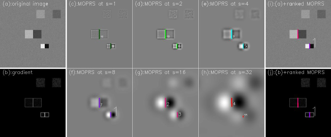
(I)

(II)

Figure 3.: Panels (I): an example MOPRS analysis using the Morlet wavelet (Section 3.1). Panel I(a) shows some test data, I(b) the magnitude of the gradient, and I(i), I(j) show I(a), I(b), respectively with MOPRS overlaid. Panels I(c-h) show the wavelet transform of test data at length-scale $s$, with the MOPRS found at that length-scale. Each line is labeled with its local wavelet power rank. Panels (ii): the same data is analyzed by the median transform. Panels II(a,b,i,j) have the same meaning as panels I(a,b,i,j). Panels II(c-h) show the median transform of the test data at length-scale $s$, with the MOPRS found at that length-scale. Each line is labeled with its local median transform power rank.

4 Results

The multiresolution analysis described above generates a large amount of information for each active region. Gradient information found along the MOPRSs measures the distribution of gradients in the line-of-sight magnetic field as a function of the length-scale of opposite polarity regions in active regions. Summary statistics of the gradient distributions (after grouping these according to Mt. Wilson class, flaring activity and length-scale) are discussed below, for the 9757 active region observations described in Section 2.

The discussion begins with examining the behaviors of the transforms themselves.

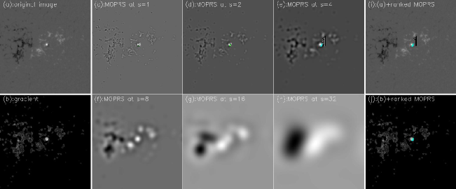
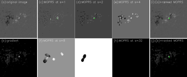
(I)

(II)

Figure 4.: Comparison of Mexican hat and median transform MOPRS for an $\alpha$ region (NOAA AR 7995, 1996/11/14 12:51 UT). See Figure 3 for a description of the ordering of the plots. A blank plot denotes that no information was found at that scale. The region is very simple, and only a very few pixels are retained as MOPRS in the median transform compared to the Mexican hat results.

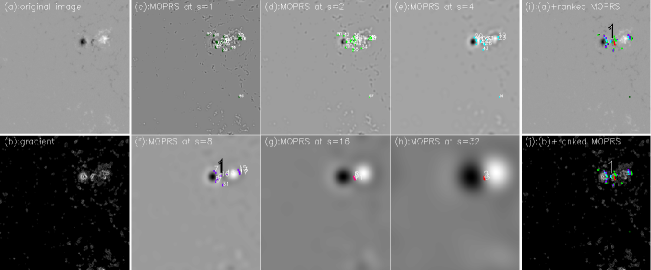
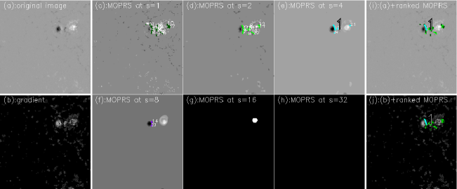
(I)

(II)

Figure 5.: Comparison of Mexican hat and median transform MOPRS for a $\beta\gamma\delta$ region (NOAA AR 2004/02/10 12:51 UT). The left two columns are Mexican Hat results, the right two columns are median transform results. The individual plots for each type transform are (a) original magnetogram, (b) original magnetogram overplotted with MOPRS from all length-scales, (c-h) multiresolution transforms at length-scales L=1,2,4,8,16 and 32 pixels respectively, overplotted with MOPRS found at that scale. Note that the thickness of the MOPRS are weighted by the local magnetic flux gradient found at that location. Both transforms capture the location of opposing polarities at small scales quite well. The Mexican hat transform appears to slice the large scale structure of the region better than the median transform.

4.1 Comparative behaviour of the transforms

It is apparent from the example transforms given in Figures 3, 4 and 5 that each transform captures different information about the active region. For example, at large scales, Figures 3(I:g,h) and 4(I:g,h) divide the plane into approximately two regions of opposite polarity, capturing the large scale distribution of the field (Figure 3(I:a), 4(I:a)). The median transform does not return any structure at the largest scale size (Figure 3(II:h), 4(II:h)). The “ringing” of the Mexican hat transform is also apparent in Figures 3(I:c-h), brought about by the shape of the transform (Section 3.1). Both multiresolution analyses report MOPRS where one would expect them, but give them different rankings. In particular, the highest ranked MOPRS occurs at different (and neighboring length-scales), but at the same location.

The median transform is much more localized, and so even although it does also find MOPRS at larger length-scales, the pixels retained as having significant gradients are far fewer. This is due to the interaction of the MOPRS algorithm (Figure 2) with the properties of the transform. The median transform cleaves more closely to the true shape of the regions [Starck, Murtagh, and Bijaoui (1998)] at that length-scale, whereas the Mexican hat transform imposes a shape on the active region. As very large scale contiguous features are not very common in active regions, they are not there for the median transform to find, and so MOPRS at these length-scales are deprecated compared to the Mexican hat transform. This is apparent in Figure 5(II:g,h), where the large scale organization of the field is found via the Mexican hat transform because the transform at that scale is smoothing out the original data over a large length-scale. This is analogous to the situation in Morlet wavelet time series analysis, where a spike (delta function) in the time series can leads to power at larger scales, even although there is no real variation at those longer scales in the data [De Moortel, Munday, and Hood (2004)]. The median transform does not detect any information at this length-scale (Figure 5(II:g,h).

Line 5 in the MOPRS algorithm (Figure 2) looks for zero contours in the transform, and so can be susceptible to the ringing effect of the Mexican hat transform. This effect is suppressed by line 6 of the MOPRS algorithm, by referring back to the original data to look for pixels on the MOPRS which do have some opposite polarity flux around them. The overall result is that the Mexican hat transform is quite effective at dividing the active region into intuitively satisfying regions, at a given length-scale. The median transform is more effective at retaining the local shape of opposite polarity regions at a given length-scale, and hence more effective at describing where opposite polarity flux is at close proximity. The MOPRS ranking algorithm also reports the most “important” MOPRS at different length-scale (Figures 3, 5). This is not very surprising, as the two multiresolution transforms are measuring very different properties of the structure. In general, it is found that the median transform assigns MOPRS to smaller length-scale than the Mexican hat transform, consistent with the behavior noted by 1998ipda.book…..S. The results quoted below from each method are consistent as a function of length-scale, as defined by each analysis method. Since the results are qualitatively the same for each method, this confirms that each method is indeed internally consistent, and both are measuring the same property of the active region field.

4.2 Gradients along MOPRS

Figure 6.: Measurements of the gradient statistics as a function of multi-resolution transform (Mexican hat, a-c; median transform, d-f), Mt. Wilson classification ($\alpha$, solid line style; $\beta$, dotted; $\beta\gamma$, dashed; $\beta\gamma\delta$, dot- dashed) and MOPRS length-scale(thick lines with plot symbols). Plots (a,d) show the average maximum gradient found on each MOPRS; plots (b,e) show the average average gradient on each MOPRS and plots (c,f) show the average standard deviation of the gradient found on each MOPRS. Also indicated are the total number of images that have at least one MOPRS at any length-scale and return a valid gradient measurement, as a function of Mt. Wilson classification (thin lines, same line style as the Mt. Wilson classification, numbers on left hand plot axis). These can vary per plot since occasionally the analysis will find a MOPRS that will return a gradient statistic which is undefined: for example, occasionally the MOPRS consists of a single point - in such a case the standard deviation of the gradient underlying this point is undefined and so must be excluded from further analysis. See Section 4.2 for more discussion of this result.

Figure 6(a-c,d-f) shows the results of measuring the gradients along the MOPRS for the active region data set for the Mexican hat and median transforms respectively. Four different statistics are returned; (a,d), maximum gradient found along the MOPRS  (b,e), average gradient found along the MOPRS  (c,f), standard deviation of the gradient along the MOPRSİn all cases, the average value of the quantity is plotted as a function of length-scale and Mt. Wilson class (gradients across the MOPRS are measured in arbitrary units).

Figure 6(a) is indicative of the other plots in this figure, regardless of the transform used. Over all length-scales, the $\beta\gamma\delta$-class has larger average maximum gradients than the $\beta\gamma$-class, which is larger than the $\beta$-class, which is larger than the $\alpha$-class (excepting where low numbers of results mean that good averages cannot be obtained). The same ordering holds for all other plots. Hence when an active region moves from one class to another, on average, the change in the geometrical structure of the active region is reflected by a change in gradient content at all length-scales, and not on any particular length-scale. All measures of the gradient given here exhibit the same property - gradients in active region classes regarded as being more likely to flare have larger maximum gradients, larger average gradients, and larger standard deviations along the MOPRS. Figures 6(c,f) suggest a greater variability in the more active classes, and so suggest that more active classes exhibit a wider range of gradient conditions, again, at all length-scales. This indicates that on average, the gradient content between opposite polarity regions maintains the same Mt. Wilson classification order, regardless of whether the field is understood as being organized on small scales, or large scales.

4.3 Weighted length-scale versus weighted gradients

  

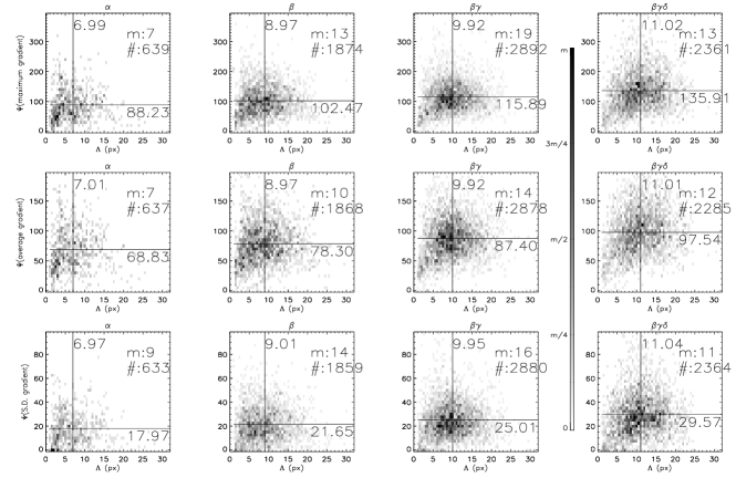
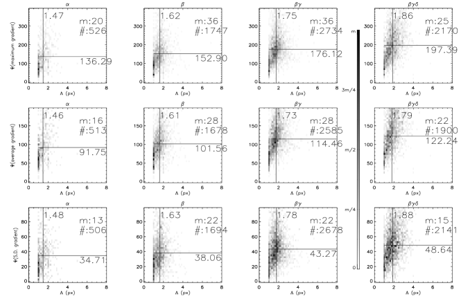
(I): Mexican hat

(II): median transform

Figure 7.: Weighted average length-scale ($\Lambda$) versus weighted average gradient statistic ($\Psi$(maximum gradient),$\Psi$(average gradient) and $\Psi$(standard deviation of gradient) ). Horizontal/vertical lines are annotated with the weighted average gradient/length-scale of the distribution. Also indicated on each plot is the maximum number of counts in a single histogram bin (’m’) and the total number of counts in the distribution (’#’). See Section 4.3 for more details on the calculation of weighted averages.

The previous results show that active region fields may on average, be ordered by Mt. Wilson classification without regard to any given length-scale. The above study also shows that gradients exist between objects of many different length-scale (active region fields are known to be multi-fractal: conlon; 2005SoPh..228….5G; 1996ApJ…465..425L; 1993ApJ…417..805L ). However, a representative length-scales and gradient statistic can be defined for a given active region, which summarizes the multiresolution nature of the active region. Assume that the MOPRS $q_{i}$ is found at length-scale $L_{q_{i}}$ and has gradient statistic (either a maximum, average or standard deviation of gradient) $G_{q_{i}}$. Further, the local wavelet power around $q_{i}$ is $w_{q_{i}}$. If there are $n$ MOPRSs, $1\leq i\leq n$ for a given active region then the weighted average MOPRS length-scale is

$$\Lambda=\sum_{i=1}^{n}w_{q_{i}}{L_{q_{i}}}/\sum_{i=1}^{n}w_{q_{i}}$$ (3)

and similarly, the weighted average gradient statistic is

$$\Psi=\sum_{i=1}^{n}w_{q_{i}}{G_{q_{i}}}/\sum_{i=1}^{n}w_{q_{i}}.$$ (4)

Weighting by the local wavelet power (the same local wavelet power of Section 3.3) takes into account the “importance” of the MOPRS found at that location.

Figure 7 plots frequency distributions of $\Lambda$ and $\Psi$ for both multiresolution analyses, for all 9757 magnetograms, binned by Mt. Wilson classification. Although the distributions are highly scattered, it is clear that in all measures, and for both multiresolution analyses, that average values of $\Lambda$ and $\Psi$ increase in the order $\alpha$$\rightarrow$$\beta$$\rightarrow$$\beta\gamma$$\rightarrow$$\beta\gamma\delta$. As the Mt. Wilson classification increases in the above order, the organization of the MOPRS moves to progressively longer length-scale, and the gradient on these separators also increases. Hence there are longer separators, with larger gradients, as the Mt. Wilson class increases to those known to have a greater chance of activity. The order $\alpha$$\rightarrow$$\beta$$\rightarrow$$\beta\gamma$$\rightarrow$$\beta\gamma\delta$ also generally connotes an increase in active region size. However, an increasing size does not necessarily mean that there are longer MOPRS between opposite polarity flux regions on those longer length-scale; it depends entirely on the locations and proximity of the opposite polarity field as it emerges. For a given size, a $\beta\gamma\delta$ active region has much more opposite polarity structure than other Mt. Wilson classes (indeed, it is implicit in the definitions - see Table 1), and so the increase in $\Lambda$ and all three $\Psi$ statistics (maximum gradient on a MOPRS, average gradient on a MOPRS, and the standard deviation of the gradient on a MOPRS), indicate the presence of increasingly diverse field structure. The qualitative result is the same for both the multiresolution results, indicating that both analyses are capturing consistent behavior.

4.4 Gradients in flaring and non-flaring active regions

  

(I): Mexican hat

(II): median transform

Figure 8.: Distributions of the maximum gradient found as a function of multi-resolution transform, analyzing gradient and flare occurence (only those flares that occur no later than six hours after the active region gradient measurement are included). In all plots, the dotted lines refer to active regions having no flares occuring in them. The thin solid line refers to active regions having at least one flare of class ’A’ or above (all-flare distribution); the thick solid line refers to active regions having class ’M’ or above (large-flare distribution). Vertical lines without asterisks indicate the mean value of the gradient distribution; vertical lines with asterisks indicate the median value of the gradient distribution. The quantity $\theta$ is the test quantity calculated to apply the Kolmogorov-Smirnov test. It is applied to test if the all-flare and large-flare distributions are different; values above 1.36 confirm the null hypothesis (that the two distributions are drawn from the same underlying distribution) less than 5% of the time - see Section 4.4 for more detail.

As suggested in the introduction, field gradients have long been associated with flaring activity. In this study, active regions are split into three sets in order to quantify the relationship between the presence of gradients between opposite polarity of different size scales and the occurance and size of flares. The first set of active regions have no flaring activity associated with them at any time. The second set of magnetograms (the all-flare set) have at least one GOES ’A1.0’ class flare, or more energetic, occuring no more than six hours after the active region magnetogram. The third set of magnetograms (the large flare set ) have at least a cumulative flare index equivalent to a GOES ’M1.0’ class flare, or more energetic, ocurring no more than six hours after the active region magnetogram. MOPRS for these magnetograms are calculated, and distributions of the maximum gradients found are shown in Figure 8.

It is clear that, on average, the gradient content of a flaring active region field is very different from that of a non-flaring active region field. Further, this difference is apparent on almost all length-scale; it does not matter which size scale one considers the opposite polarity regions to be the one at which this difference is best measured. The difference between the all-flare and large-flare distributions is less pronounced, but measurable both by looking at the mean and median values of gradients, and also by the Kolmogorov-Smirnov test. The Kolmogorov-Smirnov test for two samples (wasserman; keeping; barlow) treats the agreement between two cumulative distributions $G_{1}$ and $G_{2}$ against the null hypothesis that the two distributions are samples come from the same underlying distribution function. The first step is to calculate

$$d=\max\left|G_{1}(x)-G_{2}(x)\right|.$$ (5)

If $G_{1,2}$ has $n_{1,2}$ samples then it can be shown that

$$\lim_{n_{1},n_{2}\rightarrow\infty}\mbox{prob}\left(\theta\geq\lambda\right)=2\sum_{m=1}^{\infty}(-1)^{m+1}e^{-2m^{2}\lambda^{2}}$$ (6)

where $\theta=d\sqrt{N}$ and $N=n_{1}n_{2}/(n_{1}+n_{2})$. Values of $\theta\geq 1.36$ reject the null hypothesis at greater than or equal to the 5% level, that is, on average five times out of a hundred the two cumulative distributions come from the same underlying distribution function ($\lambda=1.63$ is equivalent to 1%, $\lambda=1.73$, 0.5% and $\lambda=1.95$, 0.1%). It is a nonparametric test and is thus appropriate to use in this case where the true gradient distribution is unknown.

The Kolmogorov-Smirnov test shows that the Mexican hat derived distributions for all-flare and large-flare maximum gradients, reject the null hypothesis with a high degree of confidence, for all the length-scale studied. The median transform results also reject the null hypothesis with a high degree of confidence, but only for the first four length-scales - the hull hypothesis cannot be rejected at length-scale= 16 and 32 pixels (probably due to insufficient data at these length-scale - see Sections 3.2 and 4.1). Hence the difference between active regions that contain any type of flare, and active regions that contain large flares is measureable in the active region gradient content, without regard to which opposite polarity region length-scale is considered.

5 Conclusions

Active region magnetic fields are known to exhibit multi-fractal properties. The study presented here connects the geometrical arrangement of opposite polarity regions (via the MOPRS concept) to the length-scale properties of the field. There appears to be no special length-scale that determines the gradient content of the active region field, which agrees with the notion from previous fractal and multi-fractal studies that there is no preferred length-scale to the spatial size of the absolute valoe of active region flux elements.

The Mt. Wilson classification does capture some structure information on the field, and through that, gradient content (Figures 6 and 7). The Mt. Wilson classification is based on the very largest length-scale describing the geometrical arrangement of the field. Figure 6 shows that regardless of the length-scale used, the gradient content of different classes of active region field can be distinguished on average. This is a result of the multi-scale nature of the active region magnetic field. Figure 7 shows that even although all Mt. Wilson classes retain their multi-scale structure (i.e., gradients at all length-scale are present), there is a general increase in the average length-scale and gradient as a function of Mt. Wilson class, in the order $\alpha$$\rightarrow$$\beta$$\rightarrow$$\beta\gamma$$\rightarrow$$\beta\gamma\delta$). Not only is the active region field appearing at larger length-scale, the organization of its gradients is also appearing at larger length-scale, and those gradients are getting larger.

The equivalence of all length-scales in the active region magnetic field is also shown in Figure 8; at all length-scale, there are measurable differences in the gradient content for active regions that give rise to large flares, active regions that give rise to all sizes of flares, and active regions that do not have flares. On average, one can distinguish the difference between these types of active region by considering the geometrical arrangement of the opposite polarity flux at any length-scale. The geometrical arrangement of opposite polarity field preserves the multi-scale nature of the active region at all length-scale, through to the gradient content of the field.

When an active region breaks through the photosphere, injection happens at multiple length-scales. The largest gradients between opposite polarity regions are observed at the smallest length-scale (see Figure 6(a,d)). Although the largest gradients may be at the smallest length-scales, gradients also exist between opposite polarity regions of longer length-scale. This study suggests that indicators of flare activity and Mt. Wilson classification exist at all length-scales, and that all active regions length-scale are equivalent, due to the multi-scale properties of the field.

Acknowledgements

This work was supported by NASA Living With a Star Targeted Research and Technology award NNH04CC65C. SOHO is a joint project of international co-operation by ESA and NASA.

References

- Abramenko (2005) Abramenko, V.I.: 2005, Multifractal Analysis Of Solar Magnetograms. Sol. Phys. 228, 29 – 42. doi:10.1007/s11207-005-3525-9.
- Abramenko et al. (2002) Abramenko, V.I., Yurchyshyn, V.B., Wang, H., Spirock, T.J., Goode, P.R.: 2002, Scaling Behavior of Structure Functions of the Longitudinal Magnetic Field in Active Regions on the Sun. ApJ 577, 487 – 495. doi:10.1086/342169.
- Barlow (1989) Barlow, R.J.: 1989, Statistics: A guide to the use of statistical methods in the physical sciences. John Wiley and Sons.
- Bratsolis and Sigelle (1998) Bratsolis, E., Sigelle, M.: 1998, Solar image segmentation by use of mean field fast annealing. A&AS 131, 371 – 375.
- Conlon et al. (2007) Conlon, P.A., Gallagher, P.T., McAteer, R.T.J., Ireland, J., Young, C.A., Kestener, P., Hewett, R., Maguire, K.: 2007, Multifractal properties of sunspot magnetic fields . Sol. Phys., this volume.
- Cui et al. (2006) Cui, Y., Li, R., Zhang, L., He, Y., Wang, H.: 2006, Correlation between solar flare productivity and photospheric magnetic field properties 1. Maximum Horizontal Gradient, Length of Neutral Line, Number of Singular Points. Sol. Phys. 237, 45 – 659. doi:10.1007/s11207-006-0077-6.
- De Moortel, Munday, and Hood (2004) De Moortel, I., Munday, S.A., Hood, A.W.: 2004, Wavelet Analysis: the effect of varying basic wavelet parameters. Sol. Phys. 222, 203 – 228. doi:10.1023/B:SOLA.0000043578.01201.2d.
- de Wit (2006) de Wit, T.D.: 2006, Fast Segmentation of Solar Extreme Ultraviolet Images. Sol. Phys. 239, 519 – 530. doi:10.1007/s11207-006-0140-3.
- Domingo, Fleck, and Poland (1995) Domingo, V., Fleck, B., Poland, A.I.: 1995, The SOHO Mission: an Overview. Sol. Phys. 162, 1 – 37.
- Falconer, Moore, and Gary (2002) Falconer, D.A., Moore, R.L., Gary, G.A.: 2002, Correlation of the Coronal Mass Ejection Productivity of Solar Active Regions with Measures of Their Global Nonpotentiality from Vector Magnetograms: Baseline Results. ApJ 569, 1016 – 1025. doi:10.1086/339161.
- Falconer, Moore, and Gary (2006) Falconer, D.A., Moore, R.L., Gary, G.A.: 2006, Magnetic Causes of Solar Coronal Mass Ejections: Dominance of the Free Magnetic Energy over the Magnetic Twist Alone. ApJ 644, 1258 – 1272. doi:10.1086/503699.
- Falconer et al. (1997) Falconer, D.A., Moore, R.L., Porter, J.G., Gary, G.A., Shimizu, T.: 1997, Neutral-Line Magnetic Shear and Enhanced Coronal Heating in Solar Active Regions. ApJ 482, 519 – +. doi:10.1086/304114.
- Gallagher, Moon, and Wang (2002) Gallagher, P.T., Moon, Y.J., Wang, H.: 2002, Active-Region Monitoring and Flare Forecasting I. Data Processing and First Results. Sol. Phys. 209, 171 – 183. doi:10.1023/A:1020950221179.
- Georgoulis (2005) Georgoulis, M.K.: 2005, Turbulence In The Solar Atmosphere: Manifestations And Diagnostics Via Solar Image Processing. Sol. Phys. 228, 5 – 27. doi:10.1007/s11207-005-2513-4.
- Gonzalez and Woods (2001) Gonzalez, R.C., Woods, R.E.: 2001, Digital image processing. Addison-Wesley Longman Publishing Co., Inc., Boston, MA, USA. ISBN 0201180758.
- Hewett et al. (2007) Hewett, R.J., Gallagher, P.T., McAteer, R.T.J., Young, C.A., Ireland, J., Conlon, P.A., Maguire, K.: 2007, A technique for multiscale analysis of turbulence in active regions using wavelets. Sol. Phys., this volume.
- Keeping (1995) Keeping, E.S.: 1995, Introdution to statistical inference (first published 1962). Dover International, Inc..
- Lawrence, Cadavid, and Ruzmaikin (1996) Lawrence, J.K., Cadavid, A.C., Ruzmaikin, A.A.: 1996, On the Multifractal Distribution of Solar Magnetic Fields. ApJ 465, 425 – +. doi:10.1086/177430.
- Lawrence, Ruzmaikin, and Cadavid (1993) Lawrence, J.K., Ruzmaikin, A.A., Cadavid, A.C.: 1993, Multifractal Measure of the Solar Magnetic Field. ApJ 417, 805 – +. doi:10.1086/173360.
- Leka and Barnes (2003a) Leka, K.D., Barnes, G.: 2003a, Photospheric Magnetic Field Properties of Flaring versus Flare-quiet Active Regions. I. Data, General Approach, and Sample Results. ApJ 595, 1277 – 1295. doi:10.1086/377511.
- Leka and Barnes (2003b) Leka, K.D., Barnes, G.: 2003b, Photospheric Magnetic Field Properties of Flaring versus Flare-quiet Active Regions. II. Discriminant Analysis. ApJ 595, 1296 – 1306. doi:10.1086/377512.
- Leka and Barnes (2007) Leka, K.D., Barnes, G.: 2007, Photospheric Magnetic Field Properties of Flaring versus Flare-quiet Active Regions. IV. A Statistically Significant Sample. ApJ 656, 1173 – 1186. doi:10.1086/510282.
- McAteer, Gallagher, and Ireland (2005) McAteer, R.T.J., Gallagher, P.T., Ireland, J.: 2005, Statistics of Active Region Complexity: A Large-Scale Fractal Dimension Survey. ApJ 631, 628 – 635. doi:10.1086/432412.
- McAteer et al. (2005) McAteer, R.T.J., Gallagher, P.T., Ireland, J., Young, C.A.: 2005, Automated Boundary-extraction And Region-growing Techniques Applied To Solar Magnetograms. Sol. Phys. 228, 55 – 66. doi:10.1007/s11207-005-4075-x.
- McIntosh (1990) McIntosh, P.S.: 1990, The classification of sunspot groups. Sol. Phys. 125, 251 – 267.
- Scherrer et al. (1995) Scherrer, P.H., Bogart, R.S., Bush, R.I., Hoeksema, J.T., Kosovichev, A.G., Schou, J., Rosenberg, W., Springer, L., Tarbell, T.D., Title, A., Wolfson, C.J., Zayer, I., MDI Engineering Team, : 1995, The Solar Oscillations Investigation - Michelson Doppler Imager. Sol. Phys. 162, 129 – 188.
- Schrijver (2007) Schrijver, C.J.: 2007, A Characteristic Magnetic Field Pattern Associated with All Major Solar Flares and Its Use in Flare Forecasting. ApJ 655, L117 – L120. doi:10.1086/511857.
- Starck, Murtagh, and Bijaoui (1998) Starck, J.L., Murtagh, F., Bijaoui, A.: 1998, Image processing and data analysis. The multiscale approach. Image processing and data analysis. The multiscale approach, Publisher: Cambridge, UK: Cambridge University Press, 1998, ISBN: 0521590841.
- Turmon, Pap, and Mukhtar (2002) Turmon, M., Pap, J.M., Mukhtar, S.: 2002, Statistical Pattern Recognition for Labeling Solar Active Regions: Application to SOHO/MDI Imagery. ApJ 568, 396 – 407. doi:10.1086/338681.
- Wall and Jenkins (2003) Wall, J.V., Jenkins, C.R.: 2003, Practical Statistics for Astronomers. Princeton Series in Astrophysics.
- Wasserman (2004) Wasserman, L.: 2004, All of statistics : A concise course in statistical inference (springer texts in statistics). Springer. ISBN 0387402721.