Predicting the species abundance distribution using a model food web

Abstract

A large number of models of the species abundance distribution (SAD) have been proposed, many of which are generically similar to the log-normal distribution, from which they are often indistinguishable when describing a given data set. Ecological data sets are necessarily incomplete samples of an ecosystem, subject to statistical noise, and cannot readily be combined to yield a closer approximation to the underlying distribution. In this paper we use empirical data obtained from an ecosystem model to study the predicted SAD in detail, resolving features which can distinguish between models but which are poorly seen in field data. We find that the power-law normal distribution is superior to both the log-normal and logit-normal distributions, and that the data can improve on even this at the high-population cut-off.

I Introduction

The species abundance distribution (SAD) is one of the most widely studied descriptions of an ecological community. To determine it, the number of species in a given community which have $n$ observed individuals is plotted against $n$. The shape of this plot has been investigated by a great many empiricists and theorists over the years, beginning with the classic work of Fisher et al. (1943) and Preston (1948). Reviews of the subject (Whittaker, 1965; May, 1975; Gray, 1987; Marquet et al., 2003; McGill et al., 2007) reveal the large number of mechanisms that have been proposed to explain the observed SAD. Many of these mechanisms predict the essential aspects of the observations, that is, a few very abundant species and many rare species. As a consequence it has become very difficult to falsify proposed mechanisms from empirical data, which has led to the authors of the most recent multi-author review (McGill et al., 2007) to contrast the development of the analysis of SADs with “a healthy scientific field” in which “theoretical, empirical and statistical developments […] advance roughly in parallel”.

In this paper we suggest a way forward which is in effect intermediate between the theoretical and empirical approaches. We measure the SAD in an established model which constructs an ecological community as a set of predator-prey interactions (Drossel et al., 2001). The model itself was originally created so that many of its key properties were emergent and not put in by hand. So, for instance, trophic levels emerge from the nature of the predator-prey interactions; species are not labelled as “plants”, “herbivores” or “carnivores” a priori. This contrasts with traditional theoretical approaches which either postulate a mechanism, or if a model community is put forward it is usually rather simple, with the form of the SAD following from one of the fundamental aspects of the theory. Conversely, measurements taken in the field will of necessity include numerous influences involving climate, terrain, location etc., which are not present in the model we use to measure SADs. Thus the SADs we measure will be free of these external influences, but still be determined by influences which are too complex to easily characterise. This approach will also allow us to measure SADs for a multi-trophic level community whereas, so far as we are aware, all other predictions for SADs have been for communities of trophically similar species.

The model we will be using (called the Webworld model) has been developed over a number of years (Caldarelli et al., 1998; Drossel et al., 2001, 2004; Quince et al., 2005). In it, species are defined in terms of traits (phenotypic and behavioural characteristics), and it is the nature of the interactions between these traits which define the nature of interactions between species. This community is built up from a small number of species through a speciation mechanism which creates a new species with a novel set of features. Resources are distributed through a quite elaborate set of equations governing population dynamics with adaptive foraging. Overviews of the model are given in review articles (Drossel & McKane, 2003; McKane & Drossel, 2005, 2006), and more briefly in section II. In section 3 we outline the method of our analysis, in section 4 we describe the results obtained and we conclude with a review of the results in section 5.

II Model description

The Webworld model consists of a set of species, each defined by its unique combination of ten different features. The features are chosen from a set of $L$ possible features determined at the start of the simulation, at which point two species are created. One of these is the environment species, which has a fixed population for all time and is the ultimate source of energy for all species in the food web. The other initial species is the common ancestor of all species encountered during a simulation run.

The dynamics of the Webworld model occur on three separated time-scales. The longest of these is the evolutionary time-scale, on which new species are added as mutated versions of extant species. Specifically to the implementation of Webworld, a species is selected at random without regard to its population, except that this must be non-zero. One individual of that species is then used to found a new species identity, sharing all features but one with the parent species. The remaining feature is selected to avoid repetition either of the same feature within one species or the same set of features between species, but is otherwise selected at random. The newly introduced species is then subject to the same population dynamics as all other species, which is the dynamical process that occurs on the intermediate time-scale.

Population dynamics occurs by balance of energy; energy is gained through “predation”, which in the case of feeding on the environment species we interpret as autotrophy. Each species $i$ changes its population $n_{i}$ according to the balance equation

$$\dot{n}_{i}=\lambda\sum_{j}g_{ij}n_{j}-\sum_{j}g_{ji}n_{i}-dn_{i},$$ (1)

where $g_{ij}$ is the functional response, the dependence of the rate of energy consumption by species $i$ on the population of species $j$. The factor of $\lambda=0.1$ introduces an ecological efficiency whereby the energy lost to species $j$ is greater than that gained by its predator $i$. Thus the first term on the right hand side of Eq. (1) is the energy income of species $i$ summed across all prey species, while the second term is the energy loss summed across all predators. If species $a$ does not feed on species $b$ then $g_{ab}=0$, and hence this does not contribute to either sum. The final term in Eq. (1) is the loss of energy from species $i$ due to death of its constituent individuals at rate $d$ per individual; the expected lifespan of an individual is therefore $1/d$, which for simplicity we take to be the same across all species. Death appears in our model purely as an energy loss term and cannot be made an evolvable quantity, since it has a preferred value of zero.

The shortest time-scale in the Webworld model reflects the choice of foraging strategy by individuals of each species. The functional response for Eq. (1) is given by

$$g_{ij}=\frac{f_{ij}S_{ij}}{bn_{j}+\sum_{k}\alpha_{ik}f_{kj}S_{kj}n_{k}}n_{i},$$ (2)

where $f_{ij}$ is the fraction of its time species $i$ spends feeding on prey species $j$, which is the quantity to be optimised in order to maximise $\sum_{j}g_{ij}n_{j}$. $S_{ij}$ and $\alpha_{ij}$ are constants defined by relating the features of species $i$ and $j$, $S$ indicating the ability of $i$ to feed on $j$, and $\alpha$ relating to the degree of inter-specific competition. To prohibit mutual predation the matrix $S$ is made anti-symmetric, thus $S_{ij}=-S_{ji}$, and the shortest possible feeding loop involves three species. Matrix $\alpha$ is symmetric, with maximum competition $\alpha_{ii}=1$ between members of the same species, and minimum competition 0.5 between highly-different species. By calculating $S$ and $\alpha$ based on a set of features largely conserved during speciation we ensure that each newly-founded species has similar abilities to its parent species, with which it is also in strong competition, and in particular the dynamics of two identical species, were they allowed, would be indistinguishable from the dynamics of pooling them as one species.

In Drossel et al. (2001) an evolutionarily stable strategy was shown to exist for foraging, which can be found by iteratively solving Eq. (2) with the condition that

$$f_{ij}=\frac{g_{ij}}{\sum_{k}g_{ik}}.$$ (3)

The result of the repeated application of these dynamics is the gradual construction of a complex food web. Species are removed if their population falls below 1, and the fixed population of the environment species, $R$, as such determines the expected number of species present in the food web at any time, though there is a continual turnover of species and consequent fluctuation in any given food web measure. After running the model for a large number of evolutionary time steps, there is no systematic change in quantities such as the number of concurrent species, and the food web structure appears to have matured. It is on such webs that we examine the species abundance distribution.

III Method

Using the Webworld model discussed in the previous section we generate sets of communities for which the ensemble species abundance distribution (SAD) can be examined in detail. Because we use the same set of possible features and the same environment species in each case, we assume that the underlying SAD does not alter between model realisations. In this case it is possible to pool the resultant communities in order to determine the SAD with improved statistical noise. Details of the computational approach are given in section III.1. In section III.2 we discuss the functions which we fit to the data, and the optimisation criteria of the fitting. In section III.3 we discuss the problems of generalising fits to include communities differing in size or trophic level.

III.1 Comparative models

Although the Webworld model can simulate ecological communities in reasonable time, to create large complex communities takes considerable computation, and to generate enough simulations to get good statistics across a broad range of parameter space is difficult. We therefore perform the first examination on a variant of Webworld in which all species feed exclusively on the environment. Because all species are basal, the relative populations are determined by the relative ability, $S$, and competition, $\alpha$, terms between existing species, which are selected by evolution in the same way as in the full model. By avoiding a large part of the computational effort we are able to generate large numbers of webs for comparison, and in the results presented here gather statistics from a set of one hundred model runs for each value of resources, $R$. In section IV we focus on the fitting of food webs with resources $10^{3}$, $10^{4}$, $10^{5}$ and $10^{6}$, but simulations were performed for numerous other values of $R$ within this range to show that interpolation of the results is reasonable. The minimum value of $R$ results in communities with few species, which become correspondingly harder to characterise in terms of an SAD. Larger values of $R$ become increasingly computationally expensive. Rather than attempting to extend the range of $R$ to larger values, we created a total of 900 basal communities at $R=10^{6}$ for more detailed analysis of the tails of the distribution. Because the common theoretical SADs have been selected based on reproduction of the modal peak, and are poorly constrained by observations, the tails offer the largest differences between candidate SADs. Due to the much larger computational complexity of the full Webworld model, we have only a sample of ten comparable food webs for large $R$ from which to deduce trophic SADs.

III.2 Fitting method

As can be seen in Figure 1, the probability distribution function (p.d.f.) of species abundance has a rather noisy histogram even for the largest collection of independent communities we were able to assemble with the available computer time. Fitting a distribution function to such histograms is problematic for several reasons. The noise makes it difficult to algorithmically optimise the fitting function, and hence can obscure differences in the strength of different functional forms. More importantly, the apparently optimal parameters and associated fitness will depend on the arbitrary choice of bin width and position, since changing these parameters can significantly alter the distribution of noise between the bins. Furthermore, the distribution function underlying the observed SAD is likely to have a functional form other than our approximations, and in general may be significantly more complicated than we can extract from data so long as the noise remains. Rather than obtaining a function which closely matches the value of the p.d.f. for most population sizes, but which omits important features, we prefer to recover a smoothed version of the distribution function which correctly predicts the total number of species. As a consequence of these considerations we fit the integrated version of the fitting function to the empirical cumulative distribution function (c.d.f.), whose value at a given population $N$ is the measured number of species with $n_{i}<N$. This definition matches the type of p.d.f. used by May (1975) whose integral is the expected number of species. P.d.f.s may also be defined such that the area enclosed is unity. To illustrate the fitting procedure we present plots of the measured and fitted c.d.f.s in addition to the p.d.f.s, and indicate the goodness-of-fit by plotting the residuals of the c.d.f., that is, the difference between the integrated fitting function and the measured c.d.f.

The strongest condition that we impose on each fitting function is that it should correctly predict the number of species more abundant than the least abundant species observed. Below this population the distribution may be terminated by a veil line, but we do not allow any such consideration for populations above the most abundant species observed. Subject to this condition we optimise the parameters of each theoretical distribution function, $f\!\left(\ln N\right)$, by minimising a quantity analogous to $\chi^{2}$. One such statistic is the Cramér-von Mises test (Bain & Engelhardt, 1991), defined as

$$CM=\frac{1}{12S}+\frac{1}{S}\sum_{i=1}^{S}\left(i-0.5-\hat{f}\!\left(n_{i}\right)\right)^{2},$$ (4)

where $\hat{f}\!\left(n_{i}\right)$ is the predicted number of species less abundant than $n_{i}$, subject to the veil line at $n_{1}$, and $S$ is the number of species observed. Although this is readily generalised to an ensemble of SADs, it attributes most weight to the peak of the distribution at the expense of fitting the tails, and we instead minimise the quantity

$$k^{2}=\int_{\ln n_{1}}^{\ln N_{\rm max}}\left(C\!\left(N\right)-\hat{f}\!\left(N\right)\right)^{2}{\rm d}\ln N,$$ (5)

where $C\!\left(N\right)$ is the observed number of species less abundant than $N$. For many distributions $N_{\rm max}\rightarrow\infty$, but functions such as the logit-normal distribution are parametrised by the total number of individuals observed, $J$, in which case $N_{\rm max}=J$. Unlike the Cramér-von Mises statistic, $k^{2}$ places equal weight in all intervals of $\ln N$. Given that the theoretical distribution almost certainly differs from the distribution underlying the data, this tends to avoid problematic regions, such as ranges of $N$ in which few species are observed, but where the empirical and theoretical c.d.f.s differ. The tails of the distribution often behave in this manner. Having identified optimal fitting parameters by minimising $k^{2}$, we follow the advice of McGill et al. (2007) that “claim[s] of a superior fit must be robust by being superior on multiple measures” by evaluating the Kolmogorov-Smirnov statistic (Hayter, 2002) for each theoretical distribution. Defined for a single realisation as

$$d=S^{-1/2}{\rm max}_{i}\left\{\left|i-1-\hat{f}\!\left(n_{i}\right)\right|,\left|i-\hat{f}\!\left(n_{i}\right)\right|\right\},$$ (6)

$d$ corresponds to the greatest deviation between the empirical and theoretical c.d.f.s. This must occur at one of the observed species, which correspond to steps in the empirical c.d.f. It is necessary to evaluate the difference between the empirical and theoretical c.d.f. both immediately before and after the step, and hence the ‘maximum’ operator in Eq. (6) contains two terms for each observation $i$. Although the values of $d$ obtained imply rejection of the theoretical distributions given the amount of data available, we use $d$ as a measure of the relative goodness-of-fit to distinguish between theoretical distributions. Other measures of goodness-of-fit tend to relate to binned data rather than the c.d.f., and provide correspondingly weaker evidence (McGill, 2003a).

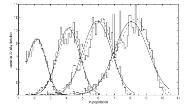
Figure 1: The fitted species abundance distribution for basal communities with resources $R=1000$, 10 000, 100 000 and 1 000 000. The histogram indicates the data in bins of width 0.1 in $\ln N$. The solid curves indicate optimal log-normal fits, the dotted lines optimal logit-normal fits, and the dashed lines optimal power-law normal fits. Distributions to the right correspond to increasing $R$.

Although the log-normal distribution has been criticised as inappropriate for application to SADs (Williamson & Gaston, 2005), it is a commonly examined form of the SAD and we therefore adopt it as one of the theoretical SADs we fit to the data. We also consider the logit-normal distribution preferred by Williamson & Gaston (2005). Whereas the log-normal distribution appears as a normal distribution when plotted against a logarithmic population-axis, the logit-normal has a normal distribution when plotted against a logit population axis. Our analysis will consistently use the logarithmic axis both for plotting and for the integration of $k^{2}$, so while the log-normal distribution has the form

$$P\!\left(\ln N\right){\rm d}\ln N=A\exp\left\{-\frac{\left(\ln N-\ln\mu\right)^{2}}{2\sigma^{2}}\right\}{\rm d}\ln N,$$ (7)

with the fitting parameters $A$, $\mu$ and $\sigma$, the logit-normal distribution includes an extra factor, giving

$$P\!\left(\ln N\right)=A\frac{J}{J-N}\exp\left\{-\frac{\left(\ln\frac{N}{J-N}-\ln\frac{\mu}{J-\mu}\right)^{2}}{2\sigma^{2}}\right\}.$$ (8)

We also consider a third fitting function, the power-law normal distribution, which appears normal against a power-law population axis. Transformed to a logarithmic axis, this has the functional form

$$P\!\left(\ln N\right)=A\alpha N^{\alpha}\exp\left\{-\frac{\left(N^{\alpha}-\mu^{\alpha}\right)^{2}}{2\sigma^{2}}\right\},$$ (9)

where $\alpha$ is the power-law index. We do not consider the log-series distribution since our data are with few exceptions peaked at large $N$, whereas the p.d.f. of the log-series distribution decreases from $N=1$ even when drawn against a logarithmic population-axis. The broken stick distribution (Magurran, 1988) was found to be similar in form to the observed distribution, but inferior to the log-normal in all cases.

III.3 Comparison of food webs

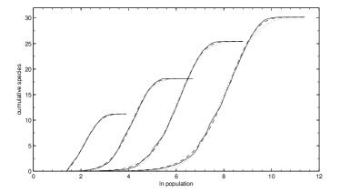
Figure 2: The fitted cumulative species abundance distribution for basal communities with resources $R=1000$, 10 000, 100 000 and 1 000 000. The solid line shows the data, the dotted line marks the log-normal distribution, and the dashed line the power-law normal distribution. Distributions to the right correspond to increasing $R$.

Since we are applying the same distribution function with different parameters to basal food webs of different sizes, and to the SADs of different trophic levels within a single community, in the ideal case a parametrisation of the fitting coefficients in terms of resources, $R$, and trophic level, $l$, would be found. Because small values of $R$ correspond to food webs with fewer species, complications arise in weighting the contribution to goodness-of-fit from differently sized webs, and we do not in this paper attempt to simultaneously fit webs of different sizes. By examination of the best-fitting parameters for each web we can determine the dependence of parameters on $R$ except in one case; the power-law index $\alpha$ of the power-law normal distribution. For most values of $R$ the goodness-of-fit depends quite weakly on this parameter, and the optimal value of $\alpha$ is poorly constrained for any one web. Since we were unable to identify a systematic trend or strongly constrain the value of $\alpha$, we chose $\alpha=0.2$ as a constant value consistent with the optimised parameters, and fixed this value for all results presented here.

IV Results

In section IV.1 we present the results of the fitting procedure for the basal communities. These should give the least complicated species abundance distributions (SADs), since all species feed on a single resource and are in direct competition with each other. In comparison, the trophic communities examined in section IV.2 feed on multiple food sources themselves distributed in abundance, and compete with different subsets of the other species. In section IV.3 we make use of the large number of simulation runs which can be performed to make a detailed examination of the low- and high-population tails of the empirical distribution, and compare this to the behaviour of the fitted distributions.

IV.1 Basal community

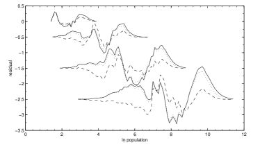
Figure 3: The same data plotted in Figure 2 shown as residuals; the solid line corresponds to the empirical c.d.f. minus the log-normal distribution, the dotted line to the data minus the logit-normal distribution, and the dashed line to the data minus the power-law normal distribution. Offsets of -0.5, -1.5 and -2.5 have been applied to data for resources $R=10\,000$, 100 000 and 1 000 000 respectively.

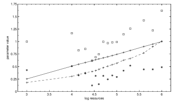
Figure 4: Parameters of the power-law normal fit to the basal community SAD for all values of resources examined. The solid line passes through points marking the mean population, $\mu$ in Eq. (9); the dashed line marks the standard deviation, $\sigma$. Squares mark the Kolmogorov-Smirnov $d$ value, and stars mark the quantity $K$ described in the text.

The results for this version of the model are the most complete in that one hundred simulations runs were examined for each value of resources $R$, and a large number of values of the continuous parameter were examined. In Figures 1 to 3 only four of these realisations are plotted, corresponding to $R=10^{3}$, $10^{4}$, $10^{5}$ and $10^{6}$, which include the two most extreme values of $R$ for which webs were calculated. The general features of the SAD for these four values are typical, as is the goodness of fit achieved by each of the three fitting functions examined. It is clear from Figure 1 that the observed distribution is left-skewed (has an over-abundance of rarer species), a characteristic absent from the log-normal distribution. The logit-normal distribution does not have significantly improved skew over the log-normal distribution, since the most abundant species from any run has less than one quarter of the mean number of individuals $J$, and the logit function is therefore well below its asymptotic cut-off. Williamson & Gaston (2005) note that in this limit the logit-normal distribution approaches the log-normal. The power-law normal distribution much more closely captures the smaller high-$N$ tail. The corresponding cumulative distribution functions (c.d.f.s) are plotted in Figure 2, where the logit-normal distribution has been omitted for clarity. It can be seen, especially for $R=10^{6}$, that the log-normal distribution underestimates the cumulative number of species in both tails, which corresponds to the skew of the p.d.f., and that even for one hundred realisations the empirical c.d.f. is far from smooth. More instructive than the c.d.f. are the residuals of this plot, that is, the difference between the instantaneous value of the empirical c.d.f. and the fitting function. These are shown in Figure 3 for all three fitting functions. The integral of the square of this plot is our goodness-of-fit measure $k^{2}$, and the maximum deviation from zero is the Kolmogorov-Smirnov $d$-measure. Substantial structure can be seen in the residuals, especially the central peak for each value of $R$ when examining the power-law normal distribution, which most closely mimics the tails. Table 1 records the values of $k^{2}$ and the Kolmogorov-Smirnov $d$ value for each fit, for fitting parameters minimising $k^{2}$. Basal communities are labelled by the value of resources, $R$, while trophic levels examined in section IV.2 are labelled according to the trophic level, $l$. For the basal food webs the power-law normal fit always outperforms both the logit-normal and log-normal distributions in terms of $k^{2}$, and is only in one case inferior to the logit-normal distribution as measured by $d$. A further comparison of the relative merits of the theoretical distribution functions is given in section IV.3.

In Figure 4 we plot the dependence of the parameters of the power-law normal fit on $R$, as well as the two goodness-of-fit indicators used. The solid line, marking the population of the peak of the distribution, indicates the very near linearity of the value of the peak of the distribution with $\ln R$. The standard deviation of the distribution increases more rapidly than linearly, as indicated by the dashed line. The value of $k^{2}$ increases with $\ln R$ for two reasons. Firstly, it is measured on the full c.d.f. rather than the normalised distribution, and so tends to increase as the square of the expected number of species, $S$. Secondly, because it is an integrated measure, it tends to increase with the width of the distribution, which we characterise by the standard deviation of the log-normal distribution, $\sigma_{\rm LN}$. It is more appropriate to use this measure than the standard deviation of the power-law normal itself since the former corresponds naturally to the width along the logarithmic population axis. In Figure 4 we plot the quantity

$$K=\frac{1000k^{2}}{S^{2}\sigma_{\rm LN}},$$ (10)

which compensates for these effects, and includes a factor of $1000$ to scale it appropriately for that plot. It can be seen that intermediate values of $R$ are the best fitted, as measured by either $K$ or the Kolmogorov-Smirnov $d$, perhaps due to relatively small amounts of additional structure.

IV.2 Trophic levels

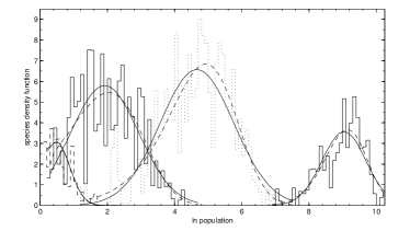
Figure 5: Histograms mark the observed species abundance distribution for the four trophic levels found in the ten Webworld communities examined. Trophic levels two and four are marked by dotted and dashed lines respectively. Solid curves mark the optimal log-normal fits to each trophic level, and dashed lines the optimal power-law normal fits.

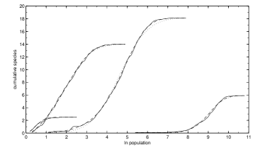
Figure 6: The cumulative species abundance distribution for Webworld communities corresponding to the four observed trophic levels. Higher trophic levels are to the left of lower levels, having smaller typical populations. Optimal log-normal fits are marked by dotted lines, and optimal power-law normal fits by dashed lines.

Having established that the power-law normal distribution describes the SAD reasonably well for basal communities, we apply it to individual trophic levels of full Webworld communities to determine the relevant fitting parameters. Due to the small number of food webs available, and the small number of species in each trophic level for any one web, it is inappropriate to seek deviations from this distribution with the data available, although we find that the power-law normal distribution is adequate, and superior in all cases to the log-normal distribution, having smaller values of both $k^{2}$ and $d$. As indicated by the values given in table 1, the logit-normal distribution marginally improves upon the power-law normal distribution for trophic levels 1 and 3, but is significantly inferior to the power-law normal for trophic level 2. For trophic level 1, the typical number of species observed per web in the data examined was only 5.9, the most abundant species being nearly half the total population of its trophic level. For trophic level 3 the lower tail of the distribution was truncated, and although here the logit-normal distribution performed better than the power-law normal, it is not clear that the logit-normal is able to adequately reproduce the whole SAD. Although four trophic levels were found in the empirical data, a very small number of species were found in trophic level 4. It can be seen in Figure 5 that the distribution function of this level is little more than the high-population tail of the distribution function, and no reliable results can be obtained by its analysis.

For comprehension of the empirical distribution being fitted we reproduce, in Figure 6, the cumulative distribution function constructed from the simulation data along with the optimal log-normal and power-law normal fits. It can be seen clearly from this figure that the distribution of the second trophic level, which has the largest number of species in total, is closest in form the those of the basal communities. The distribution of trophic level three, to its left, passes the veil line before a significant fraction of the low-population tail has been exposed, but is otherwise in good agreement with the basal community distributions. The lowest trophic level, however, seems relatively truncated, resulting in a much sharper cutoff at large $N$ than is reproduced by either the log-normal or power-law normal distributions. The cause of this may relate to the presence of predators, who can be expected to preferentially target the most abundant prey, but additional data are required to investigate this hypothesis. The residuals of the c.d.f. fits are shown in Figure 7; it is possible that similar structure in these is present to that seen for the basal communities in Figure 3, but the degree of noise is greater.

In Figure 8 the mean and standard deviation of the power-law normal distribution are plotted as a function of trophic level. While the standard deviation appears to decline linearly with trophic level, the distribution mean may decrease more slowly. However, if the results for trophic level four are misleading due to

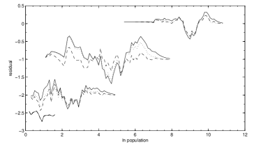
Figure 7: The same data plotted in Figure 6 shown as residuals; the solid line corresponds to the empirical c.d.f. minus the log-normal distribution, the dotted line to the data minus the logit-normal distribution, and the dashed line to the data minus the power-law normal distribution. Offsets of -1.0, -2.0 and -2.5 have been applied to data for trophic levels 2, 3 and 4 respectively. No logit-normal fit was obtained for trophic level 4 due to the absence of a positive optimal mean.

the extremely high position of the veil line, and the distribution of basal species is possibly altered through predation as discussed, the reliability of these results is limited. The quantity $K$, defined in Eq. (10), is much better for trophic levels two and three than for either the basal or fourth trophic level, although only marginal improvements in the Kolmogorov-Smirnov $d$ value can be seen.

IV.3 Distribution tails

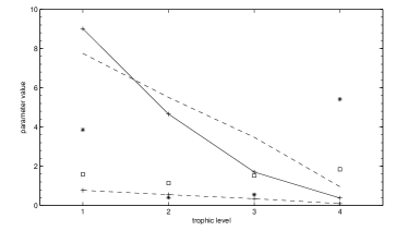
Figure 8: Parameters of the power-law normal fit to the trophic community SAD for all values of resources examined. The solid line passes through points marking the mean value of $N$. The lower dashed line marks the standard deviation, while the upper dashed line multiplies this quantity by 10 for clarity. Squares mark the Kolmogorov-Smirnov $d$ value. Stars mark the quantity $K$ defined in the text.

An advantage of examining computationally derived communities of species is that extremely large data sets can be constructed with relative ease, subject only to the availability of computer time. In addition, the Webworld model produces complete ecological communities, and the sampling effects associated with field data are avoidable. As such it is much more feasible to examine the form taken by the tails of the distribution function, which McGill et al. (2007) note are subject to noisy data, but which often contain the main differences between theoretical distributions.

To construct a high-quality empirical SAD whose tails could be examined, nine hundred simulation runs were performed for the basal community with $R=10^{6}$. The low-population tail of this distribution is plotted in Figure 9, where the logarithm of the binned species abundance has been taken to expose the tail. The fact that a linear regression to this data (not shown) produces a good fit for $\ln N<7$ implies that in this regime a power-law fit,

$$P\!\left(\ln N\right)\propto N^{a},$$ (11)

with $a\sim 4/3$, is obeyed. The power-law normal distribution is able to reproduce this form reasonably well, while both the log-normal and logit-normal distributions significantly underestimate the number of species present.

The distribution tail for large populations is shown in Figure 10. Here bins have been chosen to be uniform in width in population, rather than uniform in $\ln N$, in order to resolve the tail. The result is that a different version of the distribution is shown,

$$P\!\left(N\right){\rm d}N=\frac{P\!\left(\ln N\right)}{N}{\rm d}N,$$ (12)

which, when integrated with respect to $N$, gives the c.d.f. Note that in order to highlight the form of the decay, the population axis has been stretched to a power-law. The regression line, plotted as a dash-dot line, indicates that the high-population tail has the form

$$P\!\left(N\right){\rm d}N\propto\exp\left\{-\left(\frac{N}{7140}\right)^{1.4116}\right\}{\rm d}N.$$ (13)

As can be seen in Figure 10, this form of the decay declines more rapidly with $N$ than any of the log-normal, logit-normal or power-law normal distributions examined.

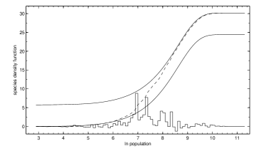
Figure 11: The c.d.f. for the basal community with resources $R=10^{6}$, as shown in Figure 2, is shown as a dashed line. The solid lines mark the c.d.f. constructed from fits to the tails as described in the text. The histogram marks the residuals of the p.d.f. of this fit.

Having established probable forms for the low- and high-population tails by regression to Figures 9 and 10, we combine these into a distribution which has the minimum value of the two tail-fitting functions for all $N$. In addition to the dashed line marking the empirical c.d.f., identical to that shown in Figure 2, this fit is shown in Figure 11 in two forms. The lower plot is the c.d.f. integrated from zero species at $N=0$, and the upper curve is integrated down from the observed number of species so as to converge with the empirical distribution at large $N$. The fact that the latter curve is above the former indicates that the combined distribution underestimates the total number of species, implying that it under-predicts the p.d.f. near the peak, to which it was not fitted. Figure 11 therefore also plots the residuals of the tail-fitting distribution as a histogram. There appear to be at least three peaks in the residuals, making it difficult to identify a plausible general form. Since we do not have unrelated basal food webs to examine, in particular to establish what parameters of the tail distributions are generic and whether the residuals show a common pattern, it is not appropriate to draw further conclusions about the central part of the distribution. We are also unable to ascribe a goodness-of-fit to the tail-based distribution due to its inability to reproduce the peak of the distribution.

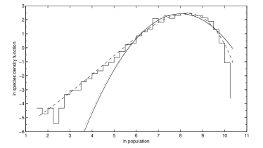
Figure 9: The small population tail of the basal community p.d.f. for resources $R=10^{6}$. The p.d.f. is described in the text. The solid, dotted and dashed curves mark the log-normal, logit-normal and power-law normal fits to Figure 2 respectively.

V Conclusions

Figure 10: The high population tail of the basal community p.d.f. for resources $R=10^{6}$. The $x$-axis is linear in $N^{1.4116}$, which was found to be the power-law index minimising the $\chi^{2}$ of the regression line, but has been marked with corresponding values of $N$ for clarity. The histogram marks the value of $P\!\left(N\right)$, the population density in bins of equal width in $N$. The solid, dotted and dashed curves mark the log-normal, logit-normal and power-law normal fits to Figure 2 respectively. The dash-dotted line indicates the best-fitting regression for $N>2000$.

We have investigated the form of the species abundance distribution empirically derived from simulation results of the Webworld food web model. This model was created to examine patterns of food web assembly, and the form of the species abundance distribution (SAD) was not a factor in its construction. Rather, the use of population dynamics to establish the success of particular species and feeding strategies within the community lead naturally to variation in the abundance of species which appears similar to the SADs identified from real ecosystems. By investigating the empirical SAD from the simulations in the same manner as data from real ecosystems we are able to characterise not only the peak of the distribution, which is frequently observed to have a form similar to the log-normal distribution, but to examine in detail parts of the distribution difficult to obtain data on from field studies. We agree with the conclusion of Williamson & Gaston (2005) that the logit-normal distribution fits better, but with particular reference to the tails of the distribution find that the power-law normal distribution function is better still. In particular, the log-normal and logit-normal distributions predict that the number of species with population $N$ falls more rapidly with decreasing $N$ than we obtain from our simulation results, which the power-law normal distribution matches very well in this tail.

The presence of structure in Figure 3 suggests that a more complicated function is needed to properly reproduce the observed SAD, but we have not been able to examine the reproducibility of this remaining structure. All the food webs examined were created for the same set of possible features and the same environment species. To fully explore the results even for a single value of $R$ would require the use of food webs constructed for ‘worlds’ with different environment species and feature sets. In undertaking such a programme it would first be necessary to establish whether such parameters as the mean and variance of the fitted distribution changed, or more generally to construct the meta-distribution of a large number of Webworld ‘worlds’ and test, using the Kolmogorov-Smirnov $d$ value, whether the empirical distribution constructed from webs of a single family was consistent with the meta-distribution.

We find that the power-law normal distribution identified as well describing the SAD of a basal community is also successful in describing individual trophic levels of a food web. It is particularly descriptive of the second trophic level, which can be seen in Figures 5 and 6 to be the most completely realised by our empirical data. The higher trophic levels can also be expected to be well-fitted by the power-law normal distribution, although the truncation of the distribution at low populations results in the log-normal and logit-normal descriptions also being adequate. The empirical distribution of the lowest trophic level is more sharply truncated at high populations than seen for other communities, the reason for which would require substantial additional investigation. Unlike the case of examining basal communities at different values of $R$, only a small number of trophic levels are ever possible, and hence the relation between them is harder to quantify. While it would be possible to construct meta-distributions from larger numbers of food webs, it is more feasible to first examine the agreement between the meta-distributions of basal communities and the constituent distributions. If there is good agreement, the agreement between the meta-distribution and the trophic distributions should be examined. If not, then a very large number of communities need to be evolved in the same environment in order to study the relation between trophic levels, potentially also examining the effect of different values of $R$. The main problem in investigating the SAD of numerically modelled ecosystems is the extensive computer time required to provide data.

The SADs constructed for this paper are complete not only in the sense that they contain all individuals present in the sample area, but also in that they do not feature immigrant or transient species, which can contribute to the low-population tail without representing a viable population. While features such as immigration from surrounding communities can easily be incorporated into our model, as can finite population effects, their exclusion demonstrates the existence of an extensive low-population tail to the distribution even for a closed ecosystem. This contrasts with the proposal by Magurran (2003) that the low-population tail is a log-series distribution of “occasional” species added to a core log-normal distribution. Although we do not agree with McGill (2003b) that left-skew is purely an effect of sampling, it may be the case that the left-skew of incomplete samples does not reflect the underlying distribution.

McGill et al. (2007) observe that most proposed SADs are similar to one another except in the tails, which is precisely the region which field observations are least able to address due to paucity of data. This issue can be addressed by the use of any model which can produce multiple independent realisations of its dynamics from which a composite SAD can be constructed, but this process can only be used to inform the analyses which should be performed on ecological data, since it is not known a priori that any given model accurately reproduces the real SAD. A virtue of the Webworld model is that is produces a plausible SAD without any such consideration having been used during the model design, being based rather on plausible ecological rules.

Table 1: Comparison of measures of goodness-of-fit for the log-normal, logit-normal and power-law normal distributions to basal community SADs and trophic SADs.

Community	Species	$k^{2}$
	$S$	Log	Logit	Power-law
$R=10^{3}$	11.22	0.0599	0.0390	0.0314
$R=10^{4}$	18.15	0.2333	0.1571	0.1175
$R=10^{5}$	25.42	0.8820	0.6296	0.1676
$R=10^{6}$	30.16	1.5759	1.1752	0.4708
$l=1$	5.9	0.1532	0.0902	0.0877
$l=2$	18.1	0.7972	0.5328	0.1480
$l=3$	14.0	0.2111	0.1126	0.1093
Community	Species	Kolmogorov-Smirnov $d$
	$S$	Log	Logit	Power-law
$R=10^{3}$	11.22	1.0648	1.1094	0.9990
$R=10^{4}$	18.15	1.3244	1.0409	1.1660
$R=10^{5}$	25.42	1.4826	1.3669	0.9919
$R=10^{6}$	30.16	2.0255	1.7661	1.6167
$l=1$	5.9	1.8391	1.5798	1.5934
$l=2$	18.1	2.0051	1.7753	1.1430
$l=3$	14.0	1.8270	1.4797	1.5241

References

- Fisher et al. (1943) Fisher, R. A., Corbet, A. S., Williams, C., 1943; The relationship between the number of species and the number of individuals in a random sample from an animal population. J. Animal Ecology 12 42
- Preston (1948) Preston, F. W., 1948; The commonness and rarity of species. Ecology 29 254
- Gray (1987) Gray, J. S., 1987; Species-abundance patterns. In Organization of Communities Past and Present (J. H. R. Gee, P. S. Giller, eds.) (Blackwell Science, Oxford), 53–68
- Marquet et al. (2003) Marquet, P. A., Fernández, J. A., Cofre, H., 2003; Breaking the stick in space: of niche models, metacommunities and patterns in the relative abundance of species. In Macroecology: Concepts and Consequences (T. M. Blackburn, K. J. Gaston, eds.) (Blackwell Science, Oxford), 64–86
- May (1975) May, R. M., 1975; Patterns of species abundance and diversity. In Ecology and evolution of communities (M. L. Cody, J. M. Diamond, eds.) (Belknap Press, Harvard), 81–120
- McGill et al. (2007) McGill, B. J., Etienne, R. S., Gray, J. S., Alonso, D., Anderson, M. J., Benecha, H. K., Dornelas, M., Enquist, B. J., Green, J. L., He, F., Hurlbert, A. H., Magurran, A. E., Marquet, P. A., Maurer, B. A., Ostling, A., Soykan, C. U., Ugland, K. I., White, E. P., 2007; Species abundance distributions: moving beyond single prediction theories to integration within an ecological framework. Ecology Letters 10 995
- Whittaker (1965) Whittaker, R. H., 1965; Dominance and diversity in land plant communities. Science 147 250
- Drossel et al. (2001) Drossel, B., Higgs, P. G., McKane, A. J., 2001; The influence of predator-prey population dynamics on the long term evolution of food web structure. J. Theor. Biol. 208 91
- Caldarelli et al. (1998) Caldarelli, G., Higgs, P. G., McKane, A. J., 1998; Modelling coevolution in multispecies communities. J. Theor. Biol. 193 345
- Drossel et al. (2004) Drossel, B., McKane, A. J., Quince, C., 2004; The impact of nonlinear functional responses on the long-term evolution of food web structure. J. Theor. Biol. 229 539
- Quince et al. (2005) Quince, C., Higgs, P. G., McKane, A. J., 2005; Topological structure and interaction strengths in model food webs. Ecol. Model. 187 389
- Drossel & McKane (2003) Drossel, B., McKane, A. J., 2003; Modelling food webs. In Handbook of Graphs and Networks (S. Bornholdt and H.G. Schuster, ed.) (Wiley-VCH), 218–247
- McKane & Drossel (2005) McKane, A. J., Drossel, B., 2005; Modelling evolving food webs. In Dynamical Food Webs (P. C. de Ruiter, V. Wolters, J. C. Moore, eds.) (Elsevier, Singapore), 74–88
- McKane & Drossel (2006) McKane, A. J., Drossel, B., 2006; Models of food web evolution. In Ecological Networks: Linking Structure to Dynamics in Food Webs (Oxford University Press), 223–243
- Bain & Engelhardt (1991) Bain, L. J., Engelhardt, M., 1991; Introduction to Probability and Mathematical Statistics (Duxbury)
- Hayter (2002) Hayter, A. J., 2002; Probability and Statistics for Engineers and Scientists (Duxbury), 2nd edn.
- McGill (2003a) McGill, B. J., 2003a; Strong and weak tests of macroecological theory. Oikos 102 679
- Williamson & Gaston (2005) Williamson, M., Gaston, K. J., 2005; The lognormal distribution is not an appropriate null hypothesis for the species adundance distribution. J. Animal Ecology 74 409
- Magurran (1988) Magurran, A. E., 1988; Ecological diversity and its measurement (Cambridge University Press)
- Magurran (2003) Magurran, A. E., 2003; Explaining the excess of rare species in natural species abundance distributions. Nature 422 714
- McGill (2003b) McGill, B. J., 2003b; Does Mother Nature really prefer rare species or are log-left-skewed SADs a sampling artefact? Ecology Letters 6 766