Acoustic cloaking theory

Abstract

An acoustic cloak envelopes an object so that sound incident from all directions passes through and around the cloak as though the object were not present. A theory of acoustic cloaking is developed using the transformation or change-of-variables method for mapping the cloaked region to a point with vanishing scattering strength. We show that the acoustical parameters in the cloak must be anisotropic: either the mass density or the mechanical stiffness or both. If the stiffness is isotropic, corresponding to a fluid with a single bulk modulus, then the inertial density must be infinite at the inner surface of the cloak. This requires an infinitely massive cloak. We show that perfect cloaking can be achieved with finite mass through the use of anisotropic stiffness. The generic class of anisotropic material required is known as a pentamode material. If the transformation deformation gradient is symmetric then the pentamode material parameters are explicit, otherwise its properties depend on a stress like tensor which satisfies a static equilibrium equation. For a given transformation mapping the material composition of the cloak is not uniquely defined, but the phase and wave speeds of the pseudo-acoustic waves in the cloak are unique. Examples are given from 2D and 3D.

1 Introduction

The observation that the electromagnetic equations remain invariant under spatial transformations is not new. Ward and Pendry [1] used it for numerical purposes, but the result was known to Post [2] who discusses it in his book, and it was probably known far earlier. The recent interest in passive cloaking and invisibility is due to the fundamental result of Greenleaf, Lassas an Uhlmann [3, 4] that singular transformations could lead to cloaking for conductivity. Not long after this important discovery, Pendry et al. [5] and Leonhardt [6] made the key observation that singular transformations could be used to achieve cloaking of electromagnetic waves. These results and others have generated significant interest in the possibility of passive acoustic cloaking.

Acoustic cloaking is considered here in the context of the so-called transformation or change-of-variables method. The transformation deforms a region in such a way that the mapping is one-to-one everywhere except at a single point, which is mapped into the cloak inner boundary, see Figure 1. The acoustic problem is for the infinitesimal pressure $p({\mbox{\boldmath$\displaystyle\mathbf{x}$}},t)$ which satisfies the scalar wave equation in the surrounding fluid,

$$\nabla^{2}p-\ddot{p}=0.$$ (1)

The basic idea is to alter the cloak’s acoustic properties (density, modulus) so that the modified wave equation in $\omega$ mimics the exterior equation (1) in the entire region $\Omega$. This is achieved if the spatial mapping of the simply connected region $\Omega$ to the multiply connected cloak $\omega$ has the property that the modified equation in $\omega$ when expressed in $\Omega$ coordinates has exactly the form of (1) at every point in $\Omega$.

Figure 1: The undeformed simply connected region $\Omega$ is transformed by the mapping $\displaystyle\mathbf{\chi}$ into the multiply connected cloak $\omega$. Essentially, a single point $\displaystyle\mathbf{O}$ is transformed into a hole (the invisible region) surrounded by the cloak $\omega$. The outer boundary $\partial\omega_{+}$ is coincident with $\partial\Omega_{+}(=\partial\Omega)$ and the inner boundary $\partial\omega_{-}$ is the image of the point $\displaystyle\mathbf{O}$. Apart from $\displaystyle\mathbf{O}$ and $\partial\omega_{-}$ the mapping is everywhere one-to-one and differentiable.

The objective here is to answer the question: What type of material is required to realize these unusual properties that make an acoustic cloak? While cloaking cannot occur if the bulk modulus and density are simultaneously scalar quantities (see below), it is possible to obtain acoustical cloaks by assuming the mass density is anisotropic [7, 8, 9]. A tensorial density is not ruled out on fundamental grounds [10] and in fact there is a strong physical basis for anisotropic inertia. For instance, Schoenberg and Sen [11] showed that the inertia tensor in a medium comprising alternating fluid constituents is transversely isotropic with elements $\langle\rho\rangle$ in the direction normal to the layering, and $\langle\rho^{-1}\rangle^{-1}$ in the transverse direction, where $\langle\cdot\rangle$ is the spatial average. Anisotropic effective density can arise from other microstructures, as discussed by Mei et al. [12] and by Torrent and Sánchez-Dehesa [13]. The general context for anisotropic inertia is the Willis equations of elastodynamics [14] which Milton et al. [10] showed are the natural counterparts of the EM equations that remain invariant under spatial transformation. Acoustic cloaking has been demonstrated, theoretically at least, in both 2D and 3D: a spherically symmetric cloak was discussed by Chen and Chan [8] and by Cummer et al. [9], while Cummer and Schurig [7] described a 2D cylindrically symmetric acoustic cloak. These papers use a linear transformation based on prior EM results in 2D [15].

Cloaks based on anisotropic density in combination with the inviscid acoustic pressure constitutive relation (bulk modulus) will be called Inertial Cloaks (IC). The fundamental mathematical identity behind the IC is the observation of Greenleaf et al. [16] that the scalar wave equation is mapped into the following form in the deformed cloak region

$$\frac{1}{\sqrt{|g|}}\frac{\partial~{}}{\partial x_{i}}\bigg{(}\sqrt{|g|}\,g^{ij}\frac{\partial p}{\partial x_{j}}\bigg{)}-\ddot{p}=0,\quad{\mbox{\boldmath$\displaystyle\mathbf{x}$}}\in\omega.$$ (2)

Here $g=(g_{ij})$ is the Riemannian metric with $|g|=\det(g_{ij})$, $(g^{ij})=(g_{ij})^{-1}$. The reader familiar with differential geometry will recognize the first term in eq. (2) as the Laplacian in curvilinear coordinates. Comparison of the transformed wave equation (2) with the IC wave equation provides explicit expressions for the IC density tensor and the bulk modulus [17].

We will derive an identity equivalent to (2) in Section 2 using an alternative formulation adapted from the theory of finite elasticity. A close examination of the anisotropic density of the IC shows that its volumetric integral, the total mass, must be infinite for perfect cloaking. This raises grave questions about the utility of the IC. The remainder of the paper provides a solution to this quandary. The main result is that the IC is a special case of a more general class of acoustic cloaks, defined by anisotropic inertia combined with anisotropic stiffness. The latter is obtained through the use of pentamode materials (PM) [18]. In the same way that an ideal acoustic fluid can be defined as the limit of an isotropic elastic solid as the shear modulus tends to zero, there is a class of limiting anisotropic solids with five (hence penta) easy modes of deformation analogous to shear, and one non-trivial mode of stress and strain. The general cloak comprising PM and IC is called the PM-IC model. The additional degrees of freedom provided by the PM-IC allow us to avoid the infinite mass dilemma of the IC.

We begin in Section 2 with a new derivation of the inertial cloak (IC) model, and a discussion of the infinite mass dilemma. Pentamode materials are introduced in Section 3 where it is shown that they display simple wave properties, such as an ellipsoidal slowness surface. The intimate connection between PM and acoustic cloaking follows from Theorem 1 in Section 4. Properties of the generalized PM-IC model for cloaking are developed in Section 4 through the use of an example cloak that can be pure IC or pure PM as a parameter is varied. Further examples are given in Section 5, with a concluding summary of the generalized acoustic cloaking theory in Section 6.

2 The inertial cloak

The transformation from $\Omega$ to $\omega$ is described by the point-wise deformation from ${\mbox{\boldmath$\displaystyle\mathbf{X}$}}\in\Omega$ to ${\mbox{\boldmath$\displaystyle\mathbf{x}$}}={\mbox{\boldmath$\displaystyle\mathbf{\chi}$}}({\mbox{\boldmath$\displaystyle\mathbf{X}$}})\in\omega$. In the language of finite elasticity, $\displaystyle\mathbf{X}$ describes a particle position in the Lagrangian or undeformed configuration, and $\displaystyle\mathbf{x}$ is particle location in the Eulerian or deformed physical state. The transformation or mapping defined by $\displaystyle\mathbf{\chi}$ is one-to-one and invertible except at the single point ${\mbox{\boldmath$\displaystyle\mathbf{X}$}}={\mbox{\boldmath$\displaystyle\mathbf{O}$}}$, see Figure 1. We use $\nabla$, $\nabla_{X}$ and $\operatorname{div}$, $\operatorname{Div}$ to indicate the gradient and divergence operators in $\displaystyle\mathbf{x}$ and $\displaystyle\mathbf{X}$, respectively. The component form of $\operatorname{div}{\bf A}$ is $\partial A_{i}/\partial x_{i}$ or $\partial A_{ij}/\partial x_{i}$ when ${\bf A}$ is a vector and a second order tensor-like quantity, respectively. The deformation gradient is defined ${\mbox{\boldmath$\displaystyle\mathbf{F}$}}=\nabla_{X}{\mbox{\boldmath$\displaystyle\mathbf{x}$}}$ with inverse ${\mbox{\boldmath$\displaystyle\mathbf{F}$}}^{-1}=\nabla{\mbox{\boldmath$\displaystyle\mathbf{X}$}}$, or in component form $F_{iI}=\partial x_{i}/\partial X_{I}$, $F_{Ii}^{-1}=\partial X_{I}/\partial x_{i}$. The Jacobian of the deformation is $J=\det{\mbox{\boldmath$\displaystyle\mathbf{F}$}}=|{\mbox{\boldmath$\displaystyle\mathbf{F}$}}|$, or in terms of volume elements in the two configurations, $J=\operatorname{d}v/\operatorname{d}V$. The polar decomposition implies ${\mbox{\boldmath$\displaystyle\mathbf{F}$}}={\mbox{\boldmath$\displaystyle\mathbf{V}$}}{\mbox{\boldmath$\displaystyle\mathbf{R}$}}$, where $\displaystyle\mathbf{R}$ is proper orthogonal (${\mbox{\boldmath$\displaystyle\mathbf{R}$}}{\mbox{\boldmath$\displaystyle\mathbf{R}$}}^{t}={\mbox{\boldmath$\displaystyle\mathbf{R}$}}^{t}{\mbox{\boldmath$\displaystyle\mathbf{R}$}}={\mbox{\boldmath$\displaystyle\mathbf{I}$}}$, $\det{\mbox{\boldmath$\displaystyle\mathbf{R}$}}=1$) and the left stretch tensor ${\mbox{\boldmath$\displaystyle\mathbf{V}$}}\in$Sym⁺ is the positive definite solution of ${\mbox{\boldmath$\displaystyle\mathbf{V}$}}^{2}={\mbox{\boldmath$\displaystyle\mathbf{F}$}}{\mbox{\boldmath$\displaystyle\mathbf{F}$}}^{t}$. The analysis is as far as possible independent of the spatial dimension $d$, although applications are restricted to $d=2$ or $d=3$.

The principal result for the inertial cloak is

Lemma 1

$$\nabla_{X}^{2}p=J\,\operatorname{div}\big{(}J^{-1}{\mbox{\boldmath$\displaystyle\mathbf{V}$}}^{2}\nabla p\big{)}.$$ (3)

Proof: The right hand side can be expressed

$$J\,\operatorname{div}\big{(}J^{-1}{\mbox{\boldmath$\displaystyle\mathbf{F}$}}{\mbox{\boldmath$\displaystyle\mathbf{F}$}}^{t}\nabla p\big{)}=JJ^{-1}({\mbox{\boldmath$\displaystyle\mathbf{F}$}}^{t}\nabla)\cdot\big{(}{\mbox{\boldmath$\displaystyle\mathbf{F}$}}^{t}\nabla p\big{)}+J({\mbox{\boldmath$\displaystyle\mathbf{F}$}}^{t}\nabla p)\cdot\operatorname{div}\big{(}J^{-1}{\mbox{\boldmath$\displaystyle\mathbf{F}$}}\big{)}.$$ (4)

Using the chain rule in the form ${\mbox{\boldmath$\displaystyle\mathbf{F}$}}^{t}\nabla=\nabla_{X}$ or $\nabla={\mbox{\boldmath$\displaystyle\mathbf{F}$}}^{-t}\nabla_{X}$ implies that ${\mbox{\boldmath$\displaystyle\mathbf{F}$}}^{t}\operatorname{div}\big{(}{\mbox{\boldmath$\displaystyle\mathbf{F}$}}^{t}\nabla p\big{)}=\operatorname{Div}\nabla_{X}p$ which is $\nabla_{X}^{2}p$. The proof follows from the identity (see Problems 2.2.1 and 2.2.3 in [19])

$$\operatorname{div}\big{(}J^{-1}{\mbox{\boldmath$\displaystyle\mathbf{F}$}}\big{)}=0.$$ (5)

2.1 Cloak acoustic parameters

The connection with acoustics is made by identifying the field variable $p$ in Lemma 1 as the acoustic pressure. The cloak comprises an inviscid fluid with bulk modulus $K({\mbox{\boldmath$\displaystyle\mathbf{x}$}})$ such that the pressure satisfies the standard relation

$$\dot{p}=-K\operatorname{div}{\mbox{\boldmath$\displaystyle\mathbf{v}$}},$$ (6)

where ${\mbox{\boldmath$\displaystyle\mathbf{v}$}}({\mbox{\boldmath$\displaystyle\mathbf{x}$}},t)$ is particle velocity. The inertial cloak is defined by the assumption that the momentum balance involves a symmetric second order inertia tensor $\displaystyle\mathbf{\rho}$ according to

$${\mbox{\boldmath$\displaystyle\mathbf{\rho}$}}\dot{\mbox{\boldmath$\displaystyle\mathbf{v}$}}=-\nabla p,$$ (7)

Although this is a significant departure from classical acoustical theory in assuming an anisotropic mass density, it is by no means unprecedented. Based on the analysis of Schoenberg and Sen [11], a spatially varying tensor $\displaystyle\mathbf{\rho}$ could possibly be achieved by small pockets of layered fluid separated by massless impermeable membranes.

Eliminating the velocity between eqs. (6) and (7) gives a single equation for the pressure

$$K\operatorname{div}\big{(}{\mbox{\boldmath$\displaystyle\mathbf{\rho}$}}^{-1}\nabla p\big{)}-\ddot{p}=0,\qquad{\mbox{\boldmath$\displaystyle\mathbf{x}$}}\in\omega.$$ (8)

Consider the uniform wave equation in $\Omega$:

$$\nabla_{X}^{2}p-\ddot{p}=0,\qquad{\mbox{\boldmath$\displaystyle\mathbf{X}$}}\in\Omega.$$ (9)

Using Lemma 1 we can express this in the deformed physical description as eq. (8) where the bulk modulus and inertia tensor are

$$K=J,\qquad{\mbox{\boldmath$\displaystyle\mathbf{\rho}$}}=J{\mbox{\boldmath$\displaystyle\mathbf{V}$}}^{-2}.$$ (10)

For a given deformation $\displaystyle\mathbf{F}$, the identities (10) define the unique cloak with spatially varying material parameters $K$ and $\displaystyle\mathbf{\rho}$ each defined by the deformation gradient. We note the following identity which is independent of $\displaystyle\mathbf{F}$:

$$\det{\mbox{\boldmath$\displaystyle\mathbf{\rho}$}}=K^{d-2}.$$ (11)

Could the cloak possibly have isotropic density? That is, could the cloak be described by a standard acoustic fluid with two scalar parameters, density and bulk modulus? The identity ${\mbox{\boldmath$\displaystyle\mathbf{\rho}$}}=J{\mbox{\boldmath$\displaystyle\mathbf{V}$}}^{-2}$ means that ${\mbox{\boldmath$\displaystyle\mathbf{\rho}$}}=\rho{\mbox{\boldmath$\displaystyle\mathbf{I}$}}$ can occur only if $\displaystyle\mathbf{V}$ is a multiple of the identity, ${\mbox{\boldmath$\displaystyle\mathbf{V}$}}=w{\mbox{\boldmath$\displaystyle\mathbf{I}$}}$ for some scalar $w=w({\mbox{\boldmath$\displaystyle\mathbf{x}$}})$. The deformation of $\Omega$ into the smaller region $\omega$ could certainly be accomplished at some but not all points by this deformation, which corresponds to a uniform contraction or expansion, with rotation. However, the deformation near the inner surface of the cloak cannot be of this form. In fact, the deformation in the neighbourhood of ${\mbox{\boldmath$\displaystyle\mathbf{X}$}}={\mbox{\boldmath$\displaystyle\mathbf{O}$}}$ must be extremely nonuniform and anisotropic. We will discuss this below when we examine a fundamental and severe deficiency of the inertial cloak model.

2.2 Continuity between the cloak and the acoustic fluid

Let $\operatorname{d}s$, $\displaystyle\mathbf{n}$ and $\operatorname{d}S$, $\displaystyle\mathbf{N}$ denote the area element and unit normal to the outer boundary $\partial\omega_{+}$, $\partial\Omega_{+}(=\partial\omega_{+})$, respectively. These are related by the deformation through Nanson’s formula [19] ${\mbox{\boldmath$\displaystyle\mathbf{N}$}}\operatorname{d}S=J^{-1}{\mbox{\boldmath$\displaystyle\mathbf{F}$}}^{t}{\mbox{\boldmath$\displaystyle\mathbf{n}$}}\operatorname{d}s$. The nature of the cloak requires that the outer surface is identical in either description, since both must match with the exterior fluid. We therefore require that $\operatorname{d}s=\operatorname{d}S$ at every point on the outer surface, or

$${\mbox{\boldmath$\displaystyle\mathbf{N}$}}=J^{-1}{\mbox{\boldmath$\displaystyle\mathbf{F}$}}^{t}{\mbox{\boldmath$\displaystyle\mathbf{n}$}}\quad\text{on }\partial\omega_{+}=\partial\Omega_{+},$$ (12)

and eq. (10) then implies

$${\mbox{\boldmath$\displaystyle\mathbf{\rho}$}}^{-1}{\mbox{\boldmath$\displaystyle\mathbf{n}$}}={\mbox{\boldmath$\displaystyle\mathbf{F}$}}{\mbox{\boldmath$\displaystyle\mathbf{N}$}}\quad\text{on }\partial\omega_{+}=\partial\Omega_{+}.$$ (13)

Equation (13) is a purely kinematic condition.

The interior of the cloak mimics the wave equation in the exterior fluid. The final requirement that the cloak will be acoustically “invisible” is that the pressure and normal velocity match across the outer surface separating the fluid and cloak. These two continuity conditions arise from the balance of force (normal traction) per unit area and the constraint of particle continuity. The condition for pressure is simply that $p$ is continuous across the outer surface, whether one uses the wave equation in physical space, (8), or its counterpart in the undeformed simply connect region, (9). As for the kinematic condition, consider its equivalent, the continuity of normal acceleration. This is $\dot{v}_{n}={\mbox{\boldmath$\displaystyle\mathbf{n}$}}\cdot\dot{\mbox{\boldmath$\displaystyle\mathbf{v}$}}$ in physical space, and using eq. (7) it becomes $\dot{v}_{n}=-{\mbox{\boldmath$\displaystyle\mathbf{n}$}}\cdot{\mbox{\boldmath$\displaystyle\mathbf{\rho}$}}^{-1}\nabla p$, which must match with $-{\mbox{\boldmath$\displaystyle\mathbf{n}$}}\cdot\nabla p$ in the fluid. Alternatively, eq. (13) and the relation ${\mbox{\boldmath$\displaystyle\mathbf{F}$}}^{t}\nabla=\nabla_{X}$ imply, as expected,

$$\dot{v}_{n}=-{\mbox{\boldmath$\displaystyle\mathbf{n}$}}\cdot{\mbox{\boldmath$\displaystyle\mathbf{\rho}$}}^{-1}\nabla p=-{\mbox{\boldmath$\displaystyle\mathbf{N}$}}{\mbox{\boldmath$\displaystyle\mathbf{F}$}}^{t}\cdot\nabla p=-{\mbox{\boldmath$\displaystyle\mathbf{N}$}}\cdot\nabla_{X}p.$$ (14)

The final term is simply the normal acceleration in the undeformed description.

In summary, the continuity conditions at the outer surface in the physical description are

$$\big{[}p\big{]}=0,\qquad\big{[}{\mbox{\boldmath$\displaystyle\mathbf{n}$}}\cdot{\mbox{\boldmath$\displaystyle\mathbf{\rho}$}}^{-1}\nabla p\big{]}=0\quad\text{on }\partial\omega_{+}.$$ (15)

2.3 Example: a rotationally symmetric inertial cloak

Consider the inverse deformation

$${\mbox{\boldmath$\displaystyle\mathbf{X}$}}=f(r)\hat{\mbox{\boldmath$\displaystyle\mathbf{x}$}},$$ (16)

where $\hat{\mbox{\boldmath$\displaystyle\mathbf{x}$}}={\mbox{\boldmath$\displaystyle\mathbf{x}$}}/r$ and $r=|{\mbox{\boldmath$\displaystyle\mathbf{x}$}}|$. Using ${\mbox{\boldmath$\displaystyle\mathbf{F}$}}^{-1}=\nabla{\mbox{\boldmath$\displaystyle\mathbf{X}$}}$ implies

$${\mbox{\boldmath$\displaystyle\mathbf{F}$}}=(1/f^{\prime}){\mbox{\boldmath$\displaystyle\mathbf{I}$}}_{r}+(r/f){\mbox{\boldmath$\displaystyle\mathbf{I}$}}_{\perp},$$ (17)

where $f^{\prime}=\operatorname{d}f/\operatorname{d}r$ and the second order tensors are ${\mbox{\boldmath$\displaystyle\mathbf{I}$}}_{r}=\hat{\mbox{\boldmath$\displaystyle\mathbf{x}$}}\otimes\hat{\mbox{\boldmath$\displaystyle\mathbf{x}$}}$, ${\mbox{\boldmath$\displaystyle\mathbf{I}$}}_{\perp}={\mbox{\boldmath$\displaystyle\mathbf{I}$}}-\hat{\mbox{\boldmath$\displaystyle\mathbf{x}$}}\otimes\hat{\mbox{\boldmath$\displaystyle\mathbf{x}$}}$. The bulk modulus and mass density in the cloak follow from eq. (10) as

$$K=\frac{1}{f^{\prime}}\big{(}\frac{r}{f}\big{)}^{d-1},\qquad{\mbox{\boldmath$\displaystyle\mathbf{\rho}$}}=\big{(}\frac{r}{f}\big{)}^{d-1}\big{(}f^{\prime}{\mbox{\boldmath$\displaystyle\mathbf{I}$}}_{r}+\frac{f^{2}}{r^{2}f^{\prime}}{\mbox{\boldmath$\displaystyle\mathbf{I}$}}_{\perp}\big{)}.$$ (18)

The anisotropic inertia has the form

$${\mbox{\boldmath$\displaystyle\mathbf{\rho}$}}=\rho_{r}{\mbox{\boldmath$\displaystyle\mathbf{I}$}}_{r}+\rho_{\perp}{\mbox{\boldmath$\displaystyle\mathbf{I}$}}_{\perp},$$ (19)

where the radial and azimuthal principal values $\rho_{r}$ and $\rho_{\perp}$ can be read off from eq. (18) as functions of $f$.

Introducing the radial and azimuthal phase speeds: $c_{r}=\sqrt{{K}/{\rho_{r}}}$ and $c_{\perp}=\sqrt{{K}/{\rho_{\perp}}}$, the mass density tensor can then be expressed ${\mbox{\boldmath$\displaystyle\mathbf{\rho}$}}=K\big{(}c_{r}^{-2}{\mbox{\boldmath$\displaystyle\mathbf{I}$}}_{r}+c_{\perp}^{-2}{\mbox{\boldmath$\displaystyle\mathbf{I}$}}_{\perp}\big{)}$. The quantity $K\rho_{r}$ is the square of the radial acoustic impedance, $z_{r}\equiv\sqrt{K\rho_{r}}$. Equation (11) implies that the identity $z_{r}=c_{\perp}^{d-1}$ is required for cloaking. The three equations (18) for $K$, $\rho_{r}$ and $\rho_{\perp}$ in terms of $f$ can be replaced by the universal relation (11), i.e.,

$$\rho_{r}\rho_{\perp}^{d-1}=K^{d-2},$$ (20)

along with simple expressions for the wave speeds in terms of $f$:

$$c_{r}=\frac{1}{f^{\prime}},\qquad c_{\perp}=\frac{r}{f}.$$ (21)

We will see later that the phase and the wave (group velocity) speeds in the principal directions are identical. Note that $f^{\prime}$ is required to be positive. The original quantities can be expressed in terms of the phase speeds as

$$\rho_{r}=c_{r}^{-1}{c_{\perp}^{d-1}},\qquad\rho_{\perp}=c_{r}c_{\perp}^{d-3},\qquad K=c_{r}c_{\perp}^{d-1}.$$ (22)

One could, for instance, eliminate $f$ as the fundamental variable defining the cloak in favor of $c_{\perp}(r)$, from which all other quantities can be determined from the differential equation relating the speeds: $\big{(}{r}/{c_{\perp}}\big{)}^{\prime}=1/c_{r}$.

We assume the cloak occupies $\omega=\{{\mbox{\boldmath$\displaystyle\mathbf{x}$}}:0<a\leq|{\mbox{\boldmath$\displaystyle\mathbf{x}$}}|\leq b\}$ with uniform acoustical properties $K=1$, ${\mbox{\boldmath$\displaystyle\mathbf{\rho}$}}={\mbox{\boldmath$\displaystyle\mathbf{I}$}}$ in the exterior. The areal matching condition (13) with ${\mbox{\boldmath$\displaystyle\mathbf{n}$}}={\mbox{\boldmath$\displaystyle\mathbf{N}$}}=\hat{\mbox{\boldmath$\displaystyle\mathbf{x}$}}$ is satisfied by $\displaystyle\mathbf{F}$ and $\displaystyle\mathbf{\rho}$ of eqs. (17) and (18) if $f$ is continuous across the boundary, which is accomplished by requiring $f(b)=b$. The pressure and velocity continuity conditions (15) become

$$\big{[}p\big{]}=0,\qquad\big{[}\frac{1}{f^{\prime}}\frac{\partial p}{\partial r}\big{]}=0\quad\text{on }r=b.$$ (23)

Note that the cloak density is isotropic if $c_{r}=c_{\perp}$, which requires that $f^{\prime}=f/r$. Thus $f=\gamma r$ with $\gamma$ constant, but the outer boundary condition $f(b)=b$ implies $\gamma=1$, which is the trivial undeformed configuration.

Perfect cloaking requires that $f$ vanish at $r=a$. It is clear that $c_{\perp}$ blows up as $r\downarrow a$, as does the product $K\rho_{r}$. In order to examine the individual behaviour of $K$ and $\rho_{r}$ consider $f\propto(r-a)^{\alpha}$ near $a$ for $\alpha$ constant and non-negative. No value of $\alpha>0$ will keep the radial density $\rho_{r}$ bounded, although the unique choice $\alpha=1/d$ ensures that the bulk modulus $K(a)$ remains finite and non-zero. Note that the azimuthal density $\rho_{\perp}$ has a finite limit in 2D for power law decay $f\propto(r-a)^{\alpha}$, while $\rho_{\perp}$ remains finite in 3D iff $\alpha\leq 1$, otherwise it blows up. Similarly, the radial phase speed scales as $c_{r}\propto(r-a)^{1-\alpha}$, which remains finite for $\alpha\leq 1$, blowing up otherwise. These results are summarized in Table 1.

Table 1: Behaviour of quantities near the inner surface $r=a$ for the scaling $f\propto\xi^{\alpha}$ as $\xi=r-a\downarrow 0$. The total radial mass $m_{r}$ is defined in eq. (24).

dim	$\rho_{r}$	$\rho_{\perp}$	$c_{r}$	$c_{\perp}$	$K$	$m_{r}$
2	$\xi^{-1}$	$\xi$	$\xi^{1-\alpha}$	$\xi^{-\alpha}$	$\xi^{1-2\alpha}$	$\ln\xi$
3	$\xi^{-1-\alpha}$	$\xi^{1-\alpha}$	$\xi^{1-\alpha}$	$\xi^{-\alpha}$	$\xi^{1-3\alpha}$	$\xi^{-\alpha}$

We use a nondimensional measure of the total mass in the cloak: ${\mbox{\boldmath$\displaystyle\mathbf{m}$}}\equiv(\text{vol}(\omega))^{-1}\int_{\omega}\operatorname{d}v{\mbox{\boldmath$\displaystyle\mathbf{\rho}$}}$. The total mass is isotropic for the symmetric deformation and configuration considered here: ${\mbox{\boldmath$\displaystyle\mathbf{m}$}}=\frac{1}{d}(m_{r}+(d-1)m_{\perp}){\mbox{\boldmath$\displaystyle\mathbf{I}$}}$ where $(m_{r},m_{\perp})=(\text{vol}(\omega))^{-1}\int_{\omega}\operatorname{d}v(\rho_{r},\rho_{\perp})$. Assuming for the moment that $f(a)$ is nonzero, i.e., a near-cloak [20], then

$$m_{r}=\begin{cases}\frac{2}{b^{2}-a^{2}}\big{[}b^{2}\ln f(b)-a^{2}\ln f(a)-2\int_{a}^{b}\operatorname{d}r\,r\ln f(r)\big{]},&2D,\\ \frac{3}{b^{3}-a^{3}}\big{[}\frac{a^{4}}{f(a)}-\frac{b^{4}}{f(b)}+4\int_{a}^{b}\operatorname{d}r\,\frac{r^{3}}{f(r)}\big{]},&3D.\end{cases}$$ (24)

These forms indicate not only that $m_{r}\rightarrow\infty$ as $f(a)\rightarrow 0$, but also the form of the blow-up. To leading order, $m_{r}=\frac{2a^{2}}{b^{2}-a^{2}}\ln\frac{1}{f(a)}+\ldots$ in 2D and $m_{r}=\frac{3a^{3}}{b^{3}-a^{3}}\frac{a}{f(a)}+\ldots$ in 3D. The blow-up of $m_{r}$ occurs no matter how $f$ tends to zero. The infinite mass is an unavoidable singularity.

2.4 A massive problem with inertial cloaking

Table 1 and the example above illustrate a potentially grievous issue: infinite mass is required for perfect cloaking in the IC model. We now show that the problem is not specific to the rotationally symmetric cloak but is common to all inertial cloaks. Consider a ball of radius $\epsilon$ around ${\mbox{\boldmath$\displaystyle\mathbf{X}$}}={\mbox{\boldmath$\displaystyle\mathbf{O}$}}$. Its volume $\operatorname{d}V=$O$(\epsilon^{d})$ is mapped to a volume with inner surface defined by the finite cloak inner boundary $\partial\omega_{-}$ and outer surface a distance O$(\epsilon^{\beta})$ further out, where $\beta>0$ is a local scaling parameter, assumed constant (in terms of the example above and Table 1, $\beta=1/\alpha)$. The mapped current volume is then $\operatorname{d}v=$O$(\epsilon^{\beta})$ so that $J=\operatorname{d}v/\operatorname{d}V=$O$(\epsilon^{\beta-d})$. The eigenvalues of $\displaystyle\mathbf{V}$ are $\lambda_{1}=$O$(\epsilon^{\beta-1})$, $\lambda_{2,\ldots,d}=$O$(\epsilon^{-1})$. The bulk modulus and the principal values of the density matrix are therefore

$$K=\text{O}(\epsilon^{\beta-d}),\quad\rho_{1}=\text{O}(\epsilon^{2-d-\beta}),\quad\rho_{2,\ldots,d}=\text{O}(\epsilon^{\beta-d+2}).$$ (25)

The principal value $\rho_{1}$ blows up whether $d=2$ or $d=3$. Furthermore, the total mass associated with $\rho_{1}$ in the mapped volume is $m_{1}=$O$(\epsilon^{2-d})$ which blows up in 3D, and a more careful analysis for 2D similar to that for the rotationally symmetric case shows $m_{1}=$O$(|\ln\epsilon|)$.

In summary, the inertial cloak theory, while consistent and formally sound, reveals an underlying and “massive” problem. We will show how this can be circumvented by using a more general cloaking theory which allows for anisotropic stiffness (elasticity) in addition to, or instead of, the anisotropic inertia. The anisotropic elastic material required is of a special type, called a pentamode material [18], which is introduced next.

3 Pentamode materials

We consider Hooke’s law in 3D in the form $\hat{\mbox{\boldmath$\displaystyle\mathbf{\sigma}$}}=\widehat{\bf C}\hat{\mbox{\boldmath$\displaystyle\mathbf{\varepsilon}$}}$, where the 6-vectors of stress and strain, and the associated 6$\times$6 matrix of moduli are

$$\hat{\mbox{\boldmath$\displaystyle\mathbf{\sigma}$}}=\begin{pmatrix}\sigma_{11}\\ \sigma_{22}\\ \sigma_{33}\\ \sqrt{2}\sigma_{23}\\ \sqrt{2}\sigma_{31}\\ \sqrt{2}\sigma_{12}\end{pmatrix},\quad\hat{\mbox{\boldmath$\displaystyle\mathbf{\varepsilon}$}}=\begin{pmatrix}\varepsilon_{11}\\ \varepsilon_{22}\\ \varepsilon_{33}\\ \sqrt{2}\varepsilon_{23}\\ \sqrt{2}\varepsilon_{31}\\ \sqrt{2}\varepsilon_{12}\end{pmatrix},\quad\widehat{\bf C}=\begin{pmatrix}C_{11}&C_{12}&C_{13}&2^{\frac{1}{2}}C_{14}&2^{\frac{1}{2}}C_{15}&2^{\frac{1}{2}}C_{16}\\ &C_{22}&C_{23}&2^{\frac{1}{2}}C_{24}&2^{\frac{1}{2}}C_{25}&2^{\frac{1}{2}}C_{26}\\ &&C_{33}&2^{\frac{1}{2}}C_{34}&2^{\frac{1}{2}}C_{35}&2^{\frac{1}{2}}C_{36}\\ &&&2C_{44}&2C_{45}&2C_{46}\\ {\rm S}&{\rm Y}&{\rm M}&&2C_{55}&2C_{56}\\ &&&&&2C_{66}\end{pmatrix}\,.$$

The $\sqrt{2}$ terms ensure that products and norms are preserved, e.g. $C_{ijkl}C_{ijkl}=\operatorname{tr}\widehat{\bf C}^{t}\widehat{\bf C}$.

A pentamode material (PM) is rank one, or in other words, five of the six eigenvalues of $\widehat{\bf C}$ vanish [18]. The one remaining positive eigenvalue is therefore

$$3\widetilde{K}\equiv\operatorname{tr}\widehat{\bf C}=C_{ijij}=C_{11}+C_{22}+C_{33}+2(C_{44}+C_{55}+C_{66}).$$ (26)

Accordingly, the moduli can be defined by the stiffness $\widetilde{K}$ and a normalized 6-vector $\hat{\mbox{\boldmath$\displaystyle\mathbf{s}$}}$,

$$\widehat{\bf C}=\widetilde{K}\,\hat{\mbox{\boldmath$\displaystyle\mathbf{s}$}}\hat{\mbox{\boldmath$\displaystyle\mathbf{s}$}}^{t},\qquad 3=\hat{\mbox{\boldmath$\displaystyle\mathbf{s}$}}^{t}\hat{\mbox{\boldmath$\displaystyle\mathbf{s}$}}.$$ (27)

The stress is described by a single scalar, $\hat{\mbox{\boldmath$\displaystyle\mathbf{\sigma}$}}=\sigma\hat{\mbox{\boldmath$\displaystyle\mathbf{s}$}}$ with $\sigma=\hat{K}\varepsilon$ and $\varepsilon=\hat{\mbox{\boldmath$\displaystyle\mathbf{s}$}}^{t}\hat{\mbox{\boldmath$\displaystyle\mathbf{\varepsilon}$}}$. Thus,

$${\mbox{\boldmath$\displaystyle\mathbf{C}$}}=\widetilde{K}\,\widetilde{\mbox{\boldmath$\displaystyle\mathbf{S}$}}\otimes\widetilde{\mbox{\boldmath$\displaystyle\mathbf{S}$}}\qquad\Leftrightarrow\qquad C_{ijkl}=\widetilde{K}\,\widetilde{S}_{ij}\widetilde{S}_{kl},\qquad\widetilde{\mbox{\boldmath$\displaystyle\mathbf{S}$}}=\begin{pmatrix}\hat{s}_{1}&\frac{1}{\sqrt{2}}\hat{s}_{6}&\frac{1}{\sqrt{2}}\hat{s}_{5}\\ \frac{1}{\sqrt{2}}\hat{s}_{6}&\hat{s}_{2}&\frac{1}{\sqrt{2}}\hat{s}_{4}\\ \frac{1}{\sqrt{2}}\hat{s}_{5}&\frac{1}{\sqrt{2}}\hat{s}_{4}&\hat{s}_{3}\end{pmatrix}.$$ (28)

The pentamode material [10] is so named because there are five easy ways to deform it, associated with the eigenvectors of the five zero eigenvalues of the elasticity stiffness. Pentamodes obviously include isotropic acoustic fluids, for which the only stress-strain eigenmode is a hydrostatic stress, or pure pressure, and the five easy modes are all pure shear. Milton and Cherkaev [18] describe how pentamode materials can be realized from specific microstructures.

3.1 Example: An orthotropic PM

An elastic material with orthotropic symmetry has nine non-zero elements in general: the six $C_{ij}=C_{ji}$, $i,j=1,2,3$, plus $C_{44}$, $C_{55}$ and $C_{66}$. We set these last three (shear) moduli to zero. The stress $\displaystyle\mathbf{\sigma}$ must then be diagonal in the cartesian coordinate system, implying $\hat{s}_{4}=\hat{s}_{5}=\hat{s}_{6}=0$, and therefore

$$\widetilde{K}=\frac{1}{3}(C_{11}+C_{22}+C_{33}),\qquad\widetilde{\mbox{\boldmath$\displaystyle\mathbf{S}$}}=\widetilde{K}^{-1/2}\big{(}C_{11}^{1/2}{\mbox{\boldmath$\displaystyle\mathbf{e}$}}_{1}\otimes{\mbox{\boldmath$\displaystyle\mathbf{e}$}}_{1}+C_{22}^{1/2}{\mbox{\boldmath$\displaystyle\mathbf{e}$}}_{2}\otimes{\mbox{\boldmath$\displaystyle\mathbf{e}$}}_{2}+C_{33}^{1/2}{\mbox{\boldmath$\displaystyle\mathbf{e}$}}_{3}\otimes{\mbox{\boldmath$\displaystyle\mathbf{e}$}}_{3}\big{)},$$

with the following relations holding: $C_{12}=C_{11}^{1/2}C_{22}^{1/2}$, $C_{23}=C_{22}^{1/2}C_{33}^{1/2}$, $C_{13}=C_{11}^{1/2}C_{33}^{1/2}$.

3.2 Compatibility condition for pentamode materials

The notation $\widetilde{K}$ and $\widetilde{\mbox{\boldmath$\displaystyle\mathbf{S}$}}$ is used to signify the fact that the $\widetilde{\mbox{\boldmath$\displaystyle\mathbf{S}$}}$ tensors are normalized by $\operatorname{tr}\widetilde{\mbox{\boldmath$\displaystyle\mathbf{S}$}}^{2}=3$ and therefore $\widetilde{K}$ is given by eq. (26). We will not follow this normalization in general, but write

$${\mbox{\boldmath$\displaystyle\mathbf{C}$}}={K}\,{\mbox{\boldmath$\displaystyle\mathbf{S}$}}\otimes{\mbox{\boldmath$\displaystyle\mathbf{S}$}}\qquad\Leftrightarrow\qquad C_{ijkl}={K}\,{S}_{ij}{S}_{kl}.$$ (29)

In other words, the products in (29) are the important physical quantities, not $K$ and $\displaystyle\mathbf{S}$ individually. The stress in the PM is always proportional to the tensor $\displaystyle\mathbf{S}$ and only one strain element is significant, ${\mbox{\boldmath$\displaystyle\mathbf{S}$}}:{\mbox{\boldmath$\displaystyle\mathbf{\epsilon}$}}$. The rank deficiency of the moduli, which is apparent from (27) or (29), means that there is no inverse strain-stress relation for the elements of $\displaystyle\mathbf{\epsilon}$ in terms of the elements of $\displaystyle\mathbf{\sigma}$.

Static equilibrium of a pentamode material under an applied load leads to a constraint on the spatial variability of the PM stiffness. Consider an inhomogeneous pentamode material with smoothly varying ${\mbox{\boldmath$\displaystyle\mathbf{C}$}}({\mbox{\boldmath$\displaystyle\mathbf{x}$}})=K_{0}({\mbox{\boldmath$\displaystyle\mathbf{x}$}}){\mbox{\boldmath$\displaystyle\mathbf{S}$}}_{0}({\mbox{\boldmath$\displaystyle\mathbf{x}$}})\otimes{\mbox{\boldmath$\displaystyle\mathbf{S}$}}_{0}({\mbox{\boldmath$\displaystyle\mathbf{x}$}})$. Under an applied static load the strain will also be spatially inhomogeneous, but the only part of the strain that is important is the component along the PM eigenvector. With no loss in generality we may put ${\mbox{\boldmath$\displaystyle\mathbf{\varepsilon}$}}({\mbox{\boldmath$\displaystyle\mathbf{x}$}})=w({\mbox{\boldmath$\displaystyle\mathbf{x}$}}){\mbox{\boldmath$\displaystyle\mathbf{S}$}}_{0}$ for some scalar function $w$. The stress is then ${\mbox{\boldmath$\displaystyle\mathbf{\sigma}$}}=q{\mbox{\boldmath$\displaystyle\mathbf{S}$}}_{0}$ where $q({\mbox{\boldmath$\displaystyle\mathbf{x}$}})=wK_{0}\operatorname{tr}({\mbox{\boldmath$\displaystyle\mathbf{S}$}}_{0}^{2})=3\widetilde{K}w$. Let ${\mbox{\boldmath$\displaystyle\mathbf{S}$}}=q{\mbox{\boldmath$\displaystyle\mathbf{S}$}}_{0}$, then the static equilibrium condition $\operatorname{div}{\mbox{\boldmath$\displaystyle\mathbf{\sigma}$}}=0$ becomes $\operatorname{div}{\mbox{\boldmath$\displaystyle\mathbf{S}$}}=0$. Finally, the PM stiffness is ${\mbox{\boldmath$\displaystyle\mathbf{C}$}}={K}{\mbox{\boldmath$\displaystyle\mathbf{S}$}}\otimes{\mbox{\boldmath$\displaystyle\mathbf{S}$}}$ where $K({\mbox{\boldmath$\displaystyle\mathbf{x}$}})=K_{0}/(3\widetilde{K}w)^{2}$.

Lemma 2

The fourth order stiffness of a smoothly varying pentamode material can always be expressed ${\mbox{\boldmath$\displaystyle\mathbf{C}$}}={K}{\mbox{\boldmath$\displaystyle\mathbf{S}$}}\otimes{\mbox{\boldmath$\displaystyle\mathbf{S}$}}$, where $K({\mbox{\boldmath$\displaystyle\mathbf{x}$}})>0$ and ${\mbox{\boldmath$\displaystyle\mathbf{S}$}}({\mbox{\boldmath$\displaystyle\mathbf{x}$}})\in$Sym satisfies the static equilibrium condition

$$\operatorname{div}{\mbox{\boldmath$\displaystyle\mathbf{S}$}}=0.$$ (30)

This identity also arises in a completely different manner later when we consider transformed wave equations. We say that the PM is of canonical form when eq. (30) applies. The decomposition of Lemma 2 is unique up to a multiplicative constant. Thus, if a static load is applied to a PM expressed in canonical form, then the stress and strain are ${\mbox{\boldmath$\displaystyle\mathbf{\sigma}$}}({\mbox{\boldmath$\displaystyle\mathbf{x}$}})=c_{0}{\mbox{\boldmath$\displaystyle\mathbf{S}$}}$ and ${\mbox{\boldmath$\displaystyle\mathbf{\varepsilon}$}}({\mbox{\boldmath$\displaystyle\mathbf{x}$}})=(c_{0}3\widetilde{K})^{-1}{\mbox{\boldmath$\displaystyle\mathbf{S}$}}$, respectively, for constant $c_{0}$.

In summary, stability under static loading places a constraint on the PM moduli, which will turn out to be useful when we return to the cloaking problem. The constraint means that the moduli can in general be expressed in canonical form.

3.3 Dynamic equations of motion in a PM

The equations for small amplitude disturbances in a PM with anisotropic mass density are

$$\mathbf{\sigma} =K\operatorname{tr}({\mbox{\boldmath$\displaystyle\mathbf{S}$}}{\mbox{\boldmath$\displaystyle\mathbf{\varepsilon}$}})\,{\mbox{\boldmath$\displaystyle\mathbf{S}$}},$$ (31)

$${\mbox{\boldmath$\displaystyle\mathbf{\rho}$}}\dot{\mbox{\boldmath$\displaystyle\mathbf{v}$}} =\operatorname{div}{\mbox{\boldmath$\displaystyle\mathbf{\sigma}$}}.$$ (32)

These are respectively, the specific form of Hooke’s law for a PM and the momentum balance incorporating the inertia tensor. In order to make the equations look similar to those for an acoustic fluid, we identify the “pseudo-pressure” $p$ with the negative single stress: $p=-K\operatorname{tr}({\mbox{\boldmath$\displaystyle\mathbf{S}$}}{\mbox{\boldmath$\displaystyle\mathbf{\varepsilon}$}})$. The stress tensor becomes

$${\mbox{\boldmath$\displaystyle\mathbf{\sigma}$}}=-p{\mbox{\boldmath$\displaystyle\mathbf{S}$}},$$ (33)

and the linear constitutive relation can be written

$$\dot{p}=-K{\mbox{\boldmath$\displaystyle\mathbf{S}$}}:\nabla{\mbox{\boldmath$\displaystyle\mathbf{v}$}}.$$ (34)

Equations (32) and (34) imply that the pseudo-pressure satisfies the generalized acoustic wave equation

$$K{\mbox{\boldmath$\displaystyle\mathbf{S}$}}:\nabla\big{(}{\mbox{\boldmath$\displaystyle\mathbf{\rho}$}}^{-1}\operatorname{div}({\mbox{\boldmath$\displaystyle\mathbf{S}$}}p)\big{)}-\ddot{p}=0.$$ (35)

This reduces to the acoustic equation (8) with anisotropic inertia and isotropic stiffness when ${\mbox{\boldmath$\displaystyle\mathbf{S}$}}={\mbox{\boldmath$\displaystyle\mathbf{I}$}}$. Finally, assuming that the PM is in canonical form, so that $\displaystyle\mathbf{S}$ satisfies the equilibrium condition (30), we have

$$K{\mbox{\boldmath$\displaystyle\mathbf{S}$}}:\nabla\big{(}{\mbox{\boldmath$\displaystyle\mathbf{\rho}$}}^{-1}{\mbox{\boldmath$\displaystyle\mathbf{S}$}}\nabla p\big{)}-\ddot{p}=0.$$ (36)

3.4 Wave motion in a PM

The wave properties of pentamode materials are of interest since we will show that they can be used to make the acoustic cloak. Consider plane wave solutions for displacement of the form ${\mbox{\boldmath$\displaystyle\mathbf{u}$}}({\mbox{\boldmath$\displaystyle\mathbf{x}$}},t)={\mbox{\boldmath$\displaystyle\mathbf{q}$}}e^{ik({\mbox{\boldmath$\displaystyle\mathbf{n}$}}\cdot{\mbox{\boldmath$\displaystyle\mathbf{x}$}}-vt)}$, for $|{\mbox{\boldmath$\displaystyle\mathbf{n}$}}|=1$ and constant $\displaystyle\mathbf{q}$, $k$ and $v$, and uniform PM properties. Non trivial solutions of the equations of motion (31)-(32) must satisfy

$$\big{(}K\,({\mbox{\boldmath$\displaystyle\mathbf{S}$}}{\mbox{\boldmath$\displaystyle\mathbf{n}$}})\otimes({\mbox{\boldmath$\displaystyle\mathbf{S}$}}{\mbox{\boldmath$\displaystyle\mathbf{n}$}})-{\mbox{\boldmath$\displaystyle\mathbf{\rho}$}}v^{2}\big{)}{\mbox{\boldmath$\displaystyle\mathbf{q}$}}=0.$$ (37)

The acoustical or Christoffel [21] tensor $K({\mbox{\boldmath$\displaystyle\mathbf{S}$}}{\mbox{\boldmath$\displaystyle\mathbf{n}$}})\otimes({\mbox{\boldmath$\displaystyle\mathbf{S}$}}{\mbox{\boldmath$\displaystyle\mathbf{n}$}})$ is rank one and it follows that of the three possible solutions for $v^{2}$, only one is not zero, the quasi-longitudinal solution

$$v^{2}=K\,{\mbox{\boldmath$\displaystyle\mathbf{n}$}}\cdot{\mbox{\boldmath$\displaystyle\mathbf{S}$}}{\mbox{\boldmath$\displaystyle\mathbf{\rho}$}}^{-1}{\mbox{\boldmath$\displaystyle\mathbf{S}$}}{\mbox{\boldmath$\displaystyle\mathbf{n}$}},\qquad{\mbox{\boldmath$\displaystyle\mathbf{q}$}}={\mbox{\boldmath$\displaystyle\mathbf{\rho}$}}^{-1}{\mbox{\boldmath$\displaystyle\mathbf{S}$}}{\mbox{\boldmath$\displaystyle\mathbf{n}$}}.$$ (38)

The slowness surface is therefore an ellipsoid. Standard arguments for waves in anisotropic solids [21] show that the energy flux velocity (or wave velocity or ray direction) is

$${\mbox{\boldmath$\displaystyle\mathbf{c}$}}=v^{-1}K\,{\mbox{\boldmath$\displaystyle\mathbf{S}$}}{\mbox{\boldmath$\displaystyle\mathbf{\rho}$}}^{-1}{\mbox{\boldmath$\displaystyle\mathbf{S}$}}{\mbox{\boldmath$\displaystyle\mathbf{n}$}}.$$ (39)

Note that this is in the direction $\displaystyle\mathbf{S}$$\displaystyle\mathbf{q}$, and satisfies ${\mbox{\boldmath$\displaystyle\mathbf{c}$}}\cdot{\mbox{\boldmath$\displaystyle\mathbf{n}$}}=v$, a well known relation for generally anisotropic solids with isotropic density.

As an example, consider the orthotropic PM with a density tensor of the same symmetry and coincident principal axes. Then

$$v^{2}= c_{1}^{2}n_{1}^{2}+c_{2}^{2}n_{2}^{2}+c_{3}^{2}n_{3}^{2},$$ (40a)

$${\mbox{\boldmath$\displaystyle\mathbf{c}$}}= v^{-1}\big{(}c_{1}^{2}n_{1}{\mbox{\boldmath$\displaystyle\mathbf{e}$}}_{1}+c_{2}^{2}n_{2}{\mbox{\boldmath$\displaystyle\mathbf{e}$}}_{2}+c_{3}^{2}n_{3}{\mbox{\boldmath$\displaystyle\mathbf{e}$}}_{3}\big{)},$$ (40b)

$${\mbox{\boldmath$\displaystyle\mathbf{q}$}}= \rho_{1}^{-1/2}c_{1}n_{1}{\mbox{\boldmath$\displaystyle\mathbf{e}$}}_{1}+\rho_{2}^{-1/2}c_{2}n_{2}{\mbox{\boldmath$\displaystyle\mathbf{e}$}}_{2}+\rho_{3}^{-1/2}c_{3}n_{3}{\mbox{\boldmath$\displaystyle\mathbf{e}$}}_{3},$$ (40c)

where $c_{1}^{2}=C_{11}/\rho_{1}$, $c_{2}^{2}=C_{22}/\rho_{2}$, $c_{3}^{2}=C_{33}/\rho_{3}$, and $\rho_{1}$, $\rho_{2}$, $\rho_{3}$ are the principal inertias.

4 The general acoustic cloaking theory

We now show that the inertial cloak (IC) is but a special case of a much more general type of acoustic cloak. While the IC depends upon the anisotropic inertia, the general cloaking model can have both anisotropic inertia and stiffness. The additional degree of freedom is obtained by replacing the pressure field with the scalar stress of a PM. The general cloaking model is called PM-IC.

4.1 The fundamental identity

Lemma 3

Let ${\mbox{\boldmath$\displaystyle\mathbf{P}$}}\in$Sym be non-singular and $\displaystyle\mathbf{F}$ is the deformation gradient for the mapping ${\mbox{\boldmath$\displaystyle\mathbf{X}$}}\rightarrow{\mbox{\boldmath$\displaystyle\mathbf{x}$}}$ with $J=\det{\mbox{\boldmath$\displaystyle\mathbf{F}$}}$, ${\mbox{\boldmath$\displaystyle\mathbf{V}$}}^{2}={\mbox{\boldmath$\displaystyle\mathbf{F}$}}{\mbox{\boldmath$\displaystyle\mathbf{F}$}}^{t}$. Then

$$\nabla_{X}^{2}p=J{\mbox{\boldmath$\displaystyle\mathbf{P}$}}:\nabla\big{(}J^{-1}{\mbox{\boldmath$\displaystyle\mathbf{P}$}}^{-1}{\mbox{\boldmath$\displaystyle\mathbf{V}$}}^{2}\nabla p\big{)},$$ (41)

iff $\displaystyle\mathbf{P}$ satisfies

$$\operatorname{div}{\mbox{\boldmath$\displaystyle\mathbf{P}$}}=0.$$ (42)

The proof is given in Appendix A. This clearly generalizes Lemma 1, and in the context of pentamode materials it implies

Theorem 1

The pressure $p$ satisfies a uniform wave equation in $\Omega$. Under the transformation $\Omega\rightarrow\omega$ with $J=\det{\mbox{\boldmath$\displaystyle\mathbf{F}$}}$, ${\mbox{\boldmath$\displaystyle\mathbf{V}$}}^{2}={\mbox{\boldmath$\displaystyle\mathbf{F}$}}{\mbox{\boldmath$\displaystyle\mathbf{F}$}}^{t}$, $p$ satisfies the equation for the pseudo-pressure of a pentamode material with stiffness $\displaystyle\mathbf{C}$ and anisotropic inertia $\displaystyle\mathbf{\rho}$:

$$\nabla^{2}_{X}p-\ddot{p}=0\quad\text{in }\Omega\qquad\Leftrightarrow\qquad K{\mbox{\boldmath$\displaystyle\mathbf{S}$}}:\nabla\big{(}{\mbox{\boldmath$\displaystyle\mathbf{\rho}$}}^{-1}{\mbox{\boldmath$\displaystyle\mathbf{S}$}}\nabla p\big{)}-\ddot{p}=0\quad\text{in }\omega,$$ (43a)

where

$$K=J,\qquad{\mbox{\boldmath$\displaystyle\mathbf{C}$}}=K{\mbox{\boldmath$\displaystyle\mathbf{S}$}}\otimes{\mbox{\boldmath$\displaystyle\mathbf{S}$}},\qquad{\mbox{\boldmath$\displaystyle\mathbf{\rho}$}}=J{\mbox{\boldmath$\displaystyle\mathbf{S}$}}{\mbox{\boldmath$\displaystyle\mathbf{V}$}}^{-2}{\mbox{\boldmath$\displaystyle\mathbf{S}$}},$$ (43b)

and $$\mathbf{S}$$ satisfies

$$\operatorname{div}{\mbox{\boldmath$\displaystyle\mathbf{S}$}}=0.$$ (43c)

Note that the stress tensor $\displaystyle\mathbf{S}$ is not uniquely defined, although it must satisfy the equilibrium condition (43c). The associated density depends only on the left stretch of $\displaystyle\mathbf{F}$, viz., $\displaystyle\mathbf{V}$. The inertial cloak corresponds to the special case of ${\mbox{\boldmath$\displaystyle\mathbf{S}$}}={\mbox{\boldmath$\displaystyle\mathbf{I}$}}$, which is a trivial solution of eq. (43c). The importance of Theorem 1 is that cloaks may simultaneously comprise PM stiffness and anisotropic inertia, which provides a vastly richer potential set of material parameters, not limited to the model of eq. (8).

Theorem 1 implies that the phase speed, wave velocity vector and polarization (not normalized) for plane waves with phase direction $\displaystyle\mathbf{n}$ are, from eq. (38) and (39),

$$v^{2}={\mbox{\boldmath$\displaystyle\mathbf{n}$}}\cdot{\mbox{\boldmath$\displaystyle\mathbf{V}$}}^{2}{\mbox{\boldmath$\displaystyle\mathbf{n}$}},\qquad{\mbox{\boldmath$\displaystyle\mathbf{c}$}}=v^{-1}\,{\mbox{\boldmath$\displaystyle\mathbf{V}$}}^{2}{\mbox{\boldmath$\displaystyle\mathbf{n}$}},\qquad{\mbox{\boldmath$\displaystyle\mathbf{q}$}}={\mbox{\boldmath$\displaystyle\mathbf{S}$}}^{-1}{\mbox{\boldmath$\displaystyle\mathbf{c}$}}.$$ (44)

The phase speed and wave velocity are independent of whether the cloak is an IC or the generalized PM-IC. These important wave properties are functions of the deformation only. They can be expressed in revealing forms using the deformation gradient as $v=|{\mbox{\boldmath$\displaystyle\mathbf{F}$}}^{t}{\mbox{\boldmath$\displaystyle\mathbf{n}$}}|$ and ${\mbox{\boldmath$\displaystyle\mathbf{c}$}}={\mbox{\boldmath$\displaystyle\mathbf{F}$}}{\mbox{\boldmath$\displaystyle\mathbf{N}$}}$, where ${\mbox{\boldmath$\displaystyle\mathbf{N}$}}={\mbox{\boldmath$\displaystyle\mathbf{F}$}}^{t}{\mbox{\boldmath$\displaystyle\mathbf{n}$}}/|{\mbox{\boldmath$\displaystyle\mathbf{F}$}}^{t}{\mbox{\boldmath$\displaystyle\mathbf{n}$}}|$. Note that the polarization $\displaystyle\mathbf{q}$ does in general depend upon the PM properties through the stress $\displaystyle\mathbf{S}$.

4.1.1 Continuity between the cloak and the acoustic fluid

Continuity conditions at the cloak outer surface in the physical description follow in the same manner as (15). The main difference is that the stress in the cloak is not isotropic, and therefore the condition that the shear tractions on the boundary vanish must be explicitly stated. The conditions for the pseudo-pressure which satisfies eq. (36) are

$$\big{[}{\mbox{\boldmath$\displaystyle\mathbf{n}$}}{\mbox{\boldmath$\displaystyle\mathbf{S}$}}p\big{]}=0,\qquad\big{[}{\mbox{\boldmath$\displaystyle\mathbf{n}$}}\cdot{\mbox{\boldmath$\displaystyle\mathbf{\rho}$}}^{-1}{\mbox{\boldmath$\displaystyle\mathbf{S}$}}\nabla p\big{]}=0\quad\text{on }\partial\omega_{+}.$$ (45)

These follow from eqs. (33) and (32).

4.1.2 Rays in the cloak are straight lines in the undeformed space

Although Theorem 1 implies that the simple wave equation (9) in $\Omega$ is exactly mapped to eq. (36) in $\omega$ and hence all wave motion properties transform accordingly, including rays, it is instructive to deduce the ray transformation separately. We now demonstrate explicitly that rays in the cloak $\omega$, which are curves that minimize travel time, are just straight lines in $\Omega$. Consider the straight line: ${\mbox{\boldmath$\displaystyle\mathbf{X}$}}(t)={\mbox{\boldmath$\displaystyle\mathbf{X}$}}_{0}+\tau{\mbox{\boldmath$\displaystyle\mathbf{N}$}}$, where $\displaystyle\mathbf{N}$ is a unit vector in $\Omega$. The associated curve in $\omega$ is ${\mbox{\boldmath$\displaystyle\mathbf{x}$}}(\tau)={\mbox{\boldmath$\displaystyle\mathbf{x}$}}({\mbox{\boldmath$\displaystyle\mathbf{X}$}}_{0}+\tau{\mbox{\boldmath$\displaystyle\mathbf{N}$}})$. Differentiation yields ${\operatorname{d}{\mbox{\boldmath$\displaystyle\mathbf{x}$}}}/{\operatorname{d}\tau}={\mbox{\boldmath$\displaystyle\mathbf{F}$}}{\mbox{\boldmath$\displaystyle\mathbf{N}$}}$, or ${\operatorname{d}{\mbox{\boldmath$\displaystyle\mathbf{x}$}}}/{\operatorname{d}\tau}={\mbox{\boldmath$\displaystyle\mathbf{V}$}}^{2}{\mbox{\boldmath$\displaystyle\mathbf{s}$}}$ where the vector $\displaystyle\mathbf{s}$ is defined ${\mbox{\boldmath$\displaystyle\mathbf{s}$}}\equiv{\mbox{\boldmath$\displaystyle\mathbf{F}$}}^{-t}{\mbox{\boldmath$\displaystyle\mathbf{N}$}}$. Differentiating ${\mbox{\boldmath$\displaystyle\mathbf{s}$}}(\tau)$, keeping in mind that $\displaystyle\mathbf{N}$ is fixed, gives

$$\frac{\operatorname{d}{\mbox{\boldmath$\displaystyle\mathbf{s}$}}}{\operatorname{d}\tau}=\frac{\operatorname{d}{\mbox{\boldmath$\displaystyle\mathbf{F}$}}^{-t}}{\operatorname{d}\tau}{\mbox{\boldmath$\displaystyle\mathbf{F}$}}^{t}{\mbox{\boldmath$\displaystyle\mathbf{s}$}}={\mbox{\boldmath$\displaystyle\mathbf{s}$}}{\mbox{\boldmath$\displaystyle\mathbf{V}$}}^{2}{\mbox{\boldmath$\displaystyle\mathbf{F}$}}^{-t}\big{(}\frac{\operatorname{d}{\mbox{\boldmath$\displaystyle\mathbf{x}$}}}{\operatorname{d}\tau}\cdot\nabla\big{)}{\mbox{\boldmath$\displaystyle\mathbf{F}$}}^{-t}=\frac{1}{2}{\mbox{\boldmath$\displaystyle\mathbf{s}$}}{\mbox{\boldmath$\displaystyle\mathbf{V}$}}^{2}(\nabla{\mbox{\boldmath$\displaystyle\mathbf{V}$}}^{-2})\frac{\operatorname{d}{\mbox{\boldmath$\displaystyle\mathbf{x}$}}}{\operatorname{d}\tau},$$ (46)

where the compatibility identity $\partial F^{-1}_{Ij}/\partial x_{k}=\partial F^{-1}_{Ik}/\partial x_{j}$ has been used. We therefore deduce that straight lines in $\Omega$ are mapped to solutions of the coupled ordinary differential equations

$$\frac{\operatorname{d}{\mbox{\boldmath$\displaystyle\mathbf{x}$}}}{\operatorname{d}\tau}={\mbox{\boldmath$\displaystyle\mathbf{V}$}}^{2}{\mbox{\boldmath$\displaystyle\mathbf{s}$}},\qquad\frac{\operatorname{d}{\mbox{\boldmath$\displaystyle\mathbf{s}$}}}{\operatorname{d}\tau}=-\frac{1}{2}{\mbox{\boldmath$\displaystyle\mathbf{s}$}}\cdot(\nabla{\mbox{\boldmath$\displaystyle\mathbf{V}$}}^{2}){\mbox{\boldmath$\displaystyle\mathbf{s}$}}.$$ (47)

But these are identically the ray equations in the cloak, see Appendix B. They are also the geodesic equations for the metric ${\mbox{\boldmath$\displaystyle\mathbf{V}$}}^{-2}$. The ray equations conserve the quantity ${\mbox{\boldmath$\displaystyle\mathbf{s}$}}\cdot{\mbox{\boldmath$\displaystyle\mathbf{V}$}}^{2}{\mbox{\boldmath$\displaystyle\mathbf{s}$}}$ which is equal to unity, reflecting the fact that $\displaystyle\mathbf{s}$ is the slowness vector, ${\mbox{\boldmath$\displaystyle\mathbf{s}$}}={\mbox{\boldmath$\displaystyle\mathbf{n}$}}/v$, see eqs. (44) and (B.4). An illustration of rays inside the physical cloak is presented in Section 5.

4.1.3 Relation to the Milton, Briane and Willis transformation

Milton, Briane and Willis [10] examined how the elastodynamic equations transform under general curvilinear transformations. They showed, in particular, that if the deformation is harmonic then the constitutive relation (6) and momentum balance (7) for a compressible inviscid fluid with isotropic density transform into the equations for a pentamode material with anisotropic inertia, eqs. (31) and (32), respectively. The deformation is harmonic if $\nabla^{2}_{X}{\mbox{\boldmath$\displaystyle\mathbf{x}$}}=0$, which realistically limits the transformation to the identity [10]. This would appear to indicate acoustic cloaking using the transformation method is impossible, in contradiction to the present result. In fact, as we show next, the MBW result is a special case of the more general theory embodied in Theorem 1, one that corresponds to the choice ${\mbox{\boldmath$\displaystyle\mathbf{S}$}}=J^{-1}{\mbox{\boldmath$\displaystyle\mathbf{V}$}}^{2}$.

The PM stiffness and inertia tensor found by Milton et al. [10] are ${\mbox{\boldmath$\displaystyle\mathbf{C}$}}=J^{-1}{\mbox{\boldmath$\displaystyle\mathbf{V}$}}^{2}\otimes{\mbox{\boldmath$\displaystyle\mathbf{V}$}}^{2}$ and ${\mbox{\boldmath$\displaystyle\mathbf{\rho}$}}=J^{-1}{\mbox{\boldmath$\displaystyle\mathbf{V}$}}^{2}$ (their eqs. (2.12) and (2.13)). These are of the general form required by eq. (43b) if we identify $\displaystyle\mathbf{S}$ as ${\mbox{\boldmath$\displaystyle\mathbf{S}$}}=J^{-1}{\mbox{\boldmath$\displaystyle\mathbf{V}$}}^{2}$. Does this satisfy the equilibrium condition (43c)? Using eq. (5), $\operatorname{div}{\mbox{\boldmath$\displaystyle\mathbf{S}$}}=\operatorname{div}J^{-1}{\mbox{\boldmath$\displaystyle\mathbf{F}$}}{\mbox{\boldmath$\displaystyle\mathbf{F}$}}^{t}=J^{-1}\operatorname{Div}{\mbox{\boldmath$\displaystyle\mathbf{F}$}}^{t}$ and this vanishes iff the deformation is harmonic. The MBW transformation therefore falls under the requirements of Theorem 1 for the specific choice of ${\mbox{\boldmath$\displaystyle\mathbf{S}$}}=J^{-1}{\mbox{\boldmath$\displaystyle\mathbf{V}$}}^{2}$ which satisfies the equilibrium equation (43c) only if the deformation is harmonic.

Having shown that the MBW transformation result is a special case of the present theory, it is clear that the transformation as considered here is different from theirs. Milton et al. [10] demand that all of the equations transform isomorphically, whereas the present theory requires only that the scalar acoustic wave equation is mapped to the scalar wave equation for the PM, see eqs. (43a). The mapping contains an arbitrary but divergence free tensor $\displaystyle\mathbf{S}$ which defines the particular but non-unique constitutive relation (6) and momentum balance (7). Consider, for instance the displacement fields ${\mbox{\boldmath$\displaystyle\mathbf{u}$}}_{(X)}$ and $\displaystyle\mathbf{u}$ in $\Omega$ and $\omega$, respectively. Under the transformation of [10] ${\mbox{\boldmath$\displaystyle\mathbf{u}$}}_{(X)}\rightarrow{\mbox{\boldmath$\displaystyle\mathbf{u}$}}({\mbox{\boldmath$\displaystyle\mathbf{x}$}})={\mbox{\boldmath$\displaystyle\mathbf{F}$}}^{-t}{\mbox{\boldmath$\displaystyle\mathbf{u}$}}_{(X)}({\mbox{\boldmath$\displaystyle\mathbf{X}$}})$ (eq. (2.2) of [10]). There is no analogous constraint in the present theory. In other words, we do not require an isomorphism between the equations for all of the field variables. Instead, the scalar wave equation for the acoustic pressure is isomorphic to the scalar equation for the pseudo-pressure of the PM.

4.2 Cloaks with isotropic inertia

Theorem 1 opens up a vast range of potential material properties. It means that there is no unique cloak associated with a given transformation $\Omega\rightarrow\omega$ and its deformation gradient $\displaystyle\mathbf{F}$. We now take advantage of this non-uniqueness to consider the possibility of isotropic inertia. Equation (43b) indicates that the density is isotropic if $\displaystyle\mathbf{S}$ is proportional to $\displaystyle\mathbf{V}$. Hence we deduce

Lemma 4

A necessary and sufficient condition that the density is isotropic, ${\mbox{\boldmath$\displaystyle\mathbf{\rho}$}}=\rho{\mbox{\boldmath$\displaystyle\mathbf{I}$}}$, is that there is a scalar function $h({\mbox{\boldmath$\displaystyle\mathbf{x}$}})$ such that

$$\operatorname{div}(h{\mbox{\boldmath$\displaystyle\mathbf{V}$}})=0,$$ (48)

in which case

$$\rho=h^{2}J,\qquad K=J,\qquad{\mbox{\boldmath$\displaystyle\mathbf{S}$}}=h{\mbox{\boldmath$\displaystyle\mathbf{V}$}},$$ (49)

and the Laplacian is $\nabla_{X}^{2}p=hJ{\mbox{\boldmath$\displaystyle\mathbf{V}$}}:\nabla\big{(}h^{-1}J^{-1}{\mbox{\boldmath$\displaystyle\mathbf{V}$}}\nabla p\big{)}$ .

There is a general circumstance for which a solution can be found for $h$. It takes advantage of the second order differential equality

$$\nabla_{X}^{2}p=({\mbox{\boldmath$\displaystyle\mathbf{F}$}}^{t}\nabla)\cdot{\mbox{\boldmath$\displaystyle\mathbf{F}$}}^{t}\nabla p.$$ (50)

Although $\displaystyle\mathbf{F}$ is generally unsymmetric, ${\mbox{\boldmath$\displaystyle\mathbf{F}$}}={\mbox{\boldmath$\displaystyle\mathbf{F}$}}^{t}$ in the special case that the deformation gradient is a pure stretch with no rotation $({\mbox{\boldmath$\displaystyle\mathbf{R}$}}={\mbox{\boldmath$\displaystyle\mathbf{I}$}})$. We therefore surmise

Lemma 5

If the deformation gradient is a pure stretch (${\mbox{\boldmath$\displaystyle\mathbf{R}$}}={\mbox{\boldmath$\displaystyle\mathbf{I}$}}$ and hence $\displaystyle\mathbf{F}$ coincides with $\displaystyle\mathbf{V}$) then the density is isotropic,

$$\rho=J^{-1},\qquad K=J,\qquad{\mbox{\boldmath$\displaystyle\mathbf{S}$}}=J^{-1}{\mbox{\boldmath$\displaystyle\mathbf{V}$}},$$ (51)

and the Laplacian becomes $\nabla_{X}^{2}p={\mbox{\boldmath$\displaystyle\mathbf{V}$}}:\nabla\big{(}{\mbox{\boldmath$\displaystyle\mathbf{V}$}}\nabla p\big{)}$.

The infinite mass problem of the IC can be avoided if the material near the inner boundary $\partial\omega_{-}$ has integrable mass. This could be achieved, for instance, by requiring that the deformation near $\partial\omega_{-}$ is symmetric (pure stretch). Lemma 5 and the scaling arguments of Subsection 2.4 imply that the isotropic density scales as $\rho=$O$(\epsilon^{d-\beta})$, which is integrable as long as $\beta<d+1$ $(\alpha>1/(d+1))$.

4.3 Example: the rotationally symmetric cloak

We again consider the deformation of eq. (16) for the cloak $\omega=\{{\mbox{\boldmath$\displaystyle\mathbf{x}$}}:0<a\leq|{\mbox{\boldmath$\displaystyle\mathbf{x}$}}|\leq b\}$, and assume the symmetric tensor $\displaystyle\mathbf{S}$ has the form ${\mbox{\boldmath$\displaystyle\mathbf{S}$}}=w(r)\big{(}{\mbox{\boldmath$\displaystyle\mathbf{I}$}}_{r}+\gamma(r){\mbox{\boldmath$\displaystyle\mathbf{I}$}}_{\perp}\big{)}$. Differentiation yields $\operatorname{div}{\mbox{\boldmath$\displaystyle\mathbf{S}$}}=\big{[}w^{\prime}-(d-1)(\gamma-1)\big{]}\hat{\mbox{\boldmath$\displaystyle\mathbf{x}$}}$, and the “equilibrium” condition (43c) is satisfied if $w(r)$ and $\gamma(r)$ are related by $w^{\prime}=(d-1)(\gamma-1)$. It is convenient to introduce a new function $g(r)$ such that $\gamma={rg^{\prime}}/{g}$ and $w=({g}/{r})^{d-1}$, which automatically makes $\operatorname{div}{\mbox{\boldmath$\displaystyle\mathbf{S}$}}=0$. The cloak parameters therefore have general rotationally symmetric form

$$K=\frac{1}{f^{\prime}}\big{(}\frac{r}{f}\big{)}^{d-1},\quad{\mbox{\boldmath$\displaystyle\mathbf{S}$}}=\big{(}\frac{g}{r}\big{)}^{d-1}\big{[}{\mbox{\boldmath$\displaystyle\mathbf{I}$}}_{r}+\frac{rg^{\prime}}{g}{\mbox{\boldmath$\displaystyle\mathbf{I}$}}_{\perp}\big{]},\quad{\mbox{\boldmath$\displaystyle\mathbf{\rho}$}}=f^{\prime}\big{(}\frac{g^{2}}{rf}\big{)}^{d-1}\bigg{[}{\mbox{\boldmath$\displaystyle\mathbf{I}$}}_{r}+\big{(}\frac{fg^{\prime}}{f^{\prime}g}\big{)}^{2}{\mbox{\boldmath$\displaystyle\mathbf{I}$}}_{\perp}\bigg{]}.$$ (52)

The functions $f$ and $g$ are independent of one another, and together define a 2-degree of freedom class of PM-IC cloaks. The general solution has both anisotropic stiffness and anisotropic inertia. The previous example of the pure IC corresponds to the special case of $g=r$, for which eq. (52) gives ${\mbox{\boldmath$\displaystyle\mathbf{S}$}}={\mbox{\boldmath$\displaystyle\mathbf{I}$}}$ and $K$ and $\displaystyle\mathbf{\rho}$ agree with eq. (18).

The form of the stress $\displaystyle\mathbf{S}$ indicates the PM-IC has transversely isotropic (TI) symmetry. This is a special case of the orthotropic PM considered earlier. A normal TI solid with axis of symmetry in the $x_{3}-$direction has five independent elastic moduli: $C_{11}$, $C_{33}$, $C_{12}$, $C_{13}$ and $C_{44}$. The last is a shear modulus, the other shear modulus is $C_{66}=(C_{11}-C_{12})/2$. We set all shear moduli to zero - implying $C_{44}=0$ and $C_{12}=C_{11}$, and the remaining independent moduli $C_{11}$, $C_{33}$ and $C_{13}$ satisfy $C_{11}C_{33}-C_{13}^{2}=0$. The PM therefore has two independent elastic moduli. Let $C_{33}\rightarrow K_{r}(r)$, $C_{11}\rightarrow K_{\perp}(r)$ and $C_{13}\rightarrow\sqrt{K_{r}K_{\perp}}$, then the fourth order elasticity tensor defined by (52) is

$${\mbox{\boldmath$\displaystyle\mathbf{C}$}}=K{\mbox{\boldmath$\displaystyle\mathbf{S}$}}\otimes{\mbox{\boldmath$\displaystyle\mathbf{S}$}}=(\sqrt{K_{r}}{\mbox{\boldmath$\displaystyle\mathbf{I}$}}_{r}+\sqrt{K_{\perp}}{\mbox{\boldmath$\displaystyle\mathbf{I}$}}_{\perp})\otimes(\sqrt{K_{r}}{\mbox{\boldmath$\displaystyle\mathbf{I}$}}_{r}+\sqrt{K_{\perp}}{\mbox{\boldmath$\displaystyle\mathbf{I}$}}_{\perp}),$$ (53)

where the stiffnesses $K_{r}$, $K_{\perp}$, and the principal values of the inertia tensor given by eq. (19), are

$$K_{r}=\frac{1}{f^{\prime}}\big{(}\frac{g^{2}}{rf}\big{)}^{d-1},\quad K_{\perp}=\frac{r{g^{\prime}}^{2}}{ff^{\prime}}\big{(}\frac{g^{2}}{rf}\big{)}^{d-2},\quad\rho_{r}=f^{\prime}\big{(}\frac{g^{2}}{rf}\big{)}^{d-1},\quad\rho_{\perp}=\frac{f{g^{\prime}}^{2}}{rf^{\prime}}\big{(}\frac{g^{2}}{rf}\big{)}^{d-2}.$$ (54)

The phase speeds $c_{r}$ and $c_{\perp}$ in the principal directions are again given by eq. (21). This might seem amazing at first sight, but recall that it is predicted from the general theory. That is, the phase and wave velocity speeds are independent of how we interpret the cloak material, as an IC or the more general PM-IC. In the present example, it means that the phase and wave velocity are independent of $g$.

Table 2: Behaviour of quantities near the vanishing point $r=a$ for the scaling $f\propto\xi^{\alpha}$ as $\xi=r-a\downarrow 0$ with isotropic inertia.

dim	$c_{r}$	$c_{\perp}$	$K_{r}$	$K_{\perp}$	$\rho$
2	$\xi^{1-\alpha}$	$\xi^{-\alpha}$	$\xi$	$\xi^{-1}$	$\xi^{2\alpha-1}$
3	$\xi^{1-\alpha}$	$\xi^{-\alpha}$	$\xi^{1+\alpha}$	$\xi^{\alpha-1}$	$\xi^{3\alpha-1}$

4.3.1 Pure PM cloak with isotropic density

The inertia is isotropic when $\rho_{r}=\rho_{\perp}$, which occurs if $g(r)=f(r)$. In that case ${\mbox{\boldmath$\displaystyle\mathbf{\rho}$}}=\rho{\mbox{\boldmath$\displaystyle\mathbf{I}$}}$, and eq. (54) reduces to

$$\rho=f^{\prime}\big{(}\frac{f}{r}\big{)}^{d-1},\quad K_{r}=\frac{1}{f^{\prime}}\big{(}\frac{f}{r}\big{)}^{d-1},\quad K_{\perp}=f^{\prime}\big{(}\frac{f}{r}\big{)}^{d-3}.$$ (55)

We observe that the parameters of eq. (55) are obtained from the IC parameters in eqs. (18) and (19) under the substitutions $\{K,\rho_{r},\rho_{\perp}\}\rightarrow\{1/\rho,1/K_{r},1/K_{\perp}\}$. Thus, the universal relation analogous to eq. (20) is now

$$K_{r}K_{\perp}^{d-1}=\rho^{d-2},$$ (56)

and by analogy with eq. (22) the three original material parameters can be expressed using the phases speeds only, as

$$\rho=c_{r}^{-1}c_{\perp}^{-(d-1)},\qquad K_{r}=c_{r}c_{\perp}^{-(d-1)},\qquad K_{\perp}=c_{r}^{-1}c_{\perp}^{3-d}.$$ (57)

In summary, there is a one-to-one correspondence between the two sets of three material parameters for the limiting cases of the pure IC on the one hand, and the pure PM cloak on the other. Of course, as discussed before, the density and stiffness cannot be simultaneously isotropic. The PM-IC cloak with material properties (52) includes both limiting cases when $g=r$ and $g=f$, respectively.

Table 2 summarizes the scaling of the physical quantities for isotropic inertia, similar to the scalings in Table 1 for the pure IC. Note that the wave speeds $c_{r}$, $c_{\perp}$ and the intermediate $(C_{13})$ modulus $\sqrt{K_{r}K_{\perp}}$ have limiting behaviour which is independent of the dimensionality, while the density $\rho$ and the moduli $K_{r}$ and $K_{\perp}$ depend upon whether the cloak is in 2D or 3D.

5 Further examples

5.1 A non-radially symmetric cloak with finite mass

The examples considered above are rotationally symmetric and rather special in that they can be made using uniformly pure IC, or pure PM, or hybrid PM-IC. The pure IC model is always achievable as Lemma 1 showed, but it suffers from the infinite mass catastrophe. The pure PM model requires that Lemma 4 hold at all points, which is not realistic. However, we can always obtain a cloak comprising partly pure PM by requiring the deformation to be locally a pure stretch (Lemma 5). In particular, by constraining the deformation near the inner surface $\partial\omega_{-}$ in this manner, the density can be made both isotropic and integrable. We now demonstrate this for a non-rotationally symmetric cloak.

For ${\mbox{\boldmath$\displaystyle\mathbf{A}$}}\in$Sym⁺ and $h(\zeta),h^{\prime}(\zeta)>0$ for $\zeta\in[0,1]$, consider the deformation

$${\mbox{\boldmath$\displaystyle\mathbf{x}$}}=\zeta^{-1}h(\zeta){\mbox{\boldmath$\displaystyle\mathbf{A}$}}{\mbox{\boldmath$\displaystyle\mathbf{X}$}},\qquad\zeta=({\mbox{\boldmath$\displaystyle\mathbf{X}$}}\cdot{\mbox{\boldmath$\displaystyle\mathbf{A}$}}{\mbox{\boldmath$\displaystyle\mathbf{X}$}})^{1/2}.$$ (58)

This generalizes the deformation of eq. (16) $({\mbox{\boldmath$\displaystyle\mathbf{A}$}}={\mbox{\boldmath$\displaystyle\mathbf{I}$}})$ and has the important property that the deformation gradient is symmetric,

$${\mbox{\boldmath$\displaystyle\mathbf{F}$}}=\frac{h}{\zeta}{\mbox{\boldmath$\displaystyle\mathbf{A}$}}+\frac{1}{\zeta}\big{(}\frac{h}{\zeta}\big{)}^{\prime}\ ({\mbox{\boldmath$\displaystyle\mathbf{A}$}}{\mbox{\boldmath$\displaystyle\mathbf{X}$}})\otimes({\mbox{\boldmath$\displaystyle\mathbf{A}$}}{\mbox{\boldmath$\displaystyle\mathbf{X}$}}).$$ (59)

The inner surface is an ellipse (2D) or ellipsoid (3D),

$$\partial\omega_{-}=\{{\mbox{\boldmath$\displaystyle\mathbf{x}$}}:\quad{\mbox{\boldmath$\displaystyle\mathbf{x}$}}\cdot{\mbox{\boldmath$\displaystyle\mathbf{A}$}}^{-1}{\mbox{\boldmath$\displaystyle\mathbf{x}$}}=h^{2}(0)\}.$$ (60)

The mapping ${\mbox{\boldmath$\displaystyle\mathbf{X}$}}\leftrightarrow{\mbox{\boldmath$\displaystyle\mathbf{x}$}}$ must be the identity on the outer surface of the cloak $\partial\omega_{+}=\partial\Omega$. This eliminates the transformation (58) as a possible deformation in the vicinity of $\partial\omega_{+}$ but it does not rule it out elsewhere. In particular, it can be used on the inner surface $\partial\omega_{-}$ and for a finite surrounding volume. Then it could be patched to a different mapping closer to the outer boundary of the cloak, one which reduces to the identity on $\partial\omega_{+}$. For instance,

$${\mbox{\boldmath$\displaystyle\mathbf{x}$}}=\zeta^{-1}h(\zeta){\mbox{\boldmath$\displaystyle\mathbf{A}$}}^{\nu}{\mbox{\boldmath$\displaystyle\mathbf{X}$}},$$ (61)

where ${\nu}({\mbox{\boldmath$\displaystyle\mathbf{x}$}})=1$ for all $\displaystyle\mathbf{x}$ between $\partial\omega_{-}$ and some surface ${\cal C}$, beyond which ${\nu}$ decreases smoothly to zero as $\displaystyle\mathbf{x}$ approaches $\partial\omega_{+}$, which is assumed to be a level surface of $\zeta$, i.e. an ellipsoid or an ellipse. We assume that $\zeta=1$ on the outer surface, so that

$$\partial\omega_{+}=\{{\mbox{\boldmath$\displaystyle\mathbf{x}$}}:\quad{\mbox{\boldmath$\displaystyle\mathbf{x}$}}\cdot{\mbox{\boldmath$\displaystyle\mathbf{A}$}}{\mbox{\boldmath$\displaystyle\mathbf{x}$}}=h^{2}(1)\}.$$ (62)

Let ${\cal C}$ be the level surface $\zeta=\zeta_{0}$ for constant $\zeta_{0}\in(0,1)$. The surface separating the pure PM inner region from the PM-IC outer part of the cloak is therefore

$${\cal C}=\{{\mbox{\boldmath$\displaystyle\mathbf{x}$}}:\quad{\mbox{\boldmath$\displaystyle\mathbf{x}$}}\cdot{\mbox{\boldmath$\displaystyle\mathbf{A}$}}^{-1}{\mbox{\boldmath$\displaystyle\mathbf{x}$}}=h^{2}(\zeta_{0})\}.$$ (63)

Based on Lemma 5 the inner part of the cloak between $\partial\omega_{-}$ and ${\cal C}$ can be constructed from pure PM material with isotropic density $\rho=J^{-1}=(|{\mbox{\boldmath$\displaystyle\mathbf{A}$}}|h^{\prime})^{-1}\big{(}{\zeta}/{h}\big{)}^{d-1}$. The remaining part of the cloak is PM-IC, and the mass of the entire cloak will be finite.

For instance, in Figure 2: $h(\zeta)=\frac{1}{2}(1+\zeta)$ for $\zeta\in[0,1]$; ${\nu}=1$ for $\zeta\in[0,\frac{3}{4})$ and ${\nu}=4(1-\zeta)$ for $\zeta\in[\frac{3}{4},1]$, and the principal values of $\displaystyle\mathbf{A}$ are $0.6$ and $1.0$. The Figure shows each ray following a continuous path through the cloak, with collinear incident and emergent ray paths. There is a unique ray separating the rays traversing the cloak in opposite senses, and which defines a “stagnation point” at the cloak inner surface. The separation ray is the one that would intersect the singular point in the undeformed space, $\displaystyle\mathbf{O}$ in Figure 1. This is the origin in Figure 2 and since the rays are incident horizontally, the separation ray is defined by $x_{2}=0$ outside the cloak, and it intersects $\partial\omega_{-}$ at ${\mbox{\boldmath$\displaystyle\mathbf{x}$}}=\pm\frac{1}{2}{\mbox{\boldmath$\displaystyle\mathbf{A}$}}{\mbox{\boldmath$\displaystyle\mathbf{e}$}}_{1}/\sqrt{{\mbox{\boldmath$\displaystyle\mathbf{e}$}}_{1}\cdot{\mbox{\boldmath$\displaystyle\mathbf{A}$}}{\mbox{\boldmath$\displaystyle\mathbf{e}$}}_{1}}$. The wavefront in effect splits or tears apart at the incident intersect and it reforms at the emergent intersect. The time delay between these two events is infinitesimal since the tearing/rejoining is associated with the instant at which the wavefront would traverse $\displaystyle\mathbf{O}$ in the undeformed space. A time-lapse movie illustrating this may be seen here (20 seconds long). Another movie showing the ray paths for different directions of incidence can be found at the same URL.

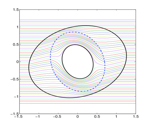
Figure 2: Ray paths through a non-radially symmetric cloak. The solid curves are the inner and outer surface of the cloak. The dashed curve delineates the inner region in which the deformation gradient is everywhere symmetric and the cloak is pure PM with finite isotropic mass. Two movies of the rays and wavefronts in this cloak may be viewed here.

5.2 Scattering from near-cloaks

A near-cloak or almost perfect cloak is defined here as one with inner surface $\partial\omega_{-}$ that does not correspond to the single point ${\mbox{\boldmath$\displaystyle\mathbf{X}$}}={\mbox{\boldmath$\displaystyle\mathbf{O}$}}$. We illustrate the issue using the radially symmetric deformation (16) with $f(a)$ small but non-zero, and assuming time harmonic motion, with the factor $e^{-ikt}$ understood but omitted. Since the inner surface is not the image of a point, it is necessary to prescribe a boundary condition on the interior surface, which we take as zero pressure on $r=a$. The specific nature of the boundary condition should be irrelevant as $f(a)$ shrinks to zero.

As before, the cloak occupies $\omega=\{{\mbox{\boldmath$\displaystyle\mathbf{x}$}}:\,a\leq r\leq b\}$, but now $f(a)>0$. The total response for plane wave incidence is $p({\mbox{\boldmath$\displaystyle\mathbf{x}$}})=p_{0}e^{ikR(r)\cos\theta}+p_{sc}({\mbox{\boldmath$\displaystyle\mathbf{x}$}})$, where $p_{0}$ is a constant and

$$p_{sc}=-p_{0}\sum\limits_{n=0}^{\infty}\begin{cases}i^{n}(2-\delta_{n0})J_{n}(kR(a))\frac{H^{(1)}_{n}(kR(r))}{H^{(1)}_{n}(kR(a))}\cos n\theta,\\ i^{n}(2n+1)j_{n}(kR(a))\frac{h^{(1)}_{n}(kR(r))}{h^{(1)}_{n}(kR(a))}P_{n}(\cos\theta),\end{cases}\quad R(r)=\begin{cases}f(r),&a\leq r<b,\\ r,&b\leq r<\infty,\end{cases}$$

in 2D and 3D, respectively. A near-cloak can be defined in many ways: for instance, a power law $f(r)=b\big{(}\frac{r-\delta}{b-\delta}\big{)}^{\alpha}$ with $0<\delta<a$ is considered in [22]. Here we assume a linear near-cloak mapping similar to the one examined by Kohn et al. [20],

$$f^{(\delta)}(r)=b\big{(}\frac{r-a}{b-a}\big{)}+\delta\big{(}\frac{b-r}{b-a}\big{)},$$ (64)

where $0<\delta<a$. Hence, $f^{(\delta)}(a)=\delta$ and the radius at which the mapping is zero, $r=a-\delta(b-a)/(b-\delta)$, defines the size of a smaller but perfect cloak.

Some representative results are shown in Figure 3(b), which illustrates clearly a disparity between cylindrical and spherical cloaking, even when the physical optics cross-sections are identical. Thus, for $f(a)=0.01a$ the 3D cross-section is negligible (Fig. 3(b).d) but for 2D the cross-section is two orders of magnitude larger (Fig. 3(b).c). Ruan et al. [23] found that the perfect cylindrical EM cloak is sensitive to perturbation. This sensitivity is evident from the present analysis through the dependence on the length $\delta$ which measures the departure from perfect cloaking $(\delta=0)$.

 

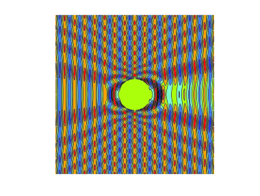
(a) 2D, $\delta=0.3$, $\Sigma=1.48$

(b) 3D, $\delta=0.3$, $\Sigma=0.79$

Figure 3: A plane wave is incident from the left with frequency $k=10$ on the cloak defined by eq. (64) with $a=1$, $b=2^{1/(d-1)}$. The outer cloak radius $b$ is chosen so that the geometrical cross-section of the cloak is twice the geometrical cross-section of the cloaked region in both 2D and 3D. The circular core in the plots is the cloaked region of radius $a$. The virtual inner radius $f(a)=\delta$ is $0.3$ or $0.01$, and $\Sigma$ is the total scattering cross-section.

 

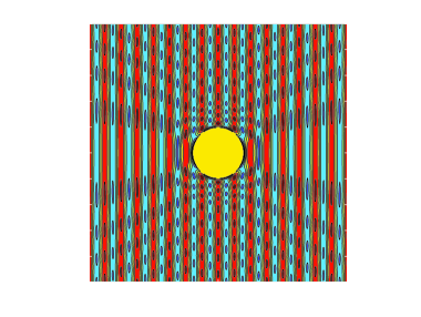
(c) 2D, $\delta=0.01$, $\Sigma=0.12$

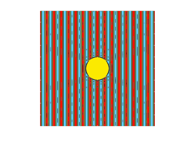
(d) 3D, $\delta=0.01$, $\Sigma=1\times 10^{-3}$

The ineffectiveness of the same cloak in 2D as compared with 3D can be understood in terms of the scattering cross-section. The leading order far-field is of the form $p=p_{0}e^{ikz}+p_{0}g(\hat{\mbox{\boldmath$\displaystyle\mathbf{x}$}})r^{-(d-1)/2}(i2\pi/k)^{(3-d)/2}e^{ikr}$. The optical theorem implies that the total scattering cross-section, and hence the total energy scattered, is determined by the forward scattering amplitude: $\Sigma=4\pi k^{-1}\text{Im}g(\hat{\mbox{\boldmath$\displaystyle\mathbf{e}$}}_{z})$. Thus,

$$\Sigma=\begin{cases}\frac{4}{k}\sum\limits_{n=0}^{\infty}(2-\delta_{n0})\text{Re}\frac{J_{n}(kf(a))}{H^{(1)}_{n}(kf(a))},&2D,\\ \frac{4\pi}{k^{2}}\sum\limits_{n=0}^{\infty}(2n+1)\text{Re}\frac{j_{n}(kf(a))}{h^{(1)}_{n}(kf(a))},&3D.\end{cases}$$ (65)

The cross-section is dominated in the small $kf(a)$ limit by the $n=0$ term, with leading order approximations

$$\Sigma=\begin{cases}\frac{\pi^{2}}{k}|\ln kf(a)|^{-2}+\ldots,&2D,\\ 4\pi f^{2}(a)+\ldots,&3D.\end{cases}$$ (66)

This explains the greater efficacy in 3D, and suggests that all things being equal, cylindrical cloaking is more difficult to achieve than its spherical counterpart.

6 Discussion and conclusion

Starting from the idea of an acoustic cloak defined by a finite deformation we have shown that the acoustic wave equation in the undeformed region is mapped into a variety of possible equations in the physical cloak. Theorem 1 implies that the general form of the wave equation in the cloak is

$$K{\mbox{\boldmath$\displaystyle\mathbf{S}$}}:\nabla\big{(}{\mbox{\boldmath$\displaystyle\mathbf{\rho}$}}^{-1}{\mbox{\boldmath$\displaystyle\mathbf{S}$}}\nabla p\big{)}-\ddot{p}=0,$$ (67)

where the stress-like symmetric tensor $\displaystyle\mathbf{S}$ is divergence free and the inertia tensor is ${\mbox{\boldmath$\displaystyle\mathbf{\rho}$}}=J{\mbox{\boldmath$\displaystyle\mathbf{S}$}}{\mbox{\boldmath$\displaystyle\mathbf{V}$}}^{-2}{\mbox{\boldmath$\displaystyle\mathbf{S}$}}$. The non-unique nature of $\displaystyle\mathbf{S}$ for a given fixed deformation opens many possibilities for interpreting the cloak in terms of material properties.

If $\displaystyle\mathbf{S}$ is constant (${\mbox{\boldmath$\displaystyle\mathbf{S}$}}={\mbox{\boldmath$\displaystyle\mathbf{I}$}}$ with no loss in generality) then the cloak material corresponds to an acoustic fluid with pressure $p$ defined by a single bulk modulus but with a mass density $\displaystyle\mathbf{\rho}$ that is anisotropic, which we call the inertial cloak (IC). The IC model is mathematically consistent but physically impossible because it requires a cloak of infinite total mass. There appears to be no way to avoid this if one restricts the cloak material properties to the IC model. If one is willing to use an imperfect cloak with finite mass, and is concerned with fixed frequency waves, then the scattering examples show that significant cloaking can be obtained by shrinking the effective visible radius to be subwavelength. The 2D and 3D responses for imperfect cloaking are quite distinct, with far better results found in 3D.

A cloak of finite mass is achievable by allowing $\displaystyle\mathbf{S}$ to be spatially varying and divergence free. The general material associated with eq. (67), called PM-IC, has both anisotropic inertia and anisotropic elastic properties. The elastic stiffness tensor has the form of a pentamode material (PM) characterized by the symmetric tensor $\displaystyle\mathbf{S}$ and a single modulus $K$. Under certain circumstances, characterized in Lemmas 4 and 5, the density becomes isotropic and the material is pure PM. More importantly, the total mass can be made finite.

The finite mass problem arises from how we interpret the cloak material in the neighbourhood of its inner surface. It is therefore not necessary to totally abandon the pure IC model, but it does mean that the alternative PM-IC is required at the inner surface. From the examples considered here it appears that one can always use a pure PM model near the inner cloak surface, and thereby achieve finite mass. One method is to force the deformation near the inner surface to be a pure stretch, then Lemma 5 implies that the density is locally $\rho=1/\det{\mbox{\boldmath$\displaystyle\mathbf{F}$}}$. The total mass remains finite as long as $\rho$ is locally integrable, which is easily achieved.

The theory and simulations of PM-IC and PM materials presented here illustrate the wealth of possible material properties that are opened up through the general PM-IC model of acoustic cloaking. Physical implementation is in principle feasible: for instance, anisotropic inertia can be achieved by microlayers of inviscid acoustic fluid [11], while the microstructure required for pentamode materials has been described [18]. It remains to combine these known methods to obtain practical PM-IC materials.

Acknowledgments

Constructive suggestions from the anonymous reviewers are appreciated.

Appendix

A Proof of Theorem 1

A weak but instructive form of the identity (41) is proved first. Consider the possible identity

$$\nabla_{X}^{2}p=c{\mbox{\boldmath$\displaystyle\mathbf{A}$}}:\nabla\big{(}{\mbox{\boldmath$\displaystyle\mathbf{B}$}}^{-2}\operatorname{div}c^{-1}{\mbox{\boldmath$\displaystyle\mathbf{A}$}}p\big{)},$$ (A.1)

where $\displaystyle\mathbf{A}$, ${\mbox{\boldmath$\displaystyle\mathbf{B}$}}\in$Sym are non-singular and $c$ is a scalar. Let us examine under what circumstances this identity holds. Let $q$ be an arbitrary test function, and consider the integral

$$I=\int_{\Omega}\operatorname{d}V\,q\,c{\mbox{\boldmath$\displaystyle\mathbf{A}$}}:\nabla\big{(}{\mbox{\boldmath$\displaystyle\mathbf{B}$}}^{-2}\operatorname{div}c^{-1}{\mbox{\boldmath$\displaystyle\mathbf{A}$}}p\big{)}.$$ (A.2)

Substituting $\operatorname{d}V=J^{-1}\operatorname{d}v$, integrating by parts and ignoring surface contributions, yields

$$I=-\int_{\omega}\operatorname{d}v\,\big{(}\operatorname{div}J^{-1}c{\mbox{\boldmath$\displaystyle\mathbf{A}$}}q\big{)}\cdot\big{(}{\mbox{\boldmath$\displaystyle\mathbf{B}$}}^{-2}\operatorname{div}c^{-1}{\mbox{\boldmath$\displaystyle\mathbf{A}$}}p\big{)}.$$ (A.3)

In order to guarantee the integral is self-adjoint, that is, symmetric in both $p$ and $q$, we demand $c=J^{1/2}$. The self-adjoint property is made evident by writing $I$ as

$$I=-\int_{\omega}\operatorname{d}v\,\big{(}{\mbox{\boldmath$\displaystyle\mathbf{B}$}}^{-1}\operatorname{div}J^{-1/2}{\mbox{\boldmath$\displaystyle\mathbf{A}$}}q\big{)}\cdot\big{(}{\mbox{\boldmath$\displaystyle\mathbf{B}$}}^{-1}\operatorname{div}J^{-1/2}{\mbox{\boldmath$\displaystyle\mathbf{A}$}}p\big{)}.$$ (A.4)

If (A.1) is to be valid, then

$$I=-\int_{\Omega}\operatorname{d}V\,\nabla_{X}q\cdot\nabla_{X}p.$$ (A.5)

Comparing these integrals and once again using $\operatorname{d}v=J\operatorname{d}V$, implies

$$\big{(}J^{1/2}{\mbox{\boldmath$\displaystyle\mathbf{B}$}}^{-1}\operatorname{div}J^{-1/2}{\mbox{\boldmath$\displaystyle\mathbf{A}$}}q\big{)}\cdot\big{(}J^{1/2}{\mbox{\boldmath$\displaystyle\mathbf{B}$}}^{-1}\operatorname{div}J^{-1/2}{\mbox{\boldmath$\displaystyle\mathbf{A}$}}p\big{)}=\nabla_{X}q\cdot\nabla_{X}p.$$ (A.6)

The only way that these can agree for arbitrary $p$ and $q$ is if

$$\operatorname{div}J^{-1/2}{\mbox{\boldmath$\displaystyle\mathbf{A}$}}=0,$$ (A.7)

in which case (A.6) becomes

$$\big{(}{\mbox{\boldmath$\displaystyle\mathbf{B}$}}^{-1}{\mbox{\boldmath$\displaystyle\mathbf{A}$}}{\mbox{\boldmath$\displaystyle\mathbf{F}$}}^{-t}\nabla_{X}q\big{)}\cdot\big{(}{\mbox{\boldmath$\displaystyle\mathbf{B}$}}^{-1}{\mbox{\boldmath$\displaystyle\mathbf{A}$}}{\mbox{\boldmath$\displaystyle\mathbf{F}$}}^{-t}\nabla_{X}p\big{)}=\nabla_{X}q\cdot\nabla_{X}p.$$ (A.8)

Using ${\mbox{\boldmath$\displaystyle\mathbf{V}$}}^{2}={\mbox{\boldmath$\displaystyle\mathbf{F}$}}{\mbox{\boldmath$\displaystyle\mathbf{F}$}}^{t}$, it is clear that (A.8) can only be satisfied if

$${\mbox{\boldmath$\displaystyle\mathbf{B}$}}^{-2}={\mbox{\boldmath$\displaystyle\mathbf{A}$}}^{-1}{\mbox{\boldmath$\displaystyle\mathbf{V}$}}^{2}{\mbox{\boldmath$\displaystyle\mathbf{A}$}}^{-1}.$$ (A.9)

A weak form of Theorem 1 follows by substituting ${\mbox{\boldmath$\displaystyle\mathbf{A}$}}=J^{1/2}{\mbox{\boldmath$\displaystyle\mathbf{P}$}}$. Based upon this it is a straightforward exercise to see that the identity (41) can be derived directly by brute force differentiation of the right hand side, taking into account the constraint (42) and Lemma 1.

B Ray equations in an acoustic cloak

Consider a WKB type of solution for the displacement: ${\mbox{\boldmath$\displaystyle\mathbf{u}$}}({\mbox{\boldmath$\displaystyle\mathbf{x}$}},t)={\mbox{\boldmath$\displaystyle\mathbf{U}$}}({\mbox{\boldmath$\displaystyle\mathbf{x}$}},t)e^{ik\phi({\mbox{\boldmath$\displaystyle\mathbf{x}$}},t)}$. The leading order equation for the phase $\phi$ and amplitude $\displaystyle\mathbf{U}$ is (see eqs. (33)-(38))

$$\big{[}K\,({\mbox{\boldmath$\displaystyle\mathbf{S}$}}{\nabla\phi})\otimes({\mbox{\boldmath$\displaystyle\mathbf{S}$}}{\nabla\phi})-\dot{\phi}^{2}{\mbox{\boldmath$\displaystyle\mathbf{\rho}$}}\big{]}{\mbox{\boldmath$\displaystyle\mathbf{U}$}}=0.$$ (B.1)

The inner product of eq. (B.1) with $\displaystyle\mathbf{U}$ may be written $H_{+}H_{-}=0$ where

$$H_{\pm}=\dot{\phi}\pm K^{1/2}|\hat{\mbox{\boldmath$\displaystyle\mathbf{q}$}}\cdot{\mbox{\boldmath$\displaystyle\mathbf{\rho}$}}^{-1/2}{\mbox{\boldmath$\displaystyle\mathbf{S}$}}{\nabla\phi}|,$$ (B.2)

and $\hat{\mbox{\boldmath$\displaystyle\mathbf{q}$}}={\mbox{\boldmath$\displaystyle\mathbf{\rho}$}}^{1/2}{\mbox{\boldmath$\displaystyle\mathbf{U}$}}/|{\mbox{\boldmath$\displaystyle\mathbf{\rho}$}}^{1/2}{\mbox{\boldmath$\displaystyle\mathbf{U}$}}|$. We focus on the characteristic $H_{+}(\dot{\phi},\nabla\phi,{\mbox{\boldmath$\displaystyle\mathbf{x}$}})=0$. The Hamilton-Jacobi equations for this “Hamiltonian” yield the ray equations,

$$\frac{\operatorname{d}t}{\operatorname{d}\tau}=\frac{\partial H_{+}}{\partial\dot{\phi}},\qquad\frac{\operatorname{d}{\mbox{\boldmath$\displaystyle\mathbf{x}$}}}{\operatorname{d}\tau}=\frac{\partial H_{+}}{\partial\nabla\phi},\qquad\frac{\operatorname{d}\nabla\phi}{\operatorname{d}\tau}=-\frac{\partial H_{+}}{\partial{\mbox{\boldmath$\displaystyle\mathbf{x}$}}},\qquad\frac{\operatorname{d}\dot{\phi}}{\operatorname{d}\tau}=-\frac{\partial H_{+}}{\partial t},$$ (B.3)

where $\tau$ is the time-like ray parameter. Since ${\partial H_{+}}/{\partial\dot{\phi}}=1$, $\tau$ may be replaced by $t$ as the natural ray parameter, while ${\partial H_{+}}/{\partial t}=0$ implies that $\dot{\phi}$ is constant along a ray. We choose $\dot{\phi}=-1$ for convenience. Define the slowness vector ${\mbox{\boldmath$\displaystyle\mathbf{s}$}}(\tau)=\nabla\phi$ along the ray ${\mbox{\boldmath$\displaystyle\mathbf{x}$}}={\mbox{\boldmath$\displaystyle\mathbf{x}$}}(\tau)$. The vector equation (B.1) then implies that $\hat{\mbox{\boldmath$\displaystyle\mathbf{q}$}}=K^{1/2}{\mbox{\boldmath$\displaystyle\mathbf{\rho}$}}^{-1/2}{\mbox{\boldmath$\displaystyle\mathbf{S}$}}{\mbox{\boldmath$\displaystyle\mathbf{s}$}}$, and since $\hat{\mbox{\boldmath$\displaystyle\mathbf{q}$}}$ is by definition a unit vector, using eq. (43b) we deduce that the slowness satisfies

$${\mbox{\boldmath$\displaystyle\mathbf{s}$}}\cdot{\mbox{\boldmath$\displaystyle\mathbf{V}$}}^{2}{\mbox{\boldmath$\displaystyle\mathbf{s}$}}=1.$$ (B.4)

This is simply the ellipsoidal slowness surface mentioned in Section 4. Finally, the evolution equations along the ray can be expressed as a closed system for ${\mbox{\boldmath$\displaystyle\mathbf{x}$}}(t),{\mbox{\boldmath$\displaystyle\mathbf{s}$}}(t)$ by using eq. (B.3) and noting that $H_{+}=\big{(}{\mbox{\boldmath$\displaystyle\mathbf{s}$}}\cdot{\mbox{\boldmath$\displaystyle\mathbf{V}$}}^{2}{\mbox{\boldmath$\displaystyle\mathbf{s}$}}\big{)}^{1/2}-1$,

$$\frac{\operatorname{d}{\mbox{\boldmath$\displaystyle\mathbf{x}$}}}{\operatorname{d}t}={\mbox{\boldmath$\displaystyle\mathbf{V}$}}^{2}{\mbox{\boldmath$\displaystyle\mathbf{s}$}},\qquad\frac{\operatorname{d}{\mbox{\boldmath$\displaystyle\mathbf{s}$}}}{\operatorname{d}t}=-({\mbox{\boldmath$\displaystyle\mathbf{V}$}}{\mbox{\boldmath$\displaystyle\mathbf{s}$}})\cdot(\nabla{\mbox{\boldmath$\displaystyle\mathbf{V}$}}){\mbox{\boldmath$\displaystyle\mathbf{s}$}}.$$ (B.5)

References

• [1] A. J. Ward and J. B. Pendry. Refraction and geometry in Maxwell’s equations. J. Modern Optics, 43(4):773–793, 1996.
• [2] E. J. Post. Formal Structure of Electromagnetics: General Covariance and Electromagnetics. Interscience, New York, 1962.
• [3] A. Greenleaf, M. Lassas, and G. Uhlmann. On nonuniqueness for Calderon’s inverse problem. Math. Res. Lett., 10:685–693, Jul 2003.
• [4] A. Greenleaf, M. Lassas, and G. Uhlmann. Anisotropic conductivities that cannot be detected by EIT. Physiol. Meas., 24(2):413–419, May 2003.
• [5] J. B. Pendry, D. Schurig, and D. R. Smith. Controlling electromagnetic fields. Science, 312(5781):1780–1782, June 2006.
• [6] U. Leonhardt. Optical conformal mapping. Science, 312(5781):1777–1780, June 2006.
• [7] S. A. Cummer and D. Schurig. One path to acoustic cloaking. New J. Phys., 9(3):45+, March 2007.
• [8] H. Chen and C. T. Chan. Acoustic cloaking in three dimensions using acoustic metamaterials. Appl. Phys. Lett., 91(18):183518+, 2007.
• [9] S. A. Cummer, B. I. Popa, D. Schurig, D. R. Smith, J. Pendry, M. Rahm, and A. Starr. Scattering theory derivation of a 3D acoustic cloaking shell. Phys. Rev. Lett., 100(2):024301+, 2008.
• [10] G. W. Milton, M. Briane, and J. R. Willis. On cloaking for elasticity and physical equations with a transformation invariant form. New J. Phys., 8:248–267, 2006.
• [11] M. Schoenberg and P. N. Sen. Properties of a periodically stratified acoustic half-space and its relation to a Biot fluid. J. Acoust. Soc. Am., 73(1):61–67, 1983.
• [12] J. Mei, Z. Liu, W. Wen, and P. Sheng. Effective dynamic mass density of composites. Phys. Rev. B, 76(13):134205+, 2007.
• [13] D. Torrent and J. Sánchez-Dehesa. Anisotropic mass density by two-dimensional acoustic metamaterials. New J. Phys., 10(2):023004+, 2008.
• [14] G. W. Milton and J. R. Willis. On modifications of Newton’s second law and linear continuum elastodynamics. Proc. R. Soc. A, 463(2079):855–880, March 2007.
• [15] D. Schurig, J. J. Mock, B. J. Justice, S. A. Cummer, J. B. Pendry, A. F. Starr, and D. R. Smith. Metamaterial electromagnetic cloak at microwave frequencies. Science, 314(5801):977–980, November 2006.
• [16] A. Greenleaf, Y. Kurylev, M. Lassas, and G. Uhlmann. Full-wave invisibility of active devices at all frequencies. Comm. Math. Phys., 275(3):749–789, November 2007.
• [17] A. Greenleaf, Y. Kurylev, M. Lassas, and G. Uhlmann. Comment on ”Scattering theory derivation of a 3D acoustic cloaking shell”. Jan 2008. URL
• [18] G. W. Milton and A. V. Cherkaev. Which elasticity tensors are realizable? J. Eng. Mater. Tech., 117(4):483–493, 1995.
• [19] R. W. Ogden. Non-Linear Elastic Deformations. Dover Publications, 1997.
• [20] R. V. Kohn, H. Shen, M. S. Vogelius, and M. I. Weinstein. Cloaking via change of variables in electric impedance tomography. Inverse Problems, 24(1):015016+, 2008.
• [21] M. J. P. Musgrave. Crystal Acoustics. Acoustical Society of America, New York, 2003.
• [22] A. N. Norris. Acoustic cloaking in 2D and 3D using finite mass, Feb 2008. URL
• [23] Z. Ruan, M. Yan, C. W. Neff, and M. Qiu. Ideal cylindrical cloak: Perfect but sensitive to tiny perturbations. Phys. Rev. Lett., 99(11):113903 +, 2007.