Final Results from the KTeV Experiment on the Decay $K_{L}\to\pi^{0}\gamma\gamma$

Abstract

We report on a new measurement of the branching ratio B($K_{L}\to\pi^{0}\gamma\gamma$) using the KTeV detector. We reconstruct 1982 events with an estimated background of 608, that results in B($K_{L}\to\pi^{0}\gamma\gamma$) = $(1.29\pm 0.03_{stat}\pm 0.05_{syst})\times 10^{-6}$. We also measure the parameter, $a_{V}$, which characterizes the strength of vector meson exchange terms in this decay. We find $a_{V}=-0.31\pm 0.05_{stat}\pm 0.07_{syst}$. These results utilize the full KTeV data set collected from 1997 to 2000 and supersede earlier KTeV measurements of the branching ratio and $a_{V}$.

I Introduction

The decay $K_{L}\to\pi^{0}\gamma\gamma$ provides important checks of low-energy theories of strange meson decays. In Chiral Perturbation Theory (ChPT) the branching ratio for this decay can be determined with no free parameters up to $O(p^{4})$. However, the first measurements of the branching ratio for $K_{L}\to\pi^{0}\gamma\gamma$ ref:na31a ; ref:e731 ; ref:na31b were approximately three times larger than the predicted $O(p^{4})$ branching ratio of $0.68\times 10^{-6}$ref:ecker . Extending the theory to $O(p^{6})$ and including vector meson exchange terms raise the branching ratio prediction to be consistent with the measured valuesref:dambrosio ; ref:gabbiani . The vector meson contributions can be parametrized by an effective coupling constant $a_{V}$. Non perturbative calculations for the $K_{L}\to\pi^{0}\gamma\gamma$ rate have also been performedref:truong .

The $K_{L}\to\pi^{0}\gamma\gamma$ decay is important also because of its implications for the related decay $K_{L}\to\pi^{0}l^{+}l^{-}$, where $l^{+}l^{-}$ can be either $e^{+}e^{-}$ or $\mu^{+}\mu^{-}$. Currently, the best limits for these decays are B($K_{L}\to\pi^{0}e^{+}e^{-}$) $<2.8\times 10^{-10}$ref:pi0ee and B($K_{L}\to\pi^{0}\mu^{+}\mu^{-}$) $<3.8\times 10^{-10}$ref:pi0mm , both at the 90% confidence level. The expected branching ratios are approximately $1-43\times 10^{-11}$ref:buchalla ; ref:mescia . There are three contributions to the $K_{L}\to\pi^{0}l^{+}l^{-}$ decay, classified in terms of their CP symmetry; one conserves CP symmetry, one violates it indirectly and one directly. The direct CP violating amplitude is of interest within the Standard Model but also can show signs of new physics ref:mescia , leading to an enhancement of the $K_{L}\to l^{+}l^{-}$ rate. In order to determine the direct CP violating terms, one must first determine the other two amplitudes. The indirect CP violating amplitude can be determined from the decay $K_{S}\to\pi^{0}l^{+}l^{-}$, and the NA48 experiment has measured B($K_{S}\to\pi^{0}e^{+}e^{-}$) $=5.8^{+2.9}_{-2.4}\times 10^{-9}$.ref:ksp0ee . Because the $K_{L}\to\pi^{0}l^{+}l^{-}$ decay can proceed via a CP conserving two-photon exchange, the CP conserving terms can be probed using $K_{L}\to\pi^{0}\gamma\gamma$. A precise measurement of the parameter $a_{V}$ can be used to determine the size of the CP conserving amplitude in $K_{L}\to\pi^{0}l^{+}l^{-}$.

There have been a number of previous measurements of $K_{L}\to\pi^{0}\gamma\gamma$ from the E731, NA31, NA48 and KTeV experiments.ref:na31a ; ref:e731 ; ref:na31b ; ref:ktev ; ref:NA48 . The two most recent measurements are the NA48 result of $(1.36\pm 0.03_{stat}\pm 0.03_{syst}\pm 0.03_{norm})\times 10^{-6}$ and the KTeV result of $(1.68\pm 0.07_{stat}\pm 0.08_{syst})\times 10^{-6}$. Both of these results are significantly more precise than the E731 and NA31 results. However, the NA48 and KTeV results differ by nearly three standard deviations. The measurement discussed here supersedes the previous KTeV result and reconciles the difference between these two results.

II The KTeV Detector

Data used in this analysis were collected during three running periods in 1996, 1997 and 1999 using the KTeV detector at Fermilab. Because of the similar topology between the $K_{L}\to\pi^{0}\gamma\gamma$ decays and the $K_{L}\to\pi^{0}\pi^{0}$ decays used to measure $\epsilon^{\prime}/\epsilon$ ref:epp97 , we recorded the $K_{L}\to\pi^{0}\gamma\gamma$ events during the same collection period used for the KTeV $\epsilon^{\prime}/\epsilon$ measurement.

The KTeV experimentref:detector is a fixed-target experiment built to study decays of neutral kaons. A schematic of the detector is shown in Figure 1. Two neutral kaon beams were produced through interactions of 800 GeV/$c$ protons in a 30 cm long beryllium oxide target. The resulting neutral particles passed through a series of collimators and absorbers to produce two nearly parallel beams. Charged particles were removed from the beams by sweeping magnets located downstream of the collimators. A vacuum decay volume extended from 94 to 159 meters downstream of the target, and was far enough away from the target that the vast majority of the $K_{S}$ component had decayed away. An active regenerator was located within the vacuum region, approximately 123 meters downstream of the target. This regenerator alternated between the two neutral beams to generate a $K_{S}$ component in one of the beams. The beam that coincided with the regenerator was called the regenerator beam, while the other beam was denoted the vacuum beam. For this analysis, we only considered decays from the vacuum beam. To reject photons, primarily from decays of $K_{L}\to\pi^{0}\pi^{0}\pi^{0}$, the decay volume was surrounded by photon veto detectors, that rejected photons produced at angles greater than 100 milliradians with laboratory energies greater than 100 MeV. A kevlar and mylar vacuum window with a radiation length of 0.14% covered the downstream end of the vacuum decay region.

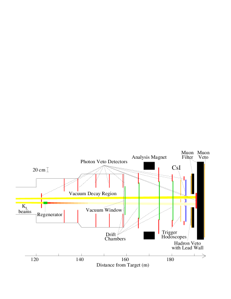
Figure 1: Schematic of the KTeV detector.

The most critical detector element in this analysis was the pure CsI electromagnetic calorimeterref:epp97 . The CsI calorimeter, shown in Figure 2, was composed of 3100 blocks in a 1.9 m by 1.9 m array with a depth of 50 cm corresponding to 27 radiation lengths. Two 15 cm by 15 cm holes were located near the center of the array for the passage of the neutral beams. For photons with energies between 2 and 60 GeV, the calorimeter energy resolution was below 1% and the nonlinearity was less than 0.5% per 100 GeV. The position resolution of the calorimeter was approximately 1 mm.

Figure 2: Transverse view of the KTeV CsI calorimeter. The smaller blocks are located in the central region with the larger blocks located in the outer region.

Two levels of hardware triggers were used in the KTeV experiment. For the $K_{L}\to\pi^{0}\gamma\gamma$ events, the first level trigger required the event to deposit more than approximately 25 GeV in the CsI calorimeter with less than 100 MeV in any of the photon vetoes. The second level trigger utilized a hardware cluster processor that counted the number of separate clusters in the CsI calorimeterhcc . Each cluster had to have an energy greater than approximately 1.0 GeV and the total number of clusters in the CsI calorimeter was required to be equal to four.

Events that satisfied the hardware triggers were also required to satisfy an online software filter. This filter required that one of the six possible combinations of two photons reconstructed near the $\pi^{0}$ mass. In addition, the filter required that the decay vertex reconstructed upstream of 155 m for the 1996-1997 data and 140 m for the 1999 data. This requirement was tightened for the 1999 data to help reduce the trigger rate for the $K_{L}\to\pi^{0}\gamma\gamma$ sample. These trigger requirements also selected $K_{L}\to\pi^{0}\pi^{0}$ events which were used as a normalization mode for calculating the $K_{L}\to\pi^{0}\gamma\gamma$ branching ratio.

III Event Reconstruction

The $K_{L}\to\pi^{0}\gamma\gamma$ final state consists of four photons with no other activity in the detector. In this analysis we require that all events have exactly four clusters in the CsI calorimeter and that the energy of each cluster is greater than 2.0 GeV. To reduce contamination from events originating from the regenerator beam, the center of energy (Eq. 9 of ref:epp97 ) is required to be within the CsI beam hole corresponding to the vacuum beam.

In the decay $K_{L}\to\pi^{0}\gamma\gamma$ the positions and energies of the four photons do not provide enough constraints to determine both the decay position and the invariant mass of the system. Therefore, we assume that the four-photon invariant mass is equal to the kaon mass, and reconstruct the decay vertex position ($z$) from the calorimeter information. For a $\pi^{0}$ decaying into two photons, one can determine the two-photon mass using the following relation:

$$m_{12}\approx\frac{\sqrt{E_{1}E_{2}}r_{12}}{\Delta z_{CsI}}$$ (1)

where $E_{1}$ and $E_{2}$ are the energies of the two photons, $r_{12}$ is the distance between the two photons at the CsI calorimeter, and $\Delta z_{CsI}$ is the distance between the decay vertex and the CsI calorimeter. Using the position of the reconstructed decay vertex, we determine the two-photon mass for each of the six possible combinations and choose the combination with the reconstructed mass closest to the known $\pi^{0}$ mass. If the closest mass combination differs by more than 3 MeV/$c^{2}$ from the known $\pi^{0}$ mass, we reject the event. The total energy of the kaon system, determined from summing the energies of the four clusters, is required to be between 40 and 160 GeV. After these requirements the data sample is dominated by backgrounds from $K_{L}\to\pi^{0}\pi^{0}\pi^{0}$ and $K_{L}\to\pi^{0}\pi^{0}$ decays. Additional cuts described in Section V are used to reduce these backgrounds.

IV Monte Carlo Simulation

A detailed Monte Carlo simulation was used to estimate the detector acceptance and the background level in our final sample. Our Monte Carlo simulates the kaon production at the target and propagates the kaon amplitude through the detector. The kaon then decays according to the appropriate decay mode, and the resulting daughter particles are traced through the KTeV detector. The interaction of the decay products with the detector is simulated and the detector response is then digitized.

Details of the simulation for all detector components are given in ref:epp97 ; here we focus on the simulation of the CsI calorimeter. To simulate the response of the CsI calorimeter, we used a library of photons generated using GEANT simulationsref:GEANT . The library contained information deposited into a $13\times 13$ array of CsI crystals. The wrapping and shims separating each crystal was included in these simulations. This library was binned as a function of the energy and position of the incident photon. We stored the energy depositions for each crystal in 10 longitudinal bins to include the effects of nonlinear response along the length of the crystal.

During the course of our studies we found that the GEANT-based shower library was not adequate for describing the transverse distribution of the energy in a electromagnetic shower. As noted below, we make use of this transverse shape to help reduce backgrounds from $K_{L}\to\pi^{0}\pi^{0}\pi^{0}$ decays. To better simulate the shower shapes, we also implemented a data-based shower library. These showers were extracted from $K_{L}\to\pi^{0}\pi^{0}$ events taken during special, low-intensity runs to reduce the effects of accidental activity in the CsI calorimeter. The data-based shower library was also binned as a function of the incident photon energy and the incident position.

To characterize the transverse energy deposition of a electromagnetic shower, we devised a photon shape $\chi^{2}$ variable. This variable compares the energy in the central $3\times 3$ crystals of a cluster to the expected energy distribution. While a $7\times 7$ array of crystals is used for accurate cluster energy reconstruction, the photon shape $\chi^{2}$ is determined from the central $3\times 3$ crystals to minimize any biases from accidental activity. As shown in Figure 3, Monte Carlo events utilizing the data-based shower library match the data better compared to the GEANT-based shower library. For our Monte Carlo samples, we utilized both shower libraries. The GEANT-based shower library was used to determine the energy and position of the cluster, while the data-based shower library was used for extracting the transverse shape information.

Figure 3: The photon shape $\chi^{2}$ variable. a) The photon shape $\chi^{2}$ variable for $K_{L}\to\pi^{0}\pi^{0}$ with the dots representing the data and the solid histogram the Monte Carlo simulation. The Monte Carlo simulation was generated using our GEANT-based shower library. b) The photon shape $\chi^{2}$ variable for $K_{L}\to\pi^{0}\pi^{0}$ events. The dots are the data and the histogram represents the Monte Carlo simulation using our data-based shower library. The data-based Monte Carlo simulation shows marked improvement over the GEANT-based shower library.

V Backgrounds to $K_{L}\to\pi^{0}\gamma\gamma$

After the event reconstruction discussed in Section III, large backgrounds remain in our data sample. Here we discuss the additional criteria used to reduce these backgrounds. The major backgrounds in our data sample consist of events with neutral beam particles interacting in the vacuum window, kaon decays with charged tracks, $K_{L}\to\pi^{0}\pi^{0}$ decays, and $K_{L}\to\pi^{0}\pi^{0}\pi^{0}$ decays, with the $K_{L}\to\pi^{0}\pi^{0}\pi^{0}$ decays being the most difficult to remove. Vacuum window interactions can produce $\pi^{0}\pi^{0}$ and $\pi^{0}\eta$ pairs. To remove the vacuum window interactions, we loop over the six possible two photon combinations and determine the two-photon decay vertex assuming the photons resulted from a $\pi^{0}$ decay. For each of the six possible combinations, we reject the event if the decay vertex is downstream of the vacuum window and the invariant mass of the other $\gamma\gamma$ combination is near the neutral pion or $\eta$ mass. Events with charged tracks are removed by requiring that the total number of hits in the drift chamber system is less than 24; a two-track event will produce 32 hits in the drift chambers.

The $K_{L}\to\pi^{0}\pi^{0}$ events are easily identifiable because both $\gamma\gamma$ pairs will reconstruct with $m_{\gamma\gamma}\sim m_{\pi^{0}}$ mass. Almost all of these events are removed by rejecting events in which both $\gamma\gamma$ masses ($m_{12}$ and $m_{34}$) are near the $\pi^{0}$ mass. $m_{12}$ is the two-photon invariant mass closest to the $\pi^{0}$ mass, while $m_{34}$ is the invariant mass of the other pair of photons. In about two percent of the $K_{L}\to\pi^{0}\pi^{0}$ events, our choice for $m_{12}$ and $m_{34}$ did not correctly choose both $\pi^{0}\to\gamma\gamma$ decays, and so the cut to remove the $K_{L}\to\pi^{0}\pi^{0}$ background fails. To remove these events, we also examine the other two possible combinations of the four photons and discard any event in which both the $m_{12}$ and $m_{34}$ values are near the mass of the $\pi^{0}$.

Because we required exactly four photons, $K_{L}\to\pi^{0}\pi^{0}\pi^{0}$ decays can only contribute to the background if some of the photons miss the calorimeter or two or more photons “fuse” together in the calorimeter. To reduce backgrounds from decays with missing photons, we remove events with any significant energy in any of the photon vetoes. Also, by restricting the decay region to $115<z<128$, we reduce the $K_{L}\to\pi^{0}\pi^{0}\pi^{0}$ background significantly because events with missing photons tend to have a reconstructed decay vertex downstream of the true decay position. As shown in Figure 4, the decay vertex distribution for $K_{L}\to\pi^{0}\pi^{0}$ events is relatively flat downstream of 120 meters. However, the $K_{L}\to\pi^{0}\pi^{0}\pi^{0}$ background rises sharply as the decay vertex position increases.

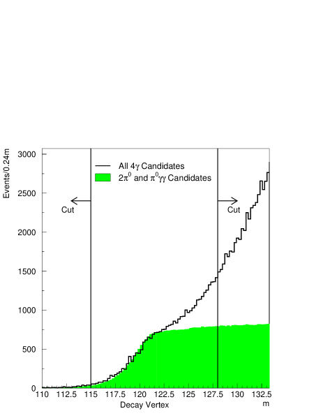
Figure 4: The reconstructed decay vertex position from four photons for all events (histogram) prior to imposing the decay vertex cut. All cuts except for the decay vertex and photon shape $\chi^{2}$ have been applied. The shaded histogram indicates $K_{L}\to\pi^{0}\pi^{0}$ and $K_{L}\to\pi^{0}\gamma\gamma$ candidates. The rise at large values is due to $K_{L}\to\pi^{0}\pi^{0}\pi^{0}$ decays in which one or more photons misses the CsI calorimeter. The position of the cut is indicated by the two vertical lines.

After applying the cuts described above, there still remains a significant number of $K_{L}\to\pi^{0}\pi^{0}\pi^{0}$ decays; far more than the signal from $K_{L}\to\pi^{0}\gamma\gamma$. These decays result primarily from events in which two of the CsI clusters come from fused photons. To remove these events, we select events with a small photon shape $\chi^{2}$. For non-fused clusters this variable peaks near zero, while for fused clusters this shape $\chi^{2}$ variable becomes quite large. Figure 5 shows this variable for both the data and for the $K_{L}\to\pi^{0}\pi^{0}\pi^{0}$ background. We require the shape $\chi^{2}$ to be less than 1.8. This cut was chosen to maximize the signal significance. For $K_{L}\to\pi^{0}\pi^{0}\pi^{0}$ background events we verified the photon shape $\chi^{2}$ distribution in the signal region by reweighting events from the tails of the $\pi^{0}$ mass distribution and found the resulting shape to correspond to our Monte Carlo prediction. The photon shape $\chi^{2}$ is our final cut, and reduces our background to a reasonable level.

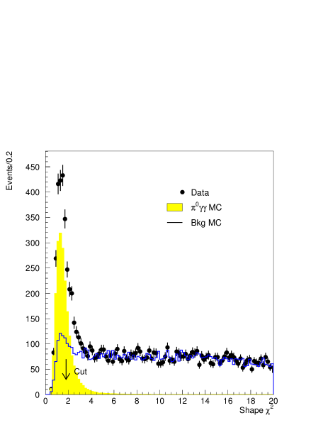
Figure 5: The photon shape $\chi^{2}$ variable. The solid histogram shows the $K_{L}\to\pi^{0}\pi^{0}\pi^{0}$ Monte Carlo while the dotted histogram is the data. The $K_{L}\to\pi^{0}\gamma\gamma$ signal Monte Carlo simulation is the shaded histogram. The sum of the signal plus background Monte Carlo simulation agrees well with the data.

VI Branching Ratio and $a_{V}$ Determination

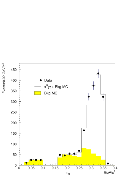
Figure 6: The $m_{34}$ mass distribution for after all selection cuts. The dots show the data, the histogram the sum of the signal and background Monte Carlo samples, and the shaded histogram the scaled background Monte Claro simulation.

After applying all of the cuts described above we find 1982 events before subtracting background. The final $m_{34}$ mass distribution is shown in Figure 6, with the data well-represented by the signal plus background Monte Carlo simulation. The background comprises approximately 30% of the total event sample.

To determine the $K_{L}\to\pi^{0}\gamma\gamma$ branching fraction, we use the following expression

$$B = ((N_{tot}-N_{bkg})/N_{2\pi^{0}})\times(\epsilon_{2\pi^{0}}/\epsilon_{\pi^{0}\gamma\gamma})$$ (2)

$$\times B(K_{L}\to\pi^{0}\pi^{0})\times B(\pi^{0}\to\gamma\gamma),$$

where $N_{tot}$ is the number of candidate events, $N_{bkg}$ is the number of background events, $N_{2\pi^{0}}$ is the number of normalization events, and $\epsilon_{2\pi^{0}}$ and $\epsilon_{\pi^{0}\gamma\gamma}$ are the acceptances of the $K_{L}\to\pi^{0}\pi^{0}$ and $K_{L}\to\pi^{0}\gamma\gamma$ events, respectively. The acceptances were determined using our Monte Carlo simulation described above. The value $B(K_{L}\to\pi^{0}\pi^{0})$ is the measured $K_{L}\to\pi^{0}\pi^{0}$ branching ratio. In the previous KTeV analysis, the value of B($K_{L}\to\pi^{0}\pi^{0}$) used was $(9.36\pm 0.2)\times 10^{-4}$. We are now using the most recent determination of B($K_{L}\to\pi^{0}\pi^{0}$) = $(8.69\pm 0.08)\times 10^{-4}$ref:2pi0BR ; ref:PDG . To determine the number of $K_{L}\to\pi^{0}\pi^{0}$ normalization decays, we count the number of events in the region, $0.130\ \mbox{GeV/$c^{2}$}<m_{34}<0.140\ \mbox{GeV/$c^{2}$}$. The kaon energy and decay vertex for our normalization mode are shown in Figure 7. There is good agreement between the data and Monte Carlo simulation.

Figure 7: The a) energy and b) decay vertex for $K_{L}\to\pi^{0}\pi^{0}$ decays. The dots are the data and the histogram is the Monte Carlo simulation.

The numbers used for the branching ratio determination are shown in Table 1. Note that the acceptances for the signal and normalization modes are nearly identical; this helps to significantly reduce the systematic uncertainties due to the acceptance calculation.

Parameter	1996-1997	1999	Total
$N_{tot}$	989	993	1982
$N_{tot}-N_{bkg}$	670.6	703.8	1374.4
$N_{2\pi^{0}}$ Events	482027	437305	919332
Signal Acceptance	0.0330	0.0261	0.030
Norm Acceptance	0.0328	0.0257	0.030
$K_{L}\to 3\pi^{0}$ Bkg	313	288	601
$K_{L}\to 2\pi^{0}$ Bkg	5.4	1.2	6.6

Table 1: Values used in branching ratio calculation

We also extract the value of $a_{V}$, using the model described in ref:dambrosio , from our data by performing a two-dimensional maximum likelihood fit to the two Dalitz parameters $Z_{Dalitz}={m_{34}^{2}}/{m_{K}^{2}}$ and $Y_{Dalitz}=({E_{\gamma_{3}}-E_{\gamma_{4}}})/{m_{K}}$. $E_{\gamma_{3}}$ and $E_{\gamma_{4}}$ are the photon energies in the kaon center-of-mass. The distributions of the $Y_{Dalitz}$ variable is shown in Figure 8, while the $Z_{Dalitz}$ variable is closely related to the $m_{34}$ distribution shown in Figure 6. The data used to determine the value of $a_{V}$ is listed in ref:pi0ggdata .

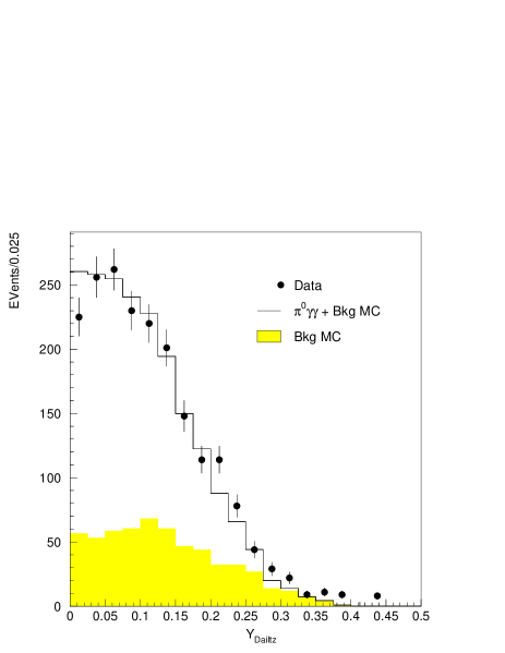
Figure 8: The $Y_{Dalitz}$ distribution for after all selection cuts. The dots show the data, the histogram the sum of the signal and background Monte Carlo simulation, and the shaded histogram the scaled background Monte Carlo simulation.

VII Systematic Uncertainties

In general, the systematic uncertainties related to the branching ratio measurement are associated with either the acceptance calculation or the background estimate. The largest systematic error is due to the change in the acceptance as a function of the value of $a_{V}$. This comes about mainly because the $m_{34}$ distribution depends upon the value of $a_{V}$, and the acceptance varies across the $m_{34}$ region. We find that the $a_{V}$ dependence has the following form: $B=(1.33+0.13\times a_{V})\times 10^{-6}$. We conservatively evaluate this systematic error by allowing $a_{V}$ to vary by $\pm 0.16$. The next largest systematic uncertainties are related to the acceptance ratio between the normalization and signal acceptances. To determine a systematic error for the acceptance, we compared the $K_{L}\to\pi^{0}\gamma\gamma$ data and Monte Carlo simulation. We then reweighted the specific Monte Carlo distribution to match the same distribution in data. We used this weight factor to calculate a new acceptance and used the difference to assign a systematic uncertainty. We also examined the $K_{L}\to\pi^{0}\pi^{0}$ decays and found similar results when reweighting the Monte Carlo simulation to match the data. Since the $K_{L}\to\pi^{0}\pi^{0}$ and $K_{L}\to\pi^{0}\gamma\gamma$ samples have nearly identical acceptances, this gives us confidence in our estimate in the systematic effects. The variables that had the largest effect on the acceptance were the kaon energy and the photon veto response. We assigned a systematic uncertainty of 1.16% due to the acceptance.

The ability of our Monte Carlo simulations to reproduce the $K_{L}\to\pi^{0}\pi^{0}\pi^{0}$ background also contributes to the systematic uncertainty. To estimate the effects from our knowledge of the background, we looked at all events before applying the shape $\chi^{2}$ cut. This sample is dominated by $K_{L}\to\pi^{0}\pi^{0}\pi^{0}$ events. We then reweighted the background Monte Carlo sample to match the data in a particular parameter. The change in acceptance multiplied by the background fraction was taken to be the systematic uncertainty from a specific variable. In particular, we assigned the following systematic uncertainties due to our simulation of the background: the photon shape $\chi^{2}$ (1.07%), the drift chamber simulation (0.92%), the photon veto simulation (0.90%), the kaon energy shape (0.69%), and the $K_{L}$ decay vertex distribution (0.38%).

In addition to the acceptance calculation and the background determination, a few other effects contribute to our systematic uncertainty including the Monte Carlo statistics, the background normalization and the measured $K_{L}\to\pi^{0}\pi^{0}$ and $\pi^{0}\to\gamma\gamma$ branching fractions. For this analysis, we generated nearly $10^{11}$ $K_{L}\to\pi^{0}\pi^{0}\pi^{0}$ decays, more than twice the background statistics. These statistics contribute 1.0% to the systematic uncertainty. To determine the normalization of the $K_{L}\to\pi^{0}\pi^{0}\pi^{0}$ Monte Carlo sample, we first scaled the $K_{L}\to\pi^{0}\pi^{0}$ Monte Carlo sample to the observed $\pi^{0}$ peak in the $m_{34}$ mass distribution in the data. We then normalized the $K_{L}\to\pi^{0}\pi^{0}\pi^{0}$ sample relative to the number of $K_{L}\to\pi^{0}\pi^{0}$ events by the ratio of the branching ratios and the number of generated events. To assign a background normalization systematic error, we scaled the $K_{L}\to\pi^{0}\pi^{0}\pi^{0}$ background events directly to the shape $\chi^{2}$ distribution and compared the difference between the two methods. This contribututed 0.90% to the total systematic uncertainty. Finally, we assigned a 0.5% systematic uncertaintly due to the error on the measured $K_{L}\to\pi^{0}\pi^{0}$ branching ratio. All of the systematic effects are listed in Table 2, with a total systematic uncertainty on the $K_{L}\to\pi^{0}\gamma\gamma$ branching ratio of 3.0%.

Type Source Uncertainty (%) Acceptance $a_{V}$ dependence 1.50 MC acceptance ratio 1.16 Background Photon shape $\chi^{2}$ 1.07 Drift chamber hits 0.92 Photon vetoes 0.90 Kaon energy 0.69 Decay Vertex 0.38 General MC statistics 1.00 Background normalization 0.90 $K_{L}\to 2\pi^{0}$ branching ratio 0.50 Total 3.0

Table 2: Branching ratio systematic uncertainties

To determine the systematic uncertainty in our $a_{V}$ measurement, we varied the position of the selection cuts and looked for any non-statistical change in the value of $a_{V}$. We also varied the level of $K_{L}\to\pi^{0}\pi^{0}\pi^{0}$ background according to the methods described above. The major systematic uncertainties associated with the determination of $a_{V}$ are listed in Table 3. The main sources of systematic error result from the uncertainty of the background estimations. The total systematic uncertainty associated with the $a_{V}$ measurement is 0.07.

Source	Uncertainty
Z vertex cut	0.05
Photon veto cut	0.04
3$\pi^{0}$ normalization	0.03
Photon shape $\chi^{2}$	0.01
Total	0.07

Table 3: $a_{V}$ fitting systematic uncertainty.

VIII Final Results and Conclusions

To obtain the final branching ratio result, we used the weighted average of the 1996-1997 and 1999 numbers based upon the statistical errors of the two results. The systematic studies were done on the combined 1997 and 1999 analyses to take into account any correlations. Including the uncertainties due to the systematic effects, we find the $K_{L}\to\pi^{0}\gamma\gamma$ branching ratio to be

$$B(K_{L} \to \pi^{0}\gamma\gamma)=$$ (3)

$$(1.29\pm 0.03_{stat}\pm 0.05_{syst})\times 10^{-6}.$$

This result is a significant improvement over the previous KTeV result, and supersedes that result. The differences between the current and previous results is discussed in Section IX.

Our value of $a_{V}$ was obtained using the fitting method described above. The $\chi^{2}$ for the fit is 56.6 for 59 degrees of freedom. Including the systematic error, we find

$$a_{V}=-0.31\pm 0.05_{stat}\pm 0.07_{syst}.$$ (4)

The total error from our determination of $a_{V}$ is slightly larger than the NA48 result, however, it is compatible with their value.

The branching ratio result is consistent with the latest $O(p^{6})$ ChPT results. Our value of $a_{V}$ suggests that the CP conserving amplitude in $K_{L}\to\pi^{0}l^{+}l^{-}$ should be less than $1\times 10^{-12}$ compared to the expected total branching ratio of $\sim 3\times 10^{-11}$ref:buchalla . Therefore this decay should be dominated by CP violating terms. Future searches for $K_{L}\to\pi^{0}e^{+}e^{-}$ and $K_{L}\to\pi^{0}\mu^{+}\mu^{-}$ would be of great interest since many models of new physics would signficantly alter these branching ratios.

IX Appendix A

Compared to the previous KTeV $K_{L}\to\pi^{0}\gamma\gamma$ branching ratio value, our new result is significantly lower. The main difference between the two analyses arises from our simulation of the transverse photon shower shape. Our previous analysis used the GEANT-based shower library, while our current analysis utilizes the data-based shower library. As shown in Figure 3, the data-based shower library shows significant improvement over the GEANT-based shower library. Utilizing this new shower library changes our estimate of the $K_{L}\to\pi^{0}\pi^{0}\pi^{0}$ background, increasing the background by a factor of approximately two. The increase in background occurs because the $K_{L}\to\pi^{0}\pi^{0}\pi^{0}$ background peaks in the region of small shape $\chi^{2}$ as shown in Figure 5. In our previous result the $K_{L}\to\pi^{0}\pi^{0}\pi^{0}$ background shape dropped in the signal region. Accordingly, the background estimate utilizing the GEANT-based shower library underestimated the $K_{L}\to\pi^{0}\pi^{0}\pi^{0}$ background.

In the previous result the systematic error for the mismatch in the photon shape $\chi^{2}$ scaled with the size of the estimated background. However, since the background shape was incorrectly modeled, our estimate of the systematic error also was underestimated. Studies of other variables sensitive to the $K_{L}\to\pi^{0}\pi^{0}\pi^{0}$ background arrive at a similar estimate for the background level in the current analysis.

- (1) G.D. Barr et al., Phys. Lett. B242, 523 (1990).
- (2) V. Papadimitriou et al., Phys. Rev. D44 R573 (1991).
- (3) G.D. Barr et al., Phys. Lett. B284, 440 (1992).
- (4) G. Ecker, A. Pich and E. de Rafael, Phys. Lett. B189, 363 (1987).
- (5) G. D’Ambrosio and J. Portoles, Nucl. Phys. B492, 417 (1997).
- (6) F. Gabbiani and G. Valencia, Phys. Rev D66, 074006 (2002).
- (7) T.N. Truong, Phys. Lett B313 221 (1993).
- (8) A. Alavi-Harati et al. Phys. Rev. Lett. 93 021805 (2004).
- (9) A. Alavi-Harati et al. Phys. Rev. Lett. 84 5279 (2000).
- (10) G. Buchalla, G. D’Ambrosio and G. Isidori, Nucl. Phys B672 387 (2003).
- (11) F. Mescia, C. Smith and S. Trine, JHEP 0608, 88 (2006).
- (12) J.R. Batley et al., Phys. Lett B576 43 (2003).
- (13) A. Alavi-Harati et al., Phys. Rev. Lett. 83, 917 (1999).
- (14) A. Lai et al., Phys. lett B536, 229 (2002).
- (15) A.Alavi-Harati et al., Phys. Rev D67, 012005 (2003).
- (16) A. Alavi-Harati et al., Phys. Rev D67, 012005 (2003).
- (17) C. Bown et al., Nucl. Instr. Meth. A369, 248, (1996).
- (18) R. Brun and F. Carminati, CERN Program Library Long Writeup W5013 (unpublished).
- (19) T. Alexopoulos et al., Phys. Rev D70, 092006 (2004).
- (20) W.-M. Yao et al., J. Phys G33, 1 (2006).
- (21) Data used to determine both the branching ratio and will be uploaded as an EPAPS document. For more information on EPAPS, see http://www.aip.org/pubservs/epaps.html.