Minor-Embedding in Adiabatic Quantum Computation: I. The Parameter Setting Problem

Abstract

We show that the NP-hard quadratic unconstrained binary optimization (QUBO) problem on a graph $G$ can be solved using an adiabatic quantum computer that implements an Ising spin-1/2 Hamiltonian, by reduction through minor-embedding of $G$ in the quantum hardware graph $U$. There are two components to this reduction: embedding and parameter setting. The embedding problem is to find a minor-embedding ${G_{\mathsf{emb}}}$ of a graph $G$ in $U$, which is a subgraph of $U$ such that $G$ can be obtained from ${G_{\mathsf{emb}}}$ by contracting edges. The parameter setting problem is to determine the corresponding parameters, qubit biases and coupler strengths, of the embedded Ising Hamiltonian. In this paper, we focus on the parameter setting problem. As an example, we demonstrate the embedded Ising Hamiltonian for solving the maximum independent set (MIS) problem via adiabatic quantum computation (AQC) using an Ising spin-1/2 system. We close by discussing several related algorithmic problems that need to be investigated in order to facilitate the design of adiabatic algorithms and AQC architectures.

1 Introduction

Adiabatic Quantum Computation (AQC) was proposed by Farhi et al.[15, 14] in 2000. The AQC model is based on the adiabatic theorem (see, e.g. [22]). Informally, the theorem says that if we take a quantum system whose Hamiltonian “slowly” changes from ${\mathcal{H}}_{\mathsf{init}}$ (initial Hamiltonian) to ${\mathcal{H}}_{\mathsf{final}}$ (final Hamiltonian), then if we start with the system in the groundstate (eigenvector corresponding to the lowest eigenvalue) of ${\mathcal{H}}_{\mathsf{init}}$, then at the end of the evolution the system will be “predominantly” in the ground state of ${\mathcal{H}}_{\mathsf{final}}$. The theorem is used to construct adiabatic algorithms for optimization problems in the following way: The initial Hamiltonian ${\mathcal{H}}_{\mathsf{init}}$ is designed such that the system can be readily initialized into its known groundstate, while the groundstate of the final Hamiltonian ${\mathcal{H}}_{\mathsf{final}}$ encodes the answer to the desired optimization problem. The complete (or system) Hamiltonian at a time $t$ is then given by

$${\mathcal{H}}(t)=\biggl{(}1-s(\frac{t}{T})\biggr{)}{\mathcal{H}}_{\mathsf{init}}+s(\frac{t}{T}){\mathcal{H}}_{\mathsf{final}}$$

for $t\in[0,T]$ where $s$ increases monotonically from $s(0)=0$ to $s(1)=1$ and $T$ is the total running time of the algorithm. If $T$ is large enough, which is determined by the minimum spectral gap (the difference between the two lowest energy levels) of the system Hamiltonian, the adiabatic theorem guarantees the state at time $t$ will be the groundstate of ${\mathcal{H}}(t)$, leading to the solution, the ground state of ${\mathcal{H}}(T)={\mathcal{H}}_{\mathsf{final}}$.

It is believed that AQC is advantageous over standard (the gate model) quantum computation in that it is more robust against environmental noise [11, 3, 4]. In 2004, D-Wave Systems Inc. undertook the endeavor to build an adiabatic quantum computer for solving NP-hard problems. Kaminsky and Lloyd [17] proposed a scalable architecture for AQC of NP-hard problems. Note that AQC is polynomially equivalent to the standard quantum computation, and therefore AQC is universal. Farhi et al. in their original paper [15] showed that AQC can be efficiently simulated by standard quantum computers. In 2004, Aharonov et al [1] proved the more difficult converse statement that standard quantum computation can be efficiently simulated by AQC. In this paper, however, we will focus on a subclass of Hamiltonians, known as Ising models in a transverse field, that are NP-hard but not universal for quantum computation. This subclass of Hamiltonians has been implemented by D-Wave Systems Inc.

D-Wave’s quantum hardware architecture can be viewed as an undirected graph $U$ with weighted vertices and weighted edges. See Figure 1 for an example.

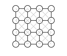
Figure 1: An example hardware graph: a $4\times 4$ extended grid. Each qubit is coupled with its nearest and next-nearest neighbors.

Denote the vertex set of $U$ by ${\mathsf{V}}(U)$ and the edge set of $U$ by ${\mathsf{E}}(U)$. Each vertex $i\in{\mathsf{V}}(U)$ corresponds to a qubit, and each edge $ij\in{\mathsf{E}}(U)$ corresponds to a coupler between qubit $i$ and qubit $j$. In the following, we will use qubit and vertex, and coupler and edge interchangeably when there is no confusion. There are two weights, $h_{i}$ (called the qubit bias) and $\Delta_{i}$ (called the tunneling amplitude), associated with each qubit $i$. There is a weight $J_{ij}$ (called the coupler strength) associated with each coupler $ij$. In general, these weights are functions of time, i.e., they vary over the time, e.g., $h_{i}(t)$.

The Hamiltonian of the Ising model in a transverse field thus implemented is:

$${\mathcal{H}}(t)=\sum_{i\in{\mathsf{V}}(G)}h_{i}(t)\sigma^{z}_{i}+\sum_{ij\in{\mathsf{E}}(G)}J_{ij}(t)\sigma^{z}_{i}\sigma^{z}_{j}+\sum_{i\in{\mathsf{V}}(G)}\Delta_{i}(t)\sigma^{x}_{i}$$

with $\sigma_{i}^{z}=I\otimes I\otimes\ldots\otimes\sigma^{z}\otimes\ldots\otimes I$ (the $\sigma^{z}$ is in the $i$th position), similarly for $\sigma^{x}_{i}$ and $\sigma^{z}_{i}\sigma^{z}_{j}$, where $I$ is the $2\times 2$ identity matrix, while $\sigma^{z}$ and $\sigma^{x}$ are the Pauli matrices given by

$$\sigma^{z}=\begin{bmatrix}1&0\\ 0&-1\end{bmatrix},\quad\text{and}\quad\sigma^{x}=\begin{bmatrix}0&1\\ 1&0\end{bmatrix}.$$

In general, the transverse field (i.e. $\sum_{i\in{\mathsf{V}}(G)}\Delta_{i}\sigma^{x}_{i}$) encodes the initial Hamiltonian ${\mathcal{H}}_{\mathsf{init}}$, while the other two terms encode the final Hamiltonian:

$${\mathcal{H}}_{\mathsf{final}}=\sum_{i\in{\mathsf{V}}(G)}h_{i}\sigma^{z}_{i}+\sum_{ij\in{\mathsf{E}}(G)}J_{ij}\sigma^{z}_{i}\sigma^{z}_{j}.$$ (1)

One can show (see Appendix) that the eigenvalues and the corresponding eigenstates of ${\mathcal{H}}_{\mathsf{final}}$ are encoded in the following energy function of Ising Model:

$${\mathcal{E}}(s_{1},\ldots,s_{n})=\sum_{i\in{\mathsf{V}}(G)}h_{i}s_{i}+\sum_{ij\in{\mathsf{E}}(G)}J_{ij}s_{i}s_{j}$$ (2)

where $s_{i}\in\{-1,+1\}$, called a spin, and $h_{i},J_{ij}\in{\mathbb{R}}$. In particular, the smallest eigenvalue of ${\mathcal{H}}_{\mathsf{final}}$ corresponding to the minimum of ${\mathcal{E}}$, and $\operatornamewithlimits{arg\ min}{\mathcal{E}}$ corresponds to its eigenvector (called ground state) of ${\mathcal{H}}_{\mathsf{final}}$. When there is no confusion, we use the energy function of Ising model and Ising Hamiltonian interchangeably. Hereafter, we refer the problem of finding the minimum energy of the Ising Model or equivalently the groundstate of Ising Hamiltonian as the Ising problem. It can be shown that the Ising problem is equivalent to the problem of Quadratic Unconstrained Boolean Optimization (QUBO)(see [9] and references therein), which has been shown to be a common model for a wide variety of discrete optimization problems. More specifically, finding the minimum of ${\mathcal{E}}$ in (2) is equivalent to finding the maximum of the following function (which is also known as quadratic pseudo-Boolean function [8]) of QUBO on the same graph:

$${\mathcal{Y}}(x_{1},\ldots,x_{n}) = \sum_{i\in{\mathsf{V}}(G)}c_{i}x_{i}-\sum_{ij\in{\mathsf{E}}(G)}J_{ij}x_{i}x_{j}$$ (3)

where $x_{i}\in\{0,1\}$, $c_{i},J_{ij}\in{\mathbb{R}}$. The correspondence between the parameters, $h$s and $c$s will be shown in Section 2. Therefore, given an Ising/QUBO problem on graph $G$, one can thus solve the problem on an adiabatic quantum computer (using an Ising spin-1/2 system) if $G$ can be embedded as a subgraph of the quantum hardware graph $U$. We refer this embedding problem as subgraph-embedding, to be defined formally in Section 3. In general, there are physical constraints on the hardware graph $U$. In particular, there is a degree-constraint in that each qubit can have at most a constant number of couplers dictated by hardware design. Therefore, besides the possible difficulty of the subgraph-embedding problem, the graphs that can be solved on a given hardware graph $U$ through subgraph-embedding must also be degree-bounded. Kaminsky et al. [17, 18] observed and proposed that one can embed $G$ in $U$ through ferromagnetic coupling “dummy vertices” to solve Maximum Independent Set (MIS) problem of planar cubic graphs (regular graphs of degree-3) on an adiabatic quantum computer. In particular, they proposed an $n\times n$ square lattice as a scalable hardware architecture on which all $n/3$-vertex planar cubic graphs are embeddable. The notion of embedding here follows naturally from physicists’ intuition that each logical qubit (corresponding to a vertex in the input graph) is mapped to a subtree of physical qubits (corresponding to vertices in the hardware graph) that are ferromagnetically coupled such that each subtree of physical qubits acts like a single logical qubit. For example, in Figure 2, the logical qubit $1$ (in orange color) of the graph $G$ is mapped to a subtree of physical qubits (labelled $1$) of the square lattice.

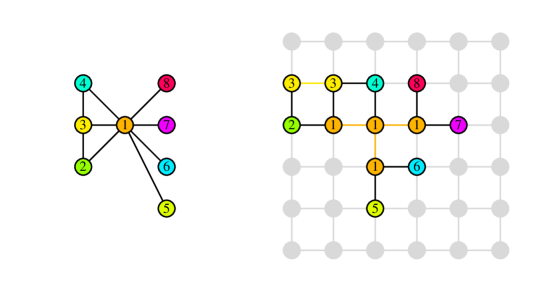
$G$                                                                  ${G_{\mathsf{emb}}}$

Figure 2: ${G_{\mathsf{emb}}}$(right) is a minor-embedding of $G$(left) in the square lattice $U$. Each vertex (called a logical qubit) of $G$ is mapped to a (connected) subtree of (same color/label) vertices (called physical qubits) of $U$. $G$ is called a (graph) minor of $U$.

Informally, a minor-embedding ${G_{\mathsf{emb}}}$ of a graph $G$ in the hardware graph $U$ is a subgraph of $U$ such that ${G_{\mathsf{emb}}}$ is an “expansion” of $G$ by replacing each vertex of $G$ with a (connected) subtree of $U$, or equivalently, $G$ can be obtained from ${G_{\mathsf{emb}}}$ by contracting edges (same color in Figure 2). In graph theory, $G$ is called a (graph) minor of $U$ (see for example [12]). The minor-embedding will be formally defined in Section 3. (Remark: The embedding in [17, 18] is a special case of minor-embedding, known as topological-minor embedding.)

By reduction through minor-embedding, we mean that one can reduce the original Ising Hamiltonian on the input graph $G$ to the embedded Ising Hamiltonian ${\mathcal{H}}^{{\mathsf{emb}}}$ on its minor-embedding ${G_{\mathsf{emb}}}$, i.e., the solution to the embedded Ising Hamiltonian gives rise to the solution to the original Ising Hamiltonian. The intuition suggests that the reduction will be correct provided that the ferromagnetic coupler strengths used are sufficiently strong (i.e., large negative number). However, how strong is “strong enough”? In [17, 18], they do not address this question, i.e. what are the required strengths of these ferromagnetic couplers? In Section 4.1, we will show that it is not difficult to give an upper bound for the ferromagnetic coupler strengths and thus explain the intuition. However, there are indications [2] that too strong ferromagnetic coupler strengths might slow down the adiabatic algorithm. Furthermore, an adiabatic quantum computer is an analog computer and analog parameters can only be set to a certain degree of precision (a condition much more stringent than the setting of digital parameters). Hence, the allowed values of coupler strengths are limited. Therefore, from the computational point of view, it is important to derive as small (in terms of magnitude) as possible sufficient condition for these ferromagnetic coupler strengths. Furthermore, what should the bias for physical qubits be?

There are two components to the reduction: embedding and parameter setting. The embedding problem is to find a minor-embedding ${G_{\mathsf{emb}}}$ of a graph $G$ in $U$. This problem is interdependent of the hardware graph design problem, which will be discussed in Section 6. The parameter setting problem is to set the corresponding parameters, qubit bias and coupler strengths, of the embedded Ising Hamiltonian. In this paper, we assume that the minor-embedding ${G_{\mathsf{emb}}}$ is given, and focus on the parameter setting problem (of the final Hamiltonian). Note that there are two aspects of efficiency of a reduction. One is how efficient one can reduce the original problem to the reduced problem. For example, here we are concerned how efficiently we can compute the minor-embedding and how efficiently we can compute the new parameters of the embedded Ising Hamiltonian. The other aspect concerns about the efficiency (in terms the running time) of the adiabatic algorithm for the reduced problem. In general, the latter depends on the former. For example, the running time of the adiabatic algorithm may depend on a “good” embedding that is reduced to. According to the adiabatic theorem (see, e.g. [22]), the running time of the adiabatic algorithm depends on the minimum spectral gap (the difference between the two lowest energy levels) of the system Hamiltonian, which is defined by both initial Hamiltonian and final Hamiltonian. That is, the running time (and thus the efficiency of the reduction) will depend on both the initial Hamiltonian and the final Hamiltonian. In this paper, our focus is only on the final Hamiltonian, and therefore we are not able to address the running time of the adiabatic algorithm. Furthermore, the estimation of the minimum spectral gap of the (system) Hamiltonian is in general hard. Consequently, analytically analyzing the running time of an adiabatic algorithm is in general an open question.

Finally, let us remark that there is another different approach based on perturbation theory by Oliveira & Terhal [21] for performing the reduction. In particular, they employed perturbative gadgets to reduce a 2-local (system) Hamiltonian to a 2-local Hamiltonian on a 2-D square lattice, and were able to show (as in the pioneering work [19]) that the minimum spectral gap (and thus the running time) of the system Hamiltonian is preserved (up to a polynomial factor) after the reduction, for any given initial Hamiltonian. However, besides the ineffective embedding, as pointed out in [10], the method is “unphysical” as it requires that each parameter grows with the system size.

The rest of the paper is organized as follows. In Section 2, we recall the equivalences between the QUBO problem and the Ising problem. In Section 3, we introduce the minor-embedding definition and mention related work in graph theory. In Section 4, we derive the new parameters, namely values for the qubit bias and the sufficient condition for the ferromagnetic coupler strengths, for the embedded Ising Hamiltonian such that the original Ising problem can be correctly solved through the embedded Ising problem. In Section 5, we show the embedded Ising Hamiltonian for solving the (weighted) MIS problem. Finally, we conclude with several related algorithmic problems that need to be investigated in order to facilitate the design of efficient adiabatic algorithms and AQC architectures in Section 6.

2 Equivalences Between QUBO and the Ising Problem

In this section, we recall the equivalences between the problem of QUBO (maximization of ${\mathcal{Y}}$ in Eq. (3)) and the Ising problem (minimization of ${\mathcal{E}}$ in Eq. (2)). Notice that $x_{i}=\frac{s_{i}+1}{2}$, that is, $x_{i}=1$ corresponds to $s_{i}=1$, and $x_{i}=0$ corresponds to $s_{i}=-1$. Using a change of variables, we have

$${\mathcal{Y}}(x_{1},\ldots,x_{n}) = \frac{1}{2}\sum_{i\in{\mathsf{V}}(G)}c_{i}-\frac{1}{4}\sum_{ij\in{\mathsf{E}}(G)}J_{ij}-\frac{1}{4}\left(\sum_{i\in{\mathsf{V}}(G)}\left(\sum_{j\in{\mathsf{nbr}}(i)}J_{ij}-2c_{i}\right)s_{i}+\sum_{ij\in{\mathsf{E}}(G)}J_{ij}s_{i}s_{j}\right)$$

where ${\mathsf{nbr}}(i)\stackrel{{\scriptstyle\mathrm{def}}}{{=}}\{j:ij\in{\mathsf{E}}(G)\}$, the neighborhood of vertex $i$, for $i\in{\mathsf{V}}(G)$.

Therefore, $\mathsf{Max}{\mathcal{Y}}(x_{1},\ldots,x_{n})$ in Eq. (3) is equivalent to $\mathsf{Min}{\mathcal{E}}(s_{1},\ldots,s_{n})$ in Eq. (2) where $h_{i}=\sum_{j\in{\mathsf{nbr}}(i)}J_{ij}-2c_{i}$, or $c_{i}=1/2(\sum_{j\in{\mathsf{nbr}}(i)}J_{ij}-h_{i})$ for $i\in{\mathsf{V}}(G)$. See Figure 4 for the correspondences between parameters in QUBO and the Ising model.

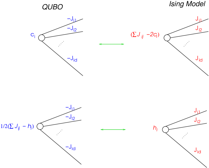
Figure 3: The correspondences between the parameters in QUBO and the Ising Model.

3 Minor-Embedding

Definition 3.1.

Let $U$ be a fixed hardware graph. Given $G$, the minor-embedding of $G$ is defined by

$$\phi:G\longrightarrow U$$

such that

• each vertex in ${\mathsf{V}}(G)$ is mapped to a connected subtree $T_{i}$ of $U$;

• there exists a map $\tau:{\mathsf{V}}(G)\times{\mathsf{V}}(G)\longrightarrow{\mathsf{V}}(U)$ such that for each $ij\in{\mathsf{E}}(G)$, there are corresponding $i_{\tau(i,j)}\in{\mathsf{V}}(T_{i})$ and $j_{\tau(j,i)}\in{\mathsf{V}}(T_{j})$ with $i_{\tau(i,j)}j_{\tau(j,i)}\in{\mathsf{E}}(U)$.

Given $G$, if $\phi$ exists, we say that $G$ is embeddable in $U$. In graph theory, $G$ is called a minor of $U$. When $\phi$ is clear from the context, we denote the minor-embedding $\phi(G)$ of $G$ by ${G_{\mathsf{emb}}}$.

Equivalently, one can think of a minor $G$ of $U$ as a graph that can be obtained from a subgraph of $U$ by contracting edges. See Figure 2 for an example.

In particular, there are two special cases of minor-embedding:

• Subgraph-embedding: Each $T_{i}$ consists of a single vertex in $U$. That is, $G$ is isomorphic to ${G_{\mathsf{emb}}}$ (a subgraph of $U$).

• Topological-minor-embedding: Each $T_{i}$ is a chain (or path) of vertices in $U$.

Minors are well-studied in graph theory, see for example [12]. Given a fixed graph $G$, there are algorithms that find a minor-embedding of $G$ in $U$ in polynomial time of size of $U$, from the pioneering $O(|{\mathsf{V}}(U)|^{3})$ time algorithm by Robertson and Seymour [23] to recent nearly linear time algorithm of B. Reed (not yet published). However, it is worthwhile to reiterate that these algorithms are for fixed $G$, and their running times are exponential in the size of $G$. Here the minor-embedding problem is to find a minor-embedding of $G$ (for any given $G$) while fixing $U$. To the best of our knowledge, the only known work related to our minor-embedding problem was by Kleinberg and Rubinfeld [20], in which they showed that there is a randomized polynomial algorithm, based on a random walk, to find a minor-embedding in a given degree-bounded expander.

Our embedding problem might appear similar to the embedding problem from parallel architecture studies. However, besides the different physical constraints for the design of architectures, the requirements are very different. In particular, in our embedding problem, we do not allow for load $>1$, which is the maximum number of logical qubits mapped to a single physical qubit. Also, we require dilation, which is the maximum number of stretched edges (through other qubits), to be exactly 1. However, all of the existing research on embedding problems for parallel processors [13], at least one of the conditions is violated (namely either load $>1$ or dilation $>1$). In this paper, our focus is on parameter setting such that the reduction is correct, and not on the minor-embedding algorithm and/or the related (minor-universal) hardware graph $U$ design. These problems will be addressed in a subsequent paper.

4 Parameter Requirement for the Embedded Ising Hamiltonian

Let the QUBO problem, specified by ${\mathcal{Y}}$ and $G$, be given as in Eq.(3), and the corresponding ${\mathcal{E}}$ in Eq.(2). Suppose ${G_{\mathsf{emb}}}$ is a minor-embedding of $G$, and let ${\mathcal{E}}^{{\mathsf{emb}}}$ be the embedded energy function associated with ${G_{\mathsf{emb}}}$:

$${\mathcal{E}}^{{\mathsf{emb}}}(s_{1},\ldots,s_{N}) = \sum_{i\in{\mathsf{V}}({G_{\mathsf{emb}}})}h^{\prime}_{i}s_{i}+\sum_{ij\in{\mathsf{E}}({G_{\mathsf{emb}}})}J^{\prime}_{ij}s_{i}s_{j}$$

where $|{\mathsf{V}}({G_{\mathsf{emb}}})|=N$.

Our goal is to find out the requirement for new parameters, $h^{\prime}$s and $J^{\prime}$s, such that one can solve the original Ising problem on $G$ by solving the embedded Ising problem on its embedding ${G_{\mathsf{emb}}}$, or equivalently, such that there is an one-one correspondence between the minimum of ${\mathcal{E}}$ (and thus the maximum of ${\mathcal{Y}}$) and the minimum of ${\mathcal{E}}^{{\mathsf{emb}}}$.

As we mentioned in the introduction, the idea that we can solve the original Ising problem (i.e. finding the groundstate of the Ising Hamiltonian) on the input graph $G$ by solving the new Ising problem on the embedded graph ${G_{\mathsf{emb}}}$ in $U$ is that one can use ferromagnetic couplers to connect the physical qubits in each $T_{i}$ of ${G_{\mathsf{emb}}}$ such that the subtree $T_{i}$ will act as one logical qubit $i$ of $G$.

Notation.

First, we recall that ${\mathsf{V}}({G_{\mathsf{emb}}})=\bigcup_{i\in{\mathsf{V}}(G)}{\mathsf{V}}(T_{i})$ and ${\mathsf{E}}({G_{\mathsf{emb}}})=\bigcup_{i\in{\mathsf{V}}(G)}{\mathsf{E}}(T_{i})\cup\bigcup_{ij\in{\mathsf{E}}(G)}i_{\tau(i,j)}j_{\tau(j,i)}.$ We distinguish the edges within $T_{i}$s from the edges corresponding to the edges in the original graph. Denote the latter by ${\mathsf{OE}}({G_{\mathsf{emb}}})$, that is, ${\mathsf{OE}}({G_{\mathsf{emb}}})=\bigcup_{ij\in{\mathsf{E}}(G)}i_{\tau(i,j)}j_{\tau(j,i)}$. (The black edges in ${G_{\mathsf{emb}}}$ of Figure 2 correspond to ${\mathsf{OE}}({G_{\mathsf{emb}}})$.) For convenience, ${\mathsf{Onbr}}(i_{k})\stackrel{{\scriptstyle\mathrm{def}}}{{=}}{\mathsf{nbr}}(i_{k})\cap{\mathsf{OE}}({G_{\mathsf{emb}}})$ and ${\mathsf{Fnbr}}(i_{k})\stackrel{{\scriptstyle\mathrm{def}}}{{=}}{\mathsf{nbr}}(i_{k})\setminus{\mathsf{Onbr}}(i_{k})$, $i_{k}\in{\mathsf{V}}(T_{i})$. Note $j_{\tau(j,i)}\in{\mathsf{Onbr}}(i_{k})\Leftrightarrow ij\in{\mathsf{E}}(G)$.

The above intuition suggests that we use the same coupler strength for each original edge, i.e., $J^{\prime}_{i_{\tau(i,j)}j_{\tau(j,i)}}=J_{ij}$ for ${i_{\tau(i,j)}j_{\tau(j,i)}}\in{\mathsf{OE}}({G_{\mathsf{emb}}})$, and use ferromagnetic coupler strength, $F_{i}^{e}(<0)$, for each edge $e\in{\mathsf{E}}(T_{i})$, and redistribute the bias $h_{i}$ of a logical qubit $i$ to its physical qubits in $T_{i}$. That is, we choose $h^{\prime}_{i_{k}}$ for physical qubit $i_{k}\in{\mathsf{V}}(T_{i})$ such that $\sum_{{i_{k}}\in{\mathsf{V}}(T_{i})}h^{\prime}_{i_{k}}=h_{i}$.

Therefore, we have

$${\mathcal{E}}^{{\mathsf{emb}}}(s_{1},\ldots,s_{N}) = \sum_{i\in{\mathsf{V}}(G)}\left(\sum_{i_{k}\in{\mathsf{V}}(T_{i})}h^{\prime}_{i_{k}}s_{i_{k}}+\sum_{i_{p}i_{q}\in{\mathsf{E}}(T_{i})}F_{i}^{pq}s_{i_{p}}s_{i_{q}}\right)+\sum_{ij\in{\mathsf{E}}(G)}J_{ij}s_{i_{\tau(i,j)}}s_{j_{\tau(j,i)}}$$ (4)

4.1 An Easy Upper Bound for the Ferromagnetic Coupler Strengths

In this section, we derive an easy upper bound for the ferromagnetic coupler strengths. The derivation is based on the penalty or multiplier method, in which a constrained optimization is reduced to an unconstrained one by replacing the corresponding expression into the objective function as a penalty term with a large multiplier. For example, this was used in the reduction from general (higher-order) unconstrained binary optimization to the quadratic one (see [8]).

Notice that by construction (i.e., $G$ is a minor of ${G_{\mathsf{emb}}}$ and $h^{\prime}_{i_{k}}$s are chosen such that $\sum_{{i_{k}}\in{\mathsf{V}}(T_{i})}h^{\prime}_{i_{k}}=h_{i}$), minimization of ${\mathcal{E}}$ in (2) is equivalent to

$$\min{\mathcal{E}}_{\mathsf{constrained}}(s_{1},\ldots,s_{N}) = \sum_{i\in{\mathsf{V}}(G)}\sum_{i_{k}\in{\mathsf{V}}(T_{i})}h^{\prime}_{i_{k}}s_{i_{k}}+\sum_{ij\in{\mathsf{E}}(G)}J_{ij}s_{i_{\tau(i,j)}}s_{j_{\tau(j,i)}}$$ (5)

subject to

$$s_{i_{p}}s_{i_{q}} = 1\mbox{ for all }i_{p}i_{q}\in{\mathsf{E}}(T_{i}),i\in{\mathsf{V}}(G)$$

where the condition $s_{i_{p}}s_{i_{q}}=1$ for all $i_{p}i_{q}\in{\mathsf{E}}(T_{i})$ is equivalent to requiring the spins of physical qubits that correspond to the same logical qubit $i$ to be of the same sign.

The corresponding unconstrained minimization is thus

$$\min{\mathcal{E}}^{\prime}(s_{1},\ldots,s_{N}) = \sum_{i\in{\mathsf{V}}(G)}\sum_{i_{k}\in{\mathsf{V}}(T_{i})}\left(h^{\prime}_{i_{k}}s_{i_{k}}+\sum_{i_{p}i_{q}\in{\mathsf{E}}(T_{i})}F_{i}^{pq}(s_{i_{p}}s_{i_{q}}-1)\right)+\sum_{ij\in{\mathsf{E}}(G)}J_{ij}s_{i_{\tau(i,j)}}s_{j_{\tau(j,i)}}$$ (6)

which is equivalent to solving Eq.(4) as $\sum_{i\in{\mathsf{V}}(G)}\sum_{i_{p}i_{q}\in{\mathsf{E}}(T_{i})}F_{i}^{pq}$ is a constant. We are interested in how large (in terms of magnitude) $F_{i}^{pq}$s are sufficient to guarantee that the solution of Eq.(6) gives the solution to Eq.(5), and consequently to Eq.(2). The result is stated in the following theorem.

Theorem 4.1.

Let ${\mathcal{E}}_{\mathsf{constrained}}$ and ${\mathcal{E}}^{\prime}$ given as in Eq.(5) and Eq.(6). Suppose that for $i\in{\mathsf{V}}(G)$,

$$F_{i}^{pq}<-\left(|h_{i}|+\sum_{j\in{\mathsf{nbr}}(i)}|J_{ij}|\right)~{}\quad\quad\text{ for }i_{p}i_{q}\in{\mathsf{E}}(T_{i})$$ (7)

then we have $s_{i_{p}}^{*}s_{i_{q}}^{*}=1\mbox{ for all }i_{p}i_{q}\in{\mathsf{E}}(T_{i})$, $i\in{\mathsf{V}}(G)$, where $(s_{1_{1}}^{*},\ldots,s_{N}^{*})=\operatornamewithlimits{arg\ min}{\mathcal{E}}^{\prime}$. Consequently,

$$\min{\mathcal{E}}_{\mathsf{constrained}}(s_{1},\ldots,s_{N})=\min{\mathcal{E}}^{\prime}(s_{1},\ldots,s_{N}).$$

Proof.

Let $(s_{1_{1}}^{*},\ldots,s_{N}^{*})=\operatornamewithlimits{arg\ min}{\mathcal{E}}^{\prime}.$ Suppose on the contrary. That is, there exists $f_{p}f_{q}\in{\mathsf{E}}(T_{f})$, for some $1\leq f\leq n$ such that $s_{f_{p}}^{*}s_{f_{q}}^{*}=-1$. Then we have

$${\mathcal{E}}^{\prime}(s_{1}^{*},\ldots,s_{N}^{*})\geq-\left(\sum_{f_{k}\in{\mathsf{V}}(T_{f})}|h^{\prime}_{f_{k}}|+\sum_{j\in{\mathsf{nbr}}(f)}|J_{fj}|\right)-2F_{f}^{pq}+{\mathcal{E}}^{\prime}_{\mathsf{rest}}(s_{1}^{*},\ldots,s_{N}^{*})$$

where

$${\mathcal{E}}^{\prime}_{\mathsf{rest}}(s_{1},\ldots,s_{N})=\sum_{i\in{\mathsf{V}}(G),i\neq f}\sum_{i_{k}\in{\mathsf{V}}(T_{i})}\left(h^{\prime}_{i_{k}}s_{i_{k}}+\sum_{i_{p}i_{q}\in{\mathsf{E}}(T_{i})}F_{i}^{pq}(s_{i_{p}}s_{i_{q}}-1)\right)+\sum_{ij\in{\mathsf{E}}(G),i\neq f}J_{ij}s_{i_{\tau(i,j)}}s_{j_{\tau(j,i)}}.$$

Thus, if $F$s satisfy Eq.(LABEL:eq:F-condition2), we have

$${\mathcal{E}}^{\prime}(s_{1}^{*},\ldots,s_{N}^{*})>\sum_{f_{k}\in{\mathsf{V}}(T_{f})}|h^{\prime}_{f_{k}}|+\sum_{j\in{\mathsf{nbr}}(f)}|J_{fj}|+{\mathcal{E}}^{\prime}_{\mathsf{rest}}(s_{1}^{*},\ldots,s_{N}^{*})$$

which is at least $\min{\mathcal{E}}^{\prime}(s_{1},\ldots,s_{N})={\mathcal{E}}^{\prime}(s_{1}^{*},\ldots,s_{N}^{*})$, a contradiction. Consequently, we can conclude that $s_{i_{p}}^{*}s_{i_{q}}^{*}=1\mbox{ for all }i_{p}i_{q}\in{\mathsf{E}}(T_{i})$, $i\in{\mathsf{V}}(G)$, where $(s_{1_{1}}^{*},\ldots,s_{N}^{*})=\operatornamewithlimits{arg\ min}{\mathcal{E}}^{\prime}$, implying the claimed equality of the minima. ∎

4.2 A Tighter Bound for the Ferromagnetic Coupler Strengths

As we mentioned Section 1, it is desired to obtain tighter bounds for the ferromagnetic coupler strengths. In this section, we show that with a more careful analysis, we can reduce the bound by setting the qubit bias ($h^{\prime}$) appropriately.

For $i\in{\mathsf{V}}(G)$, let

$$C_{i}\stackrel{{\scriptstyle\mathrm{def}}}{{=}}\sum_{j\in{\mathsf{nbr}}(i)}|J_{ij}|-|h_{i}|.$$

Observe that if $C_{i}<0$, that is, $\sum_{j\in{\mathsf{nbr}}(i)}|J_{ij}|<|h_{i}|$. Then we have $s_{i}^{*}=-1$ for $h_{i}>0$, and $s_{i}^{*}=+1$ for $h_{i}<0$, where $(s_{1}^{*},\ldots,s_{n}^{*})=\operatornamewithlimits{arg\ min}{\mathcal{E}}$. Therefore, WLOG, for the rest of the paper, we will assume that $C_{i}\geq 0$.

Theorem 4.2.

Let ${\mathcal{E}}$ (${\mathcal{Y}}$ resp.) and $G$ be given as in Eq.(2) (Eq.(3) resp.). Suppose ${G_{\mathsf{emb}}}$ is a minor-embedding of $G$, and let ${\mathcal{E}}^{{\mathsf{emb}}}$ be the energy of the embedded Ising Hamiltonian given in Eq.(4). Then for all $i\in{\mathsf{V}}(G)$, if

$$h^{\prime}_{i_{k}}=sign(h_{i})\left\{\begin{array}[]{ll}\sum_{j_{\tau(j,i)}\in{\mathsf{Onbr}}(i_{k})}|J_{ij}|-C_{i}/l_{i}&i_{k}\mbox{ is one of the $l_{i}$ leaves of }T_{i}\\ \sum_{j_{\tau(j,i)}\in{\mathsf{Onbr}}(i_{k})}|J_{ij}|&\mbox{ otherwise }\end{array}\right.$$

and

$$F_{i}^{e}<-\frac{l_{i}-1}{l_{i}}C_{i}~{}~{}\mbox{for all }e\in{\mathsf{E}}(T_{i}),$$

where $C_{i}\geq 0$ (defined above) and $sign(h_{i})=+1(-1$ resp.) if $h_{i}\geq 0$ ($h_{i}<0$ resp.), we have $s_{i_{p}}^{*}s_{i_{q}}^{*}=1\mbox{ for all }i_{p}i_{q}\in{\mathsf{E}}(T_{i})$, $i\in{\mathsf{V}}(G)$, where $(s_{1_{1}}^{*},\ldots,s_{N}^{*})=\operatornamewithlimits{arg\ min}{\mathcal{E}}^{{\mathsf{emb}}}$. Consequently, there is one-one correspondence between $\operatornamewithlimits{arg\ min}{\mathcal{E}}^{{\mathsf{emb}}}$ and $\operatornamewithlimits{arg\ min}{\mathcal{E}}$ (and thus $\operatornamewithlimits{arg\ max}{\mathcal{Y}}$).

Furthermore, if we set $F_{i}^{e}=-\frac{l_{i}-1}{l_{i}}C_{i}-g_{i}/2$, for some $g_{i}>0$, then the spectral gap (which is the difference between the two lowest energy levels) of the embedded Ising Hamiltonian will be the minimum of $\min_{i\in{\mathsf{V}}(G)}g_{i}$ and the spectral gap of the original Ising Hamiltonian.

See Figure 4 for an example of the corresponding parameters in the embedded Ising Hamiltonian (for the topological-minor-embedding case).

Figure 4: The corresponding parameters in the embedded Ising Model. Bottom right, for $J>0$; bottom left, for general $J$: $J_{i1}>0$, $J_{i2}<0,J_{i3}<0$, and $c_{i}^{\prime}=c_{i}-\sum_{j\in{\mathsf{nbr}}(i),J_{ij}<0}J_{ij}$.

In the following, we first explain the main idea behind, followed by the formal proof. For the illustration purpose, suppose $h_{i}>0$, consider the simplest case in which all but one leaf is $-1$. Now, consider the energy change if the leaf is flipping from $+1$ to $-1$. Our goal is to set $F$s as small (in terms of the magnitude) as possible, such that the energy change is at least greater than zero. Note that the energy change $\Delta{\mathcal{E}}_{i_{k}}=$ $2(h^{\prime}_{i_{k}}+\sum_{j\tau(i,j)\in{\mathsf{Onbr}}(i_{k})}\delta_{j_{\tau(j,i)}}J_{ij}-F)$ where $\delta_{j_{\tau(j,i)}}$ depends on the sign of spin $s_{j_{\tau(j,i)}}^{*}$. We would like to bound $\Delta{\mathcal{E}}_{i_{k}}$ without knowing the signs of $s_{j_{\tau(j,i)}}^{*}$s. Observe that if $J$s are all positive, then the worst case we have $\Delta{\mathcal{E}}_{i_{k}}\geq 2(h^{\prime}_{i_{k}}-\sum_{j_{\tau(i,j)}\in{\mathsf{Onbr}}(i_{k})}J_{ij}-F)$. And in general $\Delta{\mathcal{E}}_{i_{k}}\geq 2(h^{\prime}_{i_{k}}-\sum_{j_{\tau(i,j)}\in{\mathsf{Onbr}}(i_{k})}J_{ij}^{+}+\sum_{j_{\tau(i,j)}\in{\mathsf{Onbr}}(i_{k})}J_{ij}^{-}-F)$, where $J_{ij}^{+}>0$ and $J_{ij}^{-}<0$. Consequently, setting $F<h^{\prime}_{i_{k}}-\sum_{j_{\tau(i,j)}\in{\mathsf{Onbr}}(i_{k})}|J_{ij}|$ would imply $\Delta{\mathcal{E}}_{i_{k}}>0$. One can then extend this argument to a segment that needs to be flipped, as illustrated in Figure  5.

$$\begin{array}[]{cc}\includegraphics[width=216.81pt]{proof-sketch1.eps}&\includegraphics[width=216.81pt]{proof-sketch.eps}\\ (a)h>0:\Delta{\mathcal{E}}\geq 2(h-J^{+}-J^{+}-F)&(b)h>0:\Delta{\mathcal{E}}\geq 2(h-J^{+}+J^{-}-F)\\ \\ \includegraphics[width=216.81pt]{proof-sketch2.eps}&\includegraphics[width=216.81pt]{proof-sketch3.eps}\\ (c)h>0&(d)h<0\end{array}$$

Figure 5: $(a)$ For $h>0$ and positive $J$s (denoted by $J^{+}$), the energy change $\Delta{\mathcal{E}}\geq 2(h-J^{+}-J^{+}-F)$ when flipping the leaf’s spin from $+1$ to $-1$. $(b)$ For $h>0$, $\Delta{\mathcal{E}}\geq 2(h-J^{+}+J^{-}-F)$ when flipping the leaf’s spin from $+1$ to $-1$, where $J^{+}>0$, $J^{-}<0$. (c) For $h>0$, flip a segment from $+1$ to $-1$. (d) For $h<0$, flip a segment from $-1$ to $+1$.

Proof.

It is easy to check that $\sum_{i_{k}\in{\mathsf{V}}(T_{i})}h^{\prime}_{i_{k}}=sign(h_{i})|h_{i}|=h_{i}$.

We will first prove the theorem when ${G_{\mathsf{emb}}}$ is a topological-minor-embedding of $G$. That is, each $T_{i}$ is a chain $(i_{1},i_{2},\ldots,i_{t_{i}})$ connected by consecutive vertices. Thus, the corresponding embedded energy function is given by

$${\mathcal{E}}^{{\mathsf{emb}}}(s_{1},\ldots,s_{N}) = \sum_{i\in{\mathsf{V}}(G)}\left(\sum_{k=1}^{t_{i}}h^{\prime}_{i_{k}}s_{i_{k}}+\sum_{k=1}^{t_{i}-1}F_{i}^{k(k+1)}s_{i_{k}}s_{i_{k+1}}\right)+\sum_{ij\in{\mathsf{E}}(G)}J_{ij}s_{i_{\tau(i,j)}}s_{j_{\tau(j,i)}}$$ (8)

In this case, we have $l_{i}=2$. We prove by contradiction. Suppose NOT. That is, there exists $i\in{\mathsf{V}}(G)$, and $1\leq k<t_{i}$ such that $s_{i_{k}}^{*}s_{i_{k+1}}^{*}=-1$. We distinguish two cases based on the value of $h_{i}$.

For $h_{i}>0$, let $p$ be the smallest index such that $s_{i_{p-1}}^{*}=-1$ and $s_{i_{p}}^{*}=+1$, and let $q$ be the smallest index such that $s_{i_{q}}^{*}=+1$ and $s_{i_{q+1}}^{*}=-1$. That is, we have $s_{i_{1}}^{*}=\ldots=s_{i_{p-1}}^{*}=-1$, $s_{i_{p}}^{*}=\ldots=s_{i_{q}}^{*}=+1$. Note we have at least either $p>1$ or $q<n$. (Otherwise they are all $+1$). Then we claim that by flipping the segment $(i_{p},\ldots,i_{q})$ from $+1$s to $-1$s, the energy decreases, contradicting to the optimality. (Notice that the $F$s within the segment do not change.) The energy change equals to

$$\Delta{\mathcal{E}}^{{\mathsf{emb}}} = {\mathcal{E}}^{{\mathsf{emb}}}(\ldots,-1,\ldots,-1,\underbrace{+1,\ldots,+1},-1,\ldots)-{\mathcal{E}}^{{\mathsf{emb}}}(\ldots,-1,\ldots,-1,\underbrace{-1,\ldots,-1},-1,\ldots)$$

$$\geq 2\left(\sum_{k=p}^{q}h^{\prime}_{i_{k}}-\sum_{k=p}^{q}\sum_{j_{\tau(j,i)}\in{\mathsf{Onbr}}(i_{k})}|J_{ij}|-F_{i}^{(p-1)p}-F_{i}^{q(q+1)}\right)\mbox{ (with convention that $F_{i}^{01}=F_{i}^{t_{i}(t_{i}+1)}=0$)}$$

References

- [1] D. Aharonov, W. van Dam, J. Kempe, Z. Landau, S. Lloyd, and O. Regev. Adiabatic quantum computation is equaivalent to standard quantum computation. Proc. 45th FOCS, pages 42–51, 2004.
- [2] M. H. S. Amin and V. Choi. Work in progress. 2008.
- [3] M. H. S. Amin, P. J. Love, and C. J. S. Truncik. Thermally assisted adiabatic quantum computation. Physical Review Letters, 100:060503, 2008.
- [4] M. H. S. Amin, C. J. S. Truncik, and D. V. Averin. The role of single qubit decoherence time in adiabatic quantum computation. arXiv.org:0803.1196.
- [5] B. S. Baker. Approximation algorithms for NP-complete problems on planar graphs. J. ACM, 41(1):153–180, 1994.
- [6] N. Bansal, S. Bravyi, and B. M. Terhal. A classical approximation scheme for the ground-state energy of Ising spin hamiltonians on planar graphs. quant-ph/0705.1115.
- [7] F. Barahona. On the computational complexity of Ising spin glass models. J. Phys. A: Math. Gen., pages 15: 3241–3253, 1982.
- [8] E. Boros and P. Hammer. Pseudo-boolean optimization. Discrete Appl. Math., (123):155–225, 2002.
- [9] E. Boros, P. L. Hammer, and G. Tavares. Preprocessing of quadratic unconstrained binary optimization. Technical Report RRR 10-2006, RUTCOR Research Report., 2006.
- [10] S. Bravyi, D. P. DiVincenzo, D. Loss, and B. M. Terhal. Simulation of many-body hamiltonians using perturbation theory with bounded-strength interactions. arXiv.org:0803.2686.
- [11] A. Childs, E. Farhi, and J. Preskill. Robustness of adiabatic quantum computation. Physical Review A, 65, 2002.
- [12] R. Diestel. Graph Theory. Springer-Verlag, Heidelberg, 2005.
- [13] L. F. Thomson. Introduction to parallel algorithms and architectures: arrays, trees, hypercubes. 1992.
- [14] E. Farhi, J. Goldstone, S. Gutmann, J. Lapan, A. Lundgren, and D. Preda. A quantum adiabatic evolution algorithm applied to random instances of an np-complete problem. Science, 292(5516):472–476, 2001.
- [15] E. Farhi, J. Goldstone, S. Gutmann, and M. Sipser. Quantum computation by adiabatic evolution. quant-ph/0001106, 2000.
- [16] L. M. Ioannou and M. Mosca. Limitations of some simple adiabatic quantum algorithms. quant-ph/0702241, 2007.
- [17] W. M. Kaminsky and S. Lloyd. Scalable architecture for adiabatic quantum computing of NP-hard problems. In A. J. Leggett, B. Ruggiero, and P. Silvestrini, editors, Quantum Computing and Quantum Bits in Mesoscopic Systems, 2004.
- [18] W. M. Kaminsky, S. Lloyd, and T. P. Orlando. Scalable superconducting architecture for adiabatic quantum computation. arXiv.org:quant-ph/0403090, 2004.
- [19] J. Kempe, A. Kitaev, and O. Regev. The complexity of the local hamiltonian problem. SIAM JOURNAL OF COMPUTING, 35:1070, 2006.
- [20] J. M. Kleinberg and R. Rubinfeld. Short paths in expander graphs. In IEEE Symposium on Foundations of Computer Science, pages 86–95, 1996.
- [21] R. Oliveira and B. M. Terhal. The complexity of quantum spin systems on a two-dimensional square lattice. quant-ph/0504050.
- [22] B. W. Reichardt. The quantum adiabatic optimization algorithm and local minima. In STOC ’04: Proceedings of the thirty-sixth annual ACM symposium on Theory of computing, pages 502–510, New York, NY, USA, 2004. ACM.
- [23] N. Robertson and P. D. Seymour. Graph minors. xiii: the disjoint paths problem. J. Comb. Theory Ser. B, 63(1):65–110, 1995.
- [24] W. van Dam, M. Mosca, and U. Vazirani. How powerful is adiabatic quantum computation? Proc. 42nd FOCS, pages 279–287, 2001.
- [25] W. van Dam and U. Vazirani. Limits on quantum adiabatic optimization. Unpublished, 2001.
Appendix