Perturbative study of the Kitaev model with spontaneous time-reversal symmetry breaking

Abstract

We analyze the Kitaev model on the triangle-honeycomb lattice whose ground state has recently been shown to be a chiral spin liquid. We consider two perturbative expansions : the isolated-dimer limit containing Abelian anyons and the isolated-triangle limit. In the former case, we derive the low-energy effective theory and discuss the role played by multi-plaquette interactions. In this phase, we also compute the spin-spin correlation functions for any vortex configuration. In the isolated-triangle limit, we show that the effective theory is, at lowest nontrivial order, the Kitaev honeycomb model at the isotropic point. We also compute the next-order correction which opens a gap and yields non-Abelian anyons.

I Introduction

In two dimensions, particles may obey nontrivial braiding statistics Leinaas and Myrheim (1977); Wilczek (1982). However, a direct observation of these so-called anyons remains one of the most challenging topics in physics. Several good candidates have emerged in the last years among which the fractional quantum Hall effect Camino et al. (2005) but the braiding of Laughlin quasi-particles has still not been performed despite recent proposals based on Mach-Zehnder interferometer D. E. Feldman et al. (2007).

Interestingly, at a theoretical level, such exotic excitations may also arise in spin systems Wen (2003); Kitaev (2003). A simple example is provided by the so-called toric code whose elementary excitations are known to behave as semions Kitaev (2003). Nevertheless, this model is difficult to implement because it is based on four-spin interactions which are not easily reproduced in experimental set-ups. A better candidate is undoubtedly the Kitaev honeycomb model Kitaev (2006) which involves only two-spin interactions. Indeed, such a system may be realized experimentally in optical lattices either with cold atoms Duan et al. (2003); L. Jiang et al. (2008); Aguado et al. or with polar molecules Micheli et al. (2006). Furthermore, in a suitable parameter range, a perturbative low-energy effective model of the honeycomb model is the toric code Kitaev (2003) extended with multi-anyon interactions Schmidt et al. (2008). One must however keep in mind that, in the honeycomb model, one also has fermionic excitations which have to be taken into account when braiding anyons Dusuel et al. (2008). The honeycomb model has attracted much attention recently V. Lahtinen et al. (2008); Schmidt et al. (2008); Chen and Nussinov (2008); Sengupta et al. (2008) because it can additionally be solved exactly via different fermionization methods (Majorana fermionsKitaev (2006) or Jordan-Wigner transformationsChen and Hu (2007)).

One of the most interesting extensions of this model suggested in Kitaev’s seminal paper Kitaev (2006) has been proposed by Yao and Kivelson Yao and Kivelson (2007) who considered the same kind of model but on the triangle-honeycomb lattice. Indeed, in the presence of odd cycles, the system spontaneously breaks the time-reversal symmetry and has two topologically distinct gapped phases characterized by Abelian and non-Abelian excitations. In their study, Yao and Kivelson showed that the ground state is a chiral spin liquid associated to an odd Chern number (note that such an exotic state of matter has also been found in another spin model Schroeter et al. (2007)). Their whole analysis relies on an exact treatment of the vortex-free sector (see below for details) which allows them to compute the fermionic gap. However, as in the honeycomb model, although the ground state belongs to this subspace, the low-energy states are known to lie in other vortex sectors for a wide range of parameters in the Abelian phase. In contrast, near the transition point, the fermionic gap in the vortex-free sector is smaller than the vortex gap Yao and Kivelson (2007). The aim of this paper is to analyze this low-energy spectrum following and extending the procedure developed in Ref. Schmidt et al., 2008 for the honeycomb model.

This paper is organized as follows. In Sec. II, we introduce the Kitaev model on the triangle-honeycomb lattice and discuss its symmetries. Section III is devoted to the perturbative treatment in the isolated-dimer limit. There, we first map the spin model onto an effective spin-boson system which is well suited to our analysis. We show that the low-energy effective Hamiltonian is related to the toric code on the honeycomb lattice although, at lowest nontrivial order (six), one only has magnetic-like operators. This straightforwardly implies that the low-energy excitations are Abelian anyons with a semionic mutual statistics. We also compute the two-spin correlation functions for any vortex configuration up to order 6 and check our results for two simple vortex configurations (vortex-free and vortex-full) which allow for nonperturbative calculations. Finally, in Sec. IV, we consider the isolated-triangle limit ; we show that the effective low-energy Hamiltonian is, at lowest order (one), exactly the Kitaev honeycomb model at the isotropic point. The next-order correction involves three-spin interactions as well as triangular plaquette degrees of freedom. In the vortex-free sector, this term is exactly the one studied by KitaevKitaev (2006), which opens a gap, and gives rise to non-Abelian excitations. Contrary to the isolated-dimer limit, one cannot diagonalize the effective Hamiltonian for arbitrary vortex configurations. Thus, we focus on the vortex-free sector and compute the fermionic gap in this limit, which is a check of our perturbative expansion.

II model

We consider the Kitaev model on the triangle-honeycomb lattice obtained by replacing each site of the honeycomb lattice by a triangle and described by the following Hamiltonian :

$$H=-\sum_{\alpha}\left[\sum_{\alpha-\mathrm{links}}J_{\alpha}\,\sigma_{i}^{\alpha}\sigma_{j}^{\alpha}+\sum_{\alpha^{\prime}-\mathrm{links}}J^{\prime}_{\alpha}\,\sigma_{i}^{\alpha}\sigma_{j}^{\alpha}\right],$$ (1)

where $\alpha$ takes values $x$, $y$, or $z$, and links of type $x$, $y$, $z$ or $x^{\prime}$, $y^{\prime}$, $z^{\prime}$ are illustrated in Fig. 1. In the above formula, $i$ and $j$ are the two sites of the $\alpha$ or $\alpha^{\prime}$ link. Without loss of generality Kitaev (2006), we also consider ferromagnetic interactions $J_{\alpha},J^{\prime}_{\alpha}>0$. This lattice contains six sites per unit cell, and two kinds of elementary plaquettes : triangles and dodecagons. As in the original Kitaev honeycomb model, $H$ commutes with all plaquette operators defined as $W_{p}=\prod_{i\in p}\sigma_{i}^{\mathrm{out}(i)}$, where $\mathrm{out}(i)$ denotes the outgoing direction at site $i$ with respect to the plaquette $p$. Note that with this definition, plaquette operators have real eigenvalues $w_{p}=\pm 1$, whereas, with the convention proposed in Ref. Kitaev, 2006, one has $w_{p}=\pm\mathrm{i}$ for odd-loop operators.

As suggested in Ref. Yao and Kivelson, 2007, in the following, we further set

$$J_{x}=J_{y}=J_{z}=J,\quad\mathrm{and}\quad J^{\prime}_{x}=J^{\prime}_{y}=J^{\prime}_{z}=J^{\prime},$$ (2)

so that the Hamiltonian $H$ respects the symmetries of the lattice. It is also time-reversal invariant since it is quadratic in the spin operators. However, as explained by Kitaev Kitaev (2006), the presence of odd cycles (here due to triangles) breaks this symmetry spontaneously. This symmetry breaking may be understood by noting that changing the flux of all triangles, i.e., flipping their $W_{p}$’s, does not change the energy so that each eigenstate is, at least, two-fold degenerate Yao and Kivelson (2007).

As in the Kitaev honeycomb model Kitaev (2003), the Hamiltonian $H$ can be mapped onto a free (Majorana) fermion problem which allows for an exact solution. Thus, in each vortex sector defined by a configuration of the $W_{p}$’s one has a fermionic spectrum. Nevertheless, the low-energy states may be given by ground states of other vortex sectors and, when the corresponding flux configurations are not translation invariant, one is led to solve an impurity-like problem. In Ref. Yao and Kivelson, 2007, Yao and Kivelson numerically showed that the ground state of $H$ always lies in the vortex-free sector ($w_{p}=+1$ for all $p$) and supported this analysis by perturbative considerations Yao and Kivelson (2008). In the following, we shall see that this is verified in the first perturbative limit we consider (isolated dimers), whereas we did not manage to prove it in the other limit. In addition, in the isolated-dimer limit described in Sec. III, we compute the low-energy spectrum for all vortex configurations and give a perturbative expansion of the anyonic gap.

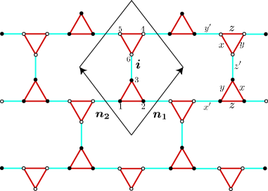
Figure 1: A piece of the triangle-honeycomb lattice which has six sites per unit cell.

III isolated-dimer limit

III.1 Mapping onto an effective spin-boson problem

Our goal is to perform a perturbative analysis of the Abelian phase around the isolated-dimer limit $J^{\prime}\gg J$. To do so, we shall use the effective spin boson mapping introduced in Ref. Schmidt et al., 2008 but, for convenience, let us first perform the following rotations :

$$\sigma_{1,{\boldsymbol{i}}}^{\alpha} \Rightarrow \widetilde{\sigma}_{1,{\boldsymbol{i}}}^{\,{\cal C}^{2}(\alpha)},\quad\sigma_{2,{\boldsymbol{i}}}^{\alpha}\Rightarrow\widetilde{\sigma}_{2,{\boldsymbol{i}}}^{\,{\cal C}(\alpha)},\quad\sigma_{3,{\boldsymbol{i}}}^{\alpha}\Rightarrow\widetilde{\sigma}_{3,{\boldsymbol{i}}}^{\alpha},$$ (3)

$$\sigma_{4,{\boldsymbol{i}}}^{\alpha} \Rightarrow \widetilde{\sigma}_{4,{\boldsymbol{i}}}^{\,{\cal C}^{2}(\alpha)},\quad\sigma_{5,{\boldsymbol{i}}}^{\alpha}\Rightarrow\widetilde{\sigma}_{5,{\boldsymbol{i}}}^{\,{\cal C}(\alpha)},\quad\sigma_{6,{\boldsymbol{i}}}^{\alpha}\Rightarrow\widetilde{\sigma}_{6,{\boldsymbol{i}}}^{\alpha},$$ (4)

where ${\cal C}$ is the cycle operator which maps $(x,y,z)$ onto $(y,z,x)$. Here, each site is encoded by a cell index ${\boldsymbol{i}}$ and a position index $k=1,\dots,6$ inside the cell as shown in Fig. 1. Hamiltonian (1) then reads

$$H = -J\sum_{{\boldsymbol{i}}}\widetilde{\sigma}_{1,{\boldsymbol{i}}}^{y}\widetilde{\sigma}_{2,{\boldsymbol{i}}}^{x}+\widetilde{\sigma}_{2,{\boldsymbol{i}}}^{y}\widetilde{\sigma}_{3,{\boldsymbol{i}}}^{x}+\widetilde{\sigma}_{3,{\boldsymbol{i}}}^{y}\widetilde{\sigma}_{1,{\boldsymbol{i}}}^{x}$$

$$-J\sum_{i}\widetilde{\sigma}_{4,{\boldsymbol{i}}}^{y}\widetilde{\sigma}_{5,{\boldsymbol{i}}}^{x}+\widetilde{\sigma}_{5,{\boldsymbol{i}}}^{y}\widetilde{\sigma}_{6,{\boldsymbol{i}}}^{x}+\widetilde{\sigma}_{6,{\boldsymbol{i}}}^{y}\widetilde{\sigma}_{4,{\boldsymbol{i}}}^{x}$$

$$-J^{\prime}\sum_{i}\widetilde{\sigma}_{1,{\boldsymbol{i}}}^{z}\widetilde{\sigma}_{4,{\boldsymbol{i}}-{\boldsymbol{n}}_{1}}^{z}+\widetilde{\sigma}_{2,{\boldsymbol{i}}}^{z}\widetilde{\sigma}_{5,{\boldsymbol{i}}-{\boldsymbol{n}}_{2}}^{z}+\widetilde{\sigma}_{3,{\boldsymbol{i}}}^{z}\widetilde{\sigma}_{6,{\boldsymbol{i}}}^{z}.$$

With this transformation, the interaction term on each dimer $(i,j)$ displayed in cyan in Fig. 1 is simply $\widetilde{\sigma_{i}}^{z}\widetilde{\sigma_{j}}^{z}$. Denoting $|\!\uparrow\rangle$ ($|\!\downarrow\rangle$) as the eigenstate of $\widetilde{\sigma}^{z}$ with eigenvalue of $+1$ ($-1$), each cyan dimer can be in four different states,

$$\begin{array}[]{lll}\{|\!\uparrow\uparrow\rangle,|\!\downarrow\downarrow\rangle\}&\mathrm{with\>\>energy}&-J^{\prime},\\ \{|\!\uparrow\downarrow\rangle,|\!\downarrow\uparrow\rangle\}&\mathrm{with\>\>energy}&+J^{\prime}.\end{array}$$ (6)

An alternative description of these four states consists in interpreting the low-energy (ferro-magnetic) states as two effective spin states without a quasiparticle and the high-energy (antiferro-magnetic) states as two effective spin states with one quasiparticle. The energy gap between these states is $\Delta=2J^{\prime}$ and corresponds to the fermionic gap evoked in Sec. II. In the following, we set once for all $J^{\prime}=1/2$ or equivalently $\Delta=1$. Among the possible mappings we choose the following : Schmidt et al. (2008)

$$|\!\uparrow\uparrow\rangle=|\!\Uparrow\!0\rangle,|\!\downarrow\downarrow\rangle=|\!\Downarrow\!0\rangle,\,|\!\uparrow\downarrow\rangle=|\!\Uparrow\!1\rangle,|\!\downarrow\uparrow\rangle=|\!\Downarrow\!1\rangle,$$ (7)

where the left (right) spin is the one of the black (white) site of the dimer, and double arrows represent the state of the effective spin.

Within this framework, each dimer is reduced to a single site with 4 degrees of freedom [one effective spin $1/2$ and a hardcore boson occupation number (0 or 1)]. Considering that each site ($\bullet$ or $\circ$, see Fig. 1) of the triangle-honeycomb lattice belongs to a cyan dimer, one then has

$$\begin{array}[]{lcl}\widetilde{\sigma}_{i,\bullet}^{x}=\tau_{i}^{x}(b^{\dagger}_{i}+b^{\phantom{\dagger}}_{i})&,&\widetilde{\sigma}_{i,\circ}^{x}=b^{\dagger}_{i}+b^{\phantom{\dagger}}_{i},\\ \widetilde{\sigma}_{i,\bullet}^{y}=\tau_{i}^{y}(b^{\dagger}_{i}+b^{\phantom{\dagger}}_{i})&,&\widetilde{\sigma}_{i,\circ}^{y}=\mathrm{i}\,\tau^{z}_{i}(b^{\dagger}_{i}-b^{\phantom{\dagger}}_{i}),\\ \widetilde{\sigma}_{i,\bullet}^{z}=\tau_{i}^{z}&,&\widetilde{\sigma}_{i,\circ}^{z}=\tau_{i}^{z}(1-2b^{\dagger}_{i}b^{\phantom{\dagger}}_{i}),\end{array}$$ (8)

where ${\tau}_{i}^{\alpha}$’s are Pauli matrices acting on the effective spin, and $b^{\dagger}_{i}$ ($b^{\phantom{\dagger}}_{i}$) is the creation (annihilation) operator of a hardcore boson at site $i$ which obeys

$$[b^{\phantom{\dagger}}_{i},b^{\dagger}_{j}]=\delta_{ij}(1-2b^{\dagger}_{i}b^{\phantom{\dagger}}_{i}).$$ (9)

Hamiltonian (III.1) then reads

$$H=-\frac{N}{2}+Q+T_{0}+T_{+2}+T_{-2},$$ (10)

where $N$ is the number of cyan dimers, $Q=\sum_{i}b_{i}^{\dagger}b_{i}$,

$$T_{0} = -J\sum_{\boldsymbol{i}}\Big{(}t_{1,{\boldsymbol{i}}}^{2,{\boldsymbol{i}}}+t_{2,{\boldsymbol{i}}}^{3,{\boldsymbol{i}}}+t_{3,{\boldsymbol{i}}}^{1,{\boldsymbol{i}}}$$

$$+t_{1,{\boldsymbol{i}}+{\boldsymbol{n}}_{1}}^{2,{\boldsymbol{i}}+{\boldsymbol{n}}_{2}}+t_{2,{\boldsymbol{i}}+{\boldsymbol{n}}_{2}}^{3,{\boldsymbol{i}}}+t_{3,{\boldsymbol{i}}}^{1,{\boldsymbol{i}}+{\boldsymbol{n}}_{1}}\Big{)}+\mathrm{H.c.},$$

$$T_{+2}=T_{-2}^{\dagger} = -J\sum_{\boldsymbol{i}}\Big{(}v_{1,{\boldsymbol{i}}}^{2,{\boldsymbol{i}}}+v_{2,{\boldsymbol{i}}}^{3,{\boldsymbol{i}}}+v_{3,{\boldsymbol{i}}}^{1,{\boldsymbol{i}}}$$

$$+v_{1,{\boldsymbol{i}}+{\boldsymbol{n}}_{1}}^{2,{\boldsymbol{i}}+{\boldsymbol{n}}_{2}}+v_{2,{\boldsymbol{i}}+{\boldsymbol{n}}_{2}}^{3,{\boldsymbol{i}}}+v_{3,{\boldsymbol{i}}}^{1,{\boldsymbol{i}}+{\boldsymbol{n}}_{1}}\Big{)},$$

with hopping operators,

$$t_{1,{\boldsymbol{i}}}^{2,{\boldsymbol{i}}} = b_{2,{\boldsymbol{i}}}^{\dagger}b_{1,{\boldsymbol{i}}}{\tau}_{1,{\boldsymbol{i}}}^{y}{\tau}_{2,{\boldsymbol{i}}}^{x},$$ (13)

$$t_{2,{\boldsymbol{i}}}^{3,{\boldsymbol{i}}} = b_{3,{\boldsymbol{i}}}^{\dagger}b_{2,{\boldsymbol{i}}}{\tau}_{2,{\boldsymbol{i}}}^{y}{\tau}_{3,{\boldsymbol{i}}}^{x},$$ (14)

$$t_{3,{\boldsymbol{i}}}^{1,{\boldsymbol{i}}} = b_{1,{\boldsymbol{i}}}^{\dagger}b_{3,{\boldsymbol{i}}}{\tau}_{3,{\boldsymbol{i}}}^{y}{\tau}_{1,{\boldsymbol{i}}}^{x},$$ (15)

$$t_{1,{\boldsymbol{i}}+{\boldsymbol{n}}_{1}}^{2,{\boldsymbol{i}}+{\boldsymbol{n}}_{2}} = -\mathrm{i}\,b_{2,{\boldsymbol{i}}+{\boldsymbol{n}}_{2}}^{\dagger}b_{1,{\boldsymbol{i}}+{\boldsymbol{n}}_{1}}{\tau}_{1,{\boldsymbol{i}}+{\boldsymbol{n}}_{1}}^{z},$$ (16)

$$t_{2,{\boldsymbol{i}}+{\boldsymbol{n}}_{2}}^{3,{\boldsymbol{i}}} = -\mathrm{i}\,b_{3,{\boldsymbol{i}}}^{\dagger}b_{2,{\boldsymbol{i}}+{\boldsymbol{n}}_{2}}{\tau}_{2,{\boldsymbol{i}}+{\boldsymbol{n}}_{2}}^{z},$$ (17)

$$t_{3,{\boldsymbol{i}}}^{1,{\boldsymbol{i}}+{\boldsymbol{n}}_{1}} = -\mathrm{i}\,b_{1,{\boldsymbol{i}}+{\boldsymbol{n}}_{1}}^{\dagger}b_{3,{\boldsymbol{i}}}{\tau}_{3,{\boldsymbol{i}}}^{z},$$ (18)

and pair-creation operators,

$$v_{1,{\boldsymbol{i}}}^{2,{\boldsymbol{i}}} = b_{2,{\boldsymbol{i}}}^{\dagger}b^{\dagger}_{1,{\boldsymbol{i}}}{\tau}_{1,{\boldsymbol{i}}}^{y}{\tau}_{2,{\boldsymbol{i}}}^{x},$$ (19)

$$v_{2,{\boldsymbol{i}}}^{3,{\boldsymbol{i}}} = b_{3,{\boldsymbol{i}}}^{\dagger}b^{\dagger}_{2,{\boldsymbol{i}}}{\tau}_{2,{\boldsymbol{i}}}^{y}{\tau}_{3,{\boldsymbol{i}}}^{x},$$ (20)

$$v_{3,{\boldsymbol{i}}}^{1,{\boldsymbol{i}}} = b_{1,{\boldsymbol{i}}}^{\dagger}b^{\dagger}_{3,{\boldsymbol{i}}}{\tau}_{3,{\boldsymbol{i}}}^{y}{\tau}_{1,{\boldsymbol{i}}}^{x},$$ (21)

$$v_{1,{\boldsymbol{i}}+{\boldsymbol{n}}_{1}}^{2,{\boldsymbol{i}}+{\boldsymbol{n}}_{2}} = \mathrm{i}\,b_{2,{\boldsymbol{i}}+{\boldsymbol{n}}_{2}}^{\dagger}b_{1,{\boldsymbol{i}}+{\boldsymbol{n}}_{1}}^{\dagger}{\tau}_{1,{\boldsymbol{i}}+{\boldsymbol{n}}_{1}}^{z},$$ (22)

$$v_{2,{\boldsymbol{i}}+{\boldsymbol{n}}_{2}}^{3,{\boldsymbol{i}}} = \mathrm{i}\,b_{3,{\boldsymbol{i}}}^{\dagger}b_{2,{\boldsymbol{i}}+{\boldsymbol{n}}_{2}}^{\dagger}{\tau}_{2,{\boldsymbol{i}}+{\boldsymbol{n}}_{2}}^{z},$$ (23)

$$v_{3,{\boldsymbol{i}}}^{1,{\boldsymbol{i}}+{\boldsymbol{n}}_{1}} = \mathrm{i}\,b_{1,{\boldsymbol{i}}+{\boldsymbol{n}}_{1}}^{\dagger}b_{3,{\boldsymbol{i}}}^{\dagger}{\tau}_{3,{\boldsymbol{i}}}^{z}.$$ (24)

Now, each site is encoded by a cell index ${\boldsymbol{i}}$ and its position inside the cell which takes three values $k=1,2,3$ as shown in Fig. 2. Within this formalism, the plaquette operators read

$$W_{{\vartriangle}}=\prod_{i\in{\vartriangle}}\tau^{z}_{i},\quad W_{{\triangledown}}=(-1)^{\sum_{i\in{\triangledown}}b^{\dagger}_{i}b^{\phantom{\dagger}}_{i}}\prod_{i\in{\triangledown}}\tau^{z}_{i},$$ (25)

for triangles and

$$W_{\hexagon}=(-1)^{b^{\dagger}_{2,{\boldsymbol{i}}}b^{\phantom{\dagger}}_{2,{\boldsymbol{i}}}+b^{\dagger}_{1,{\boldsymbol{i}}-{\boldsymbol{n}}_{2}}b^{\phantom{\dagger}}_{1,{\boldsymbol{i}}-{\boldsymbol{n}}_{2}}+b^{\dagger}_{3,{\boldsymbol{i}}-{\boldsymbol{n}}_{1}}b^{\phantom{\dagger}}_{3,{\boldsymbol{i}}-{\boldsymbol{n}}_{1}}}\prod_{{\boldsymbol{i}}\in{\hexagon}}\tau_{i}^{y},$$ (26)

for the dodecagonal plaquette (which are hexagonal in the effective lattice) located below the cell ${\boldsymbol{i}}$ (see notations in Fig. 2).

The main interest of this mapping is that the form of Hamiltonian (10) is especially adapted to the perturbative treatment developed in the Sec. III.2. Indeed, a key ingredient of our approach which is based on the continuous unitary transformations Wegner (1994) together with the particle-number conserving generator Stein (1997); Mielke (1998); Knetter and Uhrig (2000) is that the energy spectrum of the unperturbed Hamiltonian has to be equidistant.

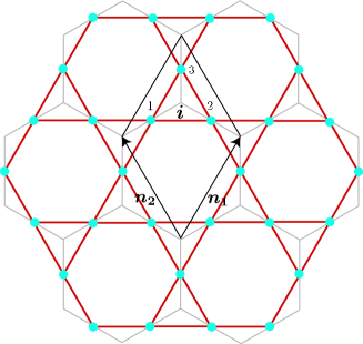
Figure 2: Effective kagome lattice obtained from the triangle-honeycomb lattice by replacing each dimer linking triangles by a site. We displayed in gray the “dual” honeycomb lattice on which the toric code is defined (see text).

III.2 Perturbative analysis of the low-energy sector

In this section, we used exactly the same method as those described in Refs. Schmidt et al., 2008 and Vidal et al., for the Kitaev honeycomb model. Therefore, we skipped all technical details and only give here the results of our calculations.

First, let us note that, in the triangle-honeycomb lattice, one has

$$N_{\mathrm{s}}=3N_{\mathrm{t}}=6N_{\mathrm{d}}=2N,$$ (27)

where $N$ is the number of cyan dimers and $\mathrm{s}$, $\mathrm{t}$, and $\mathrm{d}$ stand, respectively for sites, triangles (so $N_{\mathrm{t}}=N_{\vartriangle}+N_{\triangledown}$), and dodecagons (or effective hexagons, so $N_{\mathrm{d}}=N_{\hexagon}$). There are thus as many conserved $\mathbb{Z}_{2}$ plaquette operators $N_{\mathrm{t}}+N_{\mathrm{d}}$ as the number $N$ of effective spin 1/2. This implies that in the low-energy subspace with no hardcore boson, the effective Hamiltonian can, in the isolated-dimer limit $J^{\prime}\gg J$, be written only in terms of the plaquette operators, and is thus readily solved. The general form of this effective Hamiltonian reads

$$H_{\mathrm{eff}}^{(0)}=E_{0}-\sum_{p_{1},\ldots,p_{n}}C_{p_{1},\ldots,p_{n}}W_{p_{1}}W_{p_{2}}\ldots W_{p_{n}},$$ (28)

where ${p_{1},\ldots,p_{n}}$ denotes a set of $n$ plaquettes.

We performed this perturbative expansion of the effective Hamiltonian up to order $8$ which is the lowest order involving multi-plaquette interactions. At this order, the constant term is given by

$$\frac{E_{0}}{N}=-\frac{1}{2}-J^{2}-\frac{1}{4}J^{4}-\frac{1}{8}J^{6}+\frac{15}{64}J^{8}.$$ (29)

The first nontrivial contribution arises at order 6 where only hexagonal-plaquette operators are involved. At order 8, this latter term is renormalized and triangular-plaquette operators come into play. More precisely, one has

$$H_{\mathrm{eff}}^{(0)}=E_{0}-C_{h}\sum_{h}W_{h}-C_{h,t_{1},t_{2}}\sum_{h,t_{1},t_{2}}W_{h}W_{t_{1}}W_{t_{2}},$$ (30)

where the first sum is performed over all hexagonal plaquettes $h$ (i.e. ${\hexagon}$) and the second one over triplet plaquettes made of one hexagon $h$ and two triangles $t_{1}$ and $t_{2}$ (of any kind $\vartriangle$ or $\triangledown$) adjacent to this hexagon. At order 8, the coefficients are given by

$$C_{h}=\frac{63}{8}J^{6}-\frac{297}{8}J^{8},\quad C_{h,t_{1},t_{2}}=\frac{33}{16}J^{8}.$$ (31)

Thus, at order 6, the spectrum does not depend on the fluxes inside the triangles and this degeneracy is only partially lifted at order 8. Note that the signs of $C_{h}$ and $C_{h,t_{1},t_{2}}$ confirm, in this limit, that (one of) the ground state lies in the vortex-free sector ($w_{p}=+1$ for all plaquettes) as conjectured in Ref. Yao and Kivelson, 2007. In addition, we emphasize that triangular-plaquette operators appear by pairs which are reminiscent from the time-reversal symmetry that the effective Hamiltonian must satisfy (see Sec. II).

It is interesting to interpret this result in terms of plaquettes and vertex operators. Therefore, one may view the effective kagome lattice as a honeycomb lattice where each site lies in the middle of the triangles as shown in Fig. 2. Within this picture, the plaquette operators $W_{\hexagon}$ are interpreted as flux (magnetic) operators, whereas $W_{{\vartriangle},{\triangledown}}$ appear as vertex (electric) operators. In this gauge theory language used in the toric-code model Kitaev (2003), our results show that, at lowest order, there is no contribution of the vertex operators. Thus, the triangle-honeycomb lattice, in this isolated-dimer limit does not map onto a standard toric-code-like problem. However, the eigenstates of the effective Hamiltonian are those of the toric code on the hexagonal lattice and, as such, display anyonic statistics. To be more precise, one must distinguish between electric and magnetic excitations which are localized on triangles and hexagons (in the kagome lattice), respectively. These two kinds of excitations have mutual semionic statistics Kitaev (2003); Yao and Kivelson (2007) but they individually behave as bosons. Finally, let us remark that the gaps of magnetic excitations (order of magnitude $J^{6}$) and of electric excitations (order of magnitude $J^{8}$) are even smaller than the gap in the Kitaev honeycomb model (order of magnitude $J^{4}$). This would make an experimental detection of anyons in the triangle-honeycomb model even more problematic than in the honeycomb model Dusuel et al. (2008).

III.3 Correlation functions in the low-energy sector

As in the Kitaev honeycomb model, any correlator involving an odd number of spin operators vanishes although the eigenstates break the time-reversal symmetry. Indeed, as discussed by Yao and Kivelson Yao and Kivelson (2007), every eigenstate is, at least, two-fold degenerate since one can flip every triangular plaquette without changing the energy but this operation is global. Consequently, as in the honeycomb model Baskaran et al. (2007); Chen and Nussinov (2008), the only nonvanishing correlators are products of $\sigma^{\alpha}_{i}\sigma^{\alpha}_{j}$ on an $\alpha$ dimers. Here, we focus on the simplest case involving only one such object, i.e., $C^{\alpha\alpha}_{i,j}=\langle\sigma^{\alpha}_{i}\sigma^{\alpha}_{j}\rangle$.

In the triangle-honeycomb model, one has, a priori, nine different functions to consider since the unit cell contains nine different dimers. However, with the choice of the couplings we made, one only has two different functions to distinguish : those on “weak” bonds ($x,y,z$ links with interaction $J$) and those on “strong” bonds ($x^{\prime},y^{\prime},z^{\prime}$ links with interaction $J^{\prime}$). As for the low-energy spectrum, one expects a plaquette-operator expansion as in Eq. (28). We performed the calculation of these two correlation functions up to order 6 and obtained

$$C^{\mathrm{strong}}_{i,j}=1-2J^{2}-\frac{3}{2}J^{4}-\frac{5}{4}J^{6}-\frac{105}{8}J^{6}\left(W_{p_{1}}+W_{p_{2}}\right),$$ (32)

where $p_{1}$ and $p_{2}$ are the two dodecagonal plaquettes shared by the considered strong bond $(i,j)$. Similarly, since we set $J_{x}=J_{y}$, we found for a weak bond $(i,j)$

$$C^{\mathrm{weak}}_{i,j}=J+\frac{1}{2}J^{3}+\frac{3}{8}J^{5}+\frac{63}{8}J^{5}W_{p},$$ (33)

where $p$ is the dodecagonal plaquette adjacent to the considered bond.

As can be seen from Eqs. (32) and (33), the presence of a vortex is detected at orders 6 and 5, respectively. This difference stems from the fact that one analyzes the isolated-dimer limit for which, at lowest order, $C^{\mathrm{strong}}_{i,j}=1$ whereas $C^{\mathrm{weak}}_{i,j}=0$.

III.4 Checks from Majorana fermions

To check our results we computed exactly the ground-state energy in the vortex-free (full) sector for which $w_{p}=+1$ (-1) for all $p$ using Majorana fermions as described by Kitaev for the honeycomb model Kitaev (2006). Following, the procedure described in Ref. Vidal et al., , we performed a perturbative expansion of the exact solutions order by order. Denoting $e_{0}^{\nu}$ the ground-state energy per cyan dimer for a vortex filling factor $\nu=\frac{\rm Number\>\>of\>\>vortex}{\rm Number\>\>of\>\>plaquette}$ one gets

$$e_{0}^{\nu=0} = -J^{\prime}-\frac{J^{2}}{2J^{\prime}}-\frac{J^{4}}{32J^{\prime 3}}-\frac{11J^{6}}{128J^{\prime 5}}+\frac{147J^{8}}{8192J^{\prime 7}},\quad$$ (34)

$$e_{0}^{\nu=1} = -J^{\prime}-\frac{J^{2}}{2J^{\prime}}-\frac{J^{4}}{32J^{\prime 3}}+\frac{5J^{6}}{64J^{\prime 5}}-\frac{117J^{8}}{8192J^{\prime 7}}.$$ (35)

Keeping in mind that the number of hexagons is $N/3$ and that for each hexagon $\mathrm{h}$, there are 15 triplets $\mathrm{h,t_{1},t_{2}}$, these results are straightforwardly recovered using Eqs. (29)-(31).

One can also check the expression of the correlation functions in these vortex configurations. Indeed, the Hellmann-Feynman theorem states that

$$\frac{\partial e_{0}^{\nu}}{\partial J^{\prime}} = -\frac{1}{N}\sum_{(i,j)}C^{\mathrm{strong}}_{i,j}=-C^{\mathrm{strong}}_{i,j},$$ (36)

$$\frac{\partial e_{0}^{\nu}}{\partial J} = -\frac{1}{N}\sum_{(i,j)}C^{\mathrm{weak}}_{i,j}=-2\ C^{\mathrm{weak}}_{i,j},$$ (37)

where the sum in Eq. (36) [Eq. (37)] is performed over all strong bonds (weak bonds) in the initial lattice. The last equalities stem from the fact that for $\nu=0,1$ every plaquette has the same contribution which would not be true for other vortex configurations. Using Eqs. (34) and (35) and the above relations, one can easily check the validity of Eqs. (32) and (33).

IV isolated-triangle limit

IV.1 Mapping to a spin-boson plaquette problem

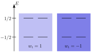
Figure 3: Spectrum of an isolated triangle with $J=\frac{1}{2\sqrt{3}}$. The eigenstates have quantum number $w_{\mathrm{t}}=1$ (left) or $w_{\mathrm{t}}=-1$ (right).

Let us now turn to the isolated-triangle limit $J\gg J^{\prime}$. These triangles live on the sites of an effective hexagonal lattice. For convenience, we use rotated form (III.1) that was already used in the isolated-dimer limit. The spectrum of the Hamiltonian of an isolated triangle is made of two sets of fourfold-degenerate levels. In each of these sets, two levels have eigenvalue $w_{\mathrm{t}}=1$ and the other two $w_{\mathrm{t}}=-1$. Setting $J=\frac{1}{2\sqrt{3}}$, the eigenenergies are $\pm 1/2$. This information is gathered in Fig. 3.

As in the isolated-dimer limit, we interpret low (high) energy states of an isolated triangle as containing zero (one) hardcore boson. This hardcore boson degree of freedom, which we again denote as $b$, together with the $\mathbb{Z}_{2}$ quantum number $w_{\mathrm{t}}$ span a four-dimensional Hilbert space. It is then natural to introduce an effective spin 1/2 to span the full eight-dimensional Hilbert space of a triangle. We again denote this effective spin as $\tau$ (though it is not the same as in the other perturbative limit, and the same remark holds for $b$). The way this effective spin is introduced is partly dictated by the operators involved in the adjacent dodecagonal-plaquette operators. For the triangle $(1,2,3)$ of Fig. 1 (and dropping the ${\boldsymbol{i}}$ index), the mapping reads

$$\tau^{x}=W_{\mathrm{t}}{\widetilde{\sigma}}_{2}^{x}{\widetilde{\sigma}}_{3}^{y},\quad\tau^{y}=W_{\mathrm{t}}{\widetilde{\sigma}}_{3}^{x}{\widetilde{\sigma}}_{1}^{y},\quad\tau^{z}=-W_{\mathrm{t}}{\widetilde{\sigma}}_{1}^{x}{\widetilde{\sigma}}_{2}^{y}.$$ (38)

It is straightforward to check that the above $\tau^{\alpha}$ operators satisfy the usual Pauli matrices algebra. The product ${\widetilde{\sigma}}_{2}^{x}{\widetilde{\sigma}}_{3}^{y}$ appearing in $\tau^{x}$, for example, is the same as the one that appears in the dodecagonal-plaquette operator having the bond $(2,3)$ in common with the triangle. It is interesting to note that one has to use the operator $W_{\mathrm{t}}={\widetilde{\sigma}}_{1}^{z}{\widetilde{\sigma}}_{2}^{z}{\widetilde{\sigma}}_{3}^{z}$ to fulfill the SU(2) algebra. The same mapping is used for the other triangles, with $1,2$, and $3$ simply replaced by $4,5$, and $6$ (see Fig. 1 for notations).

Since the terms proportional to $J$ in Eq. (III.1) now read $-N_{\mathrm{t}}/2+Q$, with $Q=\sum_{\boldsymbol{i}}b^{\dagger}_{\boldsymbol{i}}b^{\phantom{\dagger}}_{\boldsymbol{i}}$ where the sum runs over the sites ${\boldsymbol{i}}$ of the effective hexagonal lattice (formed by triangles), the last task in rewriting Hamiltonian (III.1) is to find the new form of the terms proportional to $J^{\prime}$. A simple but lengthy calculation yields

$$H=-N_{\mathrm{t}}/2+Q-\frac{J^{\prime}}{3}\sum_{\alpha=x,y,z}\sum_{\alpha-\mathrm{links}}\mathcal{O}_{\boldsymbol{i}}^{\alpha}\mathcal{O}_{\boldsymbol{j}}^{\alpha},$$ (39)

where $\alpha$ indicates a link of type $x$, $y$, or $z$ on the honeycomb or equivalently brickwall lattice, with the conventions of Kitaev Kitaev (2006), as shown in Fig. 4. Furthermore ${\boldsymbol{i}}$ and ${\boldsymbol{j}}$ are the sites of the effective brickwall lattice on link $\alpha$, and the operators $\mathcal{O}_{\boldsymbol{i}}^{\alpha}$ reads ($W_{\mathrm{t},{\boldsymbol{i}}}$ denotes the triangular-plaquette operator which is now associated to site ${\boldsymbol{i}}$)

$$\mathcal{O}_{\boldsymbol{i}}^{\alpha}=\tau_{\boldsymbol{i}}^{\alpha}\Bigg{\{}(-1)^{b^{\dagger}_{\boldsymbol{i}}b^{\phantom{\dagger}}_{\boldsymbol{i}}}-\sqrt{2}W_{\mathrm{t},{\boldsymbol{i}}}\left[\mathrm{e}^{\frac{2\mathrm{i}\pi}{3}p^{\alpha}W_{\mathrm{t},{\boldsymbol{i}}}}\,b^{\dagger}_{\boldsymbol{i}}+\mathrm{H.c.}\right]\Bigg{\}},$$ (40)

where $p^{x}=1,p^{y}=-1$, and $p^{z}=0$.

IV.2 Perturbation analysis of the low-energy sector

From the above expressions, it is clear that the Hamiltonian can now be written

$$H=-\frac{N_{\mathrm{t}}}{2}+Q+T_{0}+T_{+1}+T_{-1}+T_{+2}+T_{-2},$$ (41)

where the operators $T_{n}$ change the number of bosons by $n$ and are proportional to $J^{\prime}$. With our notations, they read

$$T_{n}=-\frac{J^{\prime}}{3}\sum_{\alpha=x,y,z}\sum_{\alpha-\mathrm{links}}\tau_{\boldsymbol{i}}^{\alpha}\tau_{\boldsymbol{j}}^{\alpha}\,\mathcal{T}^{\alpha}_{n,{\boldsymbol{i}},{\boldsymbol{j}}},$$ (42)

with

$$\mathcal{T}^{\alpha}_{0,{\boldsymbol{i}},{\boldsymbol{j}}} = (-1)^{b^{\dagger}_{\boldsymbol{i}}b^{\phantom{\dagger}}_{\boldsymbol{i}}+b^{\dagger}_{\boldsymbol{j}}b^{\phantom{\dagger}}_{\boldsymbol{j}}}$$

$$+2\,W_{\mathrm{t},{\boldsymbol{i}}}W_{\mathrm{t},{\boldsymbol{j}}}\left[\mathrm{e}^{\frac{2\mathrm{i}\pi}{3}p^{\alpha}(W_{\mathrm{t},{\boldsymbol{i}}}-W_{\mathrm{t},{\boldsymbol{j}}})}\,b^{\dagger}_{\boldsymbol{i}}b^{\phantom{\dagger}}_{\boldsymbol{j}}+\mathrm{H.c.}\right],$$

$$\mathcal{T}^{\alpha}_{1,{\boldsymbol{i}},{\boldsymbol{j}}} = -\sqrt{2}\Big{[}W_{\mathrm{t},{\boldsymbol{i}}}\,\mathrm{e}^{\frac{2\mathrm{i}\pi}{3}p^{\alpha}W_{\mathrm{t},{\boldsymbol{i}}}}\,b^{\dagger}_{\boldsymbol{i}}\,(-1)^{b^{\dagger}_{\boldsymbol{j}}b^{\phantom{\dagger}}_{\boldsymbol{j}}}+({\boldsymbol{i}}\leftrightarrow{\boldsymbol{j}})\Big{]}$$

$$\mathcal{T}^{\alpha}_{2,{\boldsymbol{i}},{\boldsymbol{j}}} = 2\,W_{\mathrm{t},{\boldsymbol{i}}}W_{\mathrm{t},{\boldsymbol{j}}}\,\mathrm{e}^{\frac{2\mathrm{i}\pi}{3}p^{\alpha}(W_{\mathrm{t},{\boldsymbol{i}}}+W_{\mathrm{t},{\boldsymbol{j}}})}\,b^{\dagger}_{\boldsymbol{i}}b^{\dagger}_{\boldsymbol{j}},$$ (46)

$$T_{-1}=T_{1}^{\dagger},\quad\mathrm{and}\quad T_{-2}=T_{2}^{\dagger}.$$

Figure 4: A piece of the effective brickwall lattice spanned by triangles, together with the notations for $x$, $y$, and $z$ links (left). Filled (empty) dots represent the triangles made of filled (empty) dots in Fig. 1. On the right, we have represented one of the second-order three-spin terms that appear in Eq. (48).

As in the isolated-dimer limit (where $T_{\pm 1}$ terms are absent), with a suitable unitary transformation, such a Hamiltonian can be recasted in a unitary equivalent effective form $H_{\mathrm{eff}}$ which conserves the number of bosons, i.e., that commutes with $Q$. We refer the reader to Ref. Knetter and Uhrig, 2000 (especially Appendix B), from which it follows that at order 2,

$$H_{\mathrm{eff}}=-\frac{N_{\mathrm{t}}}{2}+Q+T_{0}+\left[T_{+1},T_{-1}\right]+\frac{1}{2}\left[T_{+2},T_{-2}\right].$$ (47)

A tedious calculation then shows that in the low-energy subspace with no boson, the effective Hamiltonian (still at order 2) has the form

$$H_{\mathrm{eff}}^{(0)} = -\frac{N_{\mathrm{t}}}{2}\left(1+2{J^{\prime}}^{2}\right)-\frac{J^{\prime}}{3}\sum_{\alpha}\sum_{\alpha-\mathrm{links}}\tau_{\boldsymbol{i}}^{\alpha}\tau_{\boldsymbol{j}}^{\alpha}$$ (48)

$$+\frac{2\sqrt{3}{J^{\prime}}^{2}}{9}{\sum_{{\boldsymbol{i}},{\boldsymbol{j}},{\boldsymbol{k}}}}^{\prime}W_{\mathrm{t},{\boldsymbol{j}}}\,\tau_{\boldsymbol{i}}^{\alpha}\tau_{\boldsymbol{j}}^{\beta}\tau_{\boldsymbol{k}}^{\gamma}.$$

The low-energy effective Hamiltonian at order 1 is nothing but that of the Kitaev honeycomb model at the isotropic point, though one should remember that site ${\boldsymbol{i}}$ now also has the $\mathbb{Z}_{2}$ supplementary degree of freedom $W_{\mathrm{t},{\boldsymbol{i}}}$. In Eq. (48), the last (primed) sum is to be taken over all possible combinations of three sites ${\boldsymbol{i}}$, ${\boldsymbol{j}}$, and ${\boldsymbol{k}}$ such that ${\boldsymbol{i}}$ and ${\boldsymbol{k}}$ are nearest neighbors of ${\boldsymbol{j}}$, and the spin “directions” $\alpha$, $\beta$, and $\gamma$ are such that $({\boldsymbol{i}},{\boldsymbol{j}})$ is an $\alpha$ link, $({\boldsymbol{j}},{\boldsymbol{k}})$ is a $\gamma$ link, and $\beta$ is the outgoing direction at site ${\boldsymbol{j}}$ of the path $({\boldsymbol{i}},{\boldsymbol{j}},{\boldsymbol{k}})$ (note that $\alpha$, $\beta$ and $\gamma$ are all distinct). For clarity, one such term is illustrated in Fig. 4 (right). These terms, apart from the plaquette operator $W_{\mathrm{t},{\boldsymbol{j}}}$, are exactly the ones that arise when switching a magnetic field on, in the gapless phase of the Kitaev honeycomb model. They open a gap and give proper non-Abelian anyonic statistics to the vortices, as detailed in Ref. Kitaev, 2006. Actually, one does not know how to diagonalize analytically $H_{\mathrm{eff}}^{(0)}$ for arbitrary vortex configurations even at order 1 Kitaev (2006) and, in particular, how to obtain the ground state of each sector. Therefore, contrary to the isolated-dimer limit, one cannot compute the correlation functions in this limit.

Let us remark that the plaquette operators on an elementary brick (or hexagon) $h$, namely $W_{h}=\prod_{{\boldsymbol{i}}\in h}\tau_{\boldsymbol{i}}^{\mathrm{out}({\boldsymbol{i}})}$ are the product of the plaquette operators of the corresponding dodecagon on the original lattice and of its adjacent triangles, as follows from Eq. (38). From Eq. (48) and the previous remarks, it follows that the vortex-free sector contains non-Abelian anyons, which is consistent with the findings of Ref. Yao and Kivelson, 2007. One can also use Kitaev’s result (see Sec. 8 of Ref. Kitaev, 2006) to obtain the gap in this sector,

$$\Delta=6\sqrt{3}\times\frac{2\sqrt{3}{J^{\prime}}^{2}}{9}=4{J^{\prime}}^{2},$$ (49)

in units where $J=\frac{1}{2\sqrt{3}}$, and thus also $\Delta=\frac{2\sqrt{3}{J^{\prime}}^{2}}{3J}$ if $J$ is chosen freely. This value of the gap is consistent with the numerical results obtained by Yao and KivelsonYao and Kivelson (2007), and we also checked it using an expansion of the exact result from Majorana fermionization. We also checked that the ground-state energies in the vortex-free sector obtained, thanks to a Majorana fermionization of Hamiltonian (48) or directly of initial Hamiltonian (1), match at order 2.

Finally, let us mention that at order 1, the ground states of Eq. (48) are such that $W_{h}=1$ for all $h$. There are many such states. The vortex-free state is such a state, but any configuration where the six triangles surrounding one dodecagon are flipped to $W_{\mathrm{t}}=-1$ is also such a state, since every dodecagon is then surrounded by an even number of flipped triangles. From form (48) at order 2, we do not know how to prove that the ground state is the vortex-free state (we do not even know if this is true or if one has to go to higher orders in perturbation to prove it). We leave this as an open question.

V Conclusion

In this work, we have studied perturbatively the Kitaev model on the triangle-honeycomb model. This has allowed us to show that in the isolated-dimer limit, the model has low-energy Abelian anyonic excitations, whereas in the isolated-triangle limit, the anyons become non-Abelian. This picture is consistent with the values of the Chern number in each of these phases Yao and Kivelson (2007). In the isolated-dimer limit, we have furthermore computed the low-energy spectrum, as well as the spin-spin correlation functions, which both display a plaquette expansion. We emphasize that such a computation is not an easy task within the Majorana or Jordan-Wigner formalism, which are only well suited to study analytically configurations of vortices which display translational invariance.