Abstract

We discuss generic properties of rotating nonlinear wave solutions, the so called azimuthons, in nonlocal media. Variational methods allow us to derive approximative values for the rotating frequency, which is shown to depend crucially on the nonlocal response function. Further on, we link families of azimuthons to internal modes of classical non-rotating stationary solutions, namely vortex and multipole solitons. This offers an exhaustive method to identify azimuthons in a given nonlocal medium.

OCIS codes: 190.0190, 190.4420

1 Introduction

Spatial trapping of light in nonlinear media is a result of a balance between diffraction and the self-induced nonlinear index change [1, 2]. As the rate of diffraction is determined by the spatial scale of the light beam independently of its dimensionality the stability properties of the self-trapped beams critically depend on the particular model of the nonlinear response of the medium. Commonly encountered in the context of nonlinear optics the, so called, Kerr nonlinearity with nonlinear index change being proportional to light intensity leads to stable spatial solitons only in one transverse dimension. For two dimensional beams the same model does not permit stable beam localization. Instead, it predicts either eventual diffraction or catastrophic collapse for input power below or above a certain threshold value, respectively [3]. Hence, in order to ensure the existence of stable self-localized beams in two dimensions different nonlinear response is necessary. It is known that the saturation of nonlinearity at high intensities is sufficient to prevent collapse and provide stabilization of finite beams (see [4] and references therein). However, saturable nonlinearity cannot stabilize complex localized structures such as vortex beams which are prone to azimuthal instability [5]. It has been shown recently that stabilization of localized waves is greatly enhanced in the nonlocal nonlinear media. In such media nonlinear response in a particular spatial location is typically determined by the wave intensity in a certain neighborhood of this location. Nonlocality often results from certain transport processes such as atomic diffusion [6], ballistic transport of hot atoms or molecules [7] or heat transfer [8, 9]. It can be also a signature of a long-range interparticle interaction such as in nematic liquid crystals [10, 11, 12]. Spatially nonlocal response is also naturally present in atomic condensates where it describes a noncontact bosonic interaction [13, 14, 15]. Extensive studies of beam propagation in nonlocal nonlinear media revealed a range of interesting features. In particular, it has been shown that nonlocality may affect modulational instability of plane waves [16] and prevent catastrophic collapse of finite beams [17, 18] as well as stabilize complex one- and two-dimensional beams including vortices [19, 20, 21, 22, 23, 24]. Recently, it has been shown that nonlocal media can also support stable propagation of the rotating solitons, the so called azimuthons [25]. Azimuthons have been originally proposed in the context of local nonlinear media [26]. They are azimuthally modulated beams with nontrivial phase structures exhibiting steady angular rotation upon propagation. They can be considered as azimuthally perturbed optical vortices, i.e. beams with singular phase structure [27]. Recent theoretical studies demonstrated both, stable and unstable evolution of azimuthons [28, 29]. In the former case it has been shown that in a highly nonlocal regimes azimuthons undergo structural transformation resulting from the energetic coexistence of solitons of different symmetries. Numerical and analytical studies revealed that the angular velocity of azimuthons is governed by two contributions. The linear component, determined solely by the spatial structure of the beam (akin to rotation of complex wave structures resulting from beating of their constituent modes [30]) as well as the nonlinear which is brought about by the nonlinearity [29].

In this work we investigate in details rotating nonlocal solitons. We consider various nonlocal models and show how they determine dynamical properties of azimuthons. In particular, we will show that both, rotational frequency and intensity profile of the azimuthons can be uniquely determined by analyzing Eigenmodes of the linearized version of the corresponding nonlocal problem. The paper is organized as follows: In Sec. 2 we introduce the model equations, the general ansatz for rotating solitons (azimuthons) and an exact expression for their rotation frequency. In Sec. 3, we derive an approximative, variational formula for the rotation frequency of the dipole azimuthons. In Sec. 4 we confront our semi-analytical results with exact numerical solutions of the ensuing nonlinear equations. One of our main findings is that azimuthons emerge from internal modes of stationary nonlinear soliton solutions like vortex or dipole, which is detailed in Sec. 5.

2 Rotating Solutions

We consider physical systems governed by the two-dimensional nonlocal nonlinear Schrödinger equation

$$i\frac{\partial}{\partial z}\psi+\Delta_{\perp}\psi+\theta\psi=0.$$ (1)

where $\theta$ represents the spatially nonlocal nonlinear response of the medium. Its form depends on the details of a particular physical system.

In the so called Gaussian model of nonlocality, $\theta$ is given as

$$\theta=\frac{1}{2\pi}\iint\mathrm{e}^{-\frac{|\vec{r}-\vec{r}^{\prime}|^{2}}{2}}\left|\psi(\vec{r}^{\prime},z)\right|^{2}d^{2}\vec{r}^{\prime},$$ (2)

where $\vec{r}=x\vec{e}_{x}+y\vec{e}_{y}$ denotes the transverse coordinates.

If $\theta$ is governed by the following diffusion-type equation

$$\theta-\Delta_{\perp}\theta=|\psi|^{2},$$ (3)

solving formally Eq. (3) in the Fourier space yields

$$\theta=\frac{1}{2\pi}\iint\mathfrak{K}_{0}(|\vec{r}-\vec{r}^{\prime}|)\left|\psi(\vec{r}^{\prime},z)\right|^{2}d^{2}\vec{r}^{\prime},$$ (4)

where $\mathfrak{K}_{0}$ is the modified Bessel function of the second kind.

In the following, we will assume that the nonlinear response $\theta$ can be expressed in terms of the nonlocal response function $R(r)$

$$\theta=\iint R(|\vec{r}-\vec{r}^{\prime}|)\left|\psi(\vec{r}^{\prime},z)\right|^{2}d^{2}\vec{r}^{\prime},$$ (5)

and Eqs. (2) and (4) will serve as prominent examples.

Azimuthons are a straightforward generalization of the usual ansatz for stationary solutions (solitons) [26]. They represent spatially rotating structures and hence involve an additional parameter, the angular frequency $\Omega$

$$\psi(r,\phi,z)=U(r,\phi-\Omega z)\mathrm{e}^{i\lambda z},$$ (6)

where $U$ is the complex amplitude function and $\lambda$ the propagation constant. For $\Omega=0$, azimuthons become ordinary (nonrotating) solitons. The most simple family of azimuthons is the one connecting the dipole soliton with the single charged vortex soliton [25]. A single charged vortex consists of two equal-amplitude dipole-shaped structures representing real and imaginary part of $U$. If these two components differ in amplitudes the resulting structure forms a ”rotating dipole” azimuthon. If one of the components is zero we deal with the (nonrotating) dipole soliton. In the following we will denote the ratio of these two amplitudes by $\alpha$, which also determines the angular modulation depth of the resulting ring-like structure by “$1-\alpha$” .

After inserting the ansatz (6) into Eqs. (1) and (5), multiplying with $U^{*}$ and $\partial_{\phi}U^{*}$ resp., and integrating over the transverse coordinates we end up with

$$-\lambda M+\Omega L_{z}+I+N =0$$ (7a)

$$-\lambda L_{z}+\Omega M^{\prime}+I^{\prime}+N^{\prime} =0.$$ (7b)

This system relates the propagation constant $$\lambda \Omega$$ and the rotation frequency of the azimuthons to integrals over their stationary amplitude profiles, namely

$$M =\iint\left|U(\vec{r})\right|^{2}d^{2}\vec{r}$$ (7c)

$$L_{z} =-i\iint U^{*}(\vec{r})\frac{\partial}{\partial\phi}U(\vec{r})d^{2}\vec{r}$$ (7d)

$$I =\iint U^{*}(\vec{r})\Delta_{\perp}U(\vec{r})d^{2}\vec{r}$$ (7e)

$$N =\iiiint R(|\vec{r}-\vec{r}^{\prime}|)\left|U(\vec{r}^{\prime})\right|^{2}\left|U(\vec{r})\right|^{2}d^{2}\vec{r}^{\prime}d^{2}\vec{r}$$ (7f)

$$M^{\prime} =\iint\left|\frac{\partial}{\partial\phi}U(\vec{r})\right|^{2}d^{2}\vec{r}$$ (7g)

$$I^{\prime} =i\iint\left[\frac{\partial}{\partial\phi}U^{*}(\vec{r})\right]\Delta_{\perp}U(\vec{r})d^{2}\vec{r}$$ (7h)

$$N^{\prime} =i\iiiint R(|\vec{r}-\vec{r}^{\prime}|)\left|U(\vec{r}^{\prime})\right|^{2}\left[\frac{\partial}{\partial\phi}U^{*}(\vec{r})\right]U(\vec{r})d^{2}\vec{r}^{\prime}d^{2}\vec{r}.$$ (7i)

The first two quantities have straightforward physical meanings, namely ”mass” ($M$) and ”angular momentum” ($L_{z}$). We can formally solve for the rotation frequency and obtain (for an alternative derivation see [31])

$$\Omega=\frac{M\left(I^{\prime}+N^{\prime}\right)-L_{z}\left(I+N\right)}{L_{z}^{2}-MM^{\prime}}.$$ (8)

Note that this expression is undetermined for a vortex beam (see discussion below).

While the above formula looks simple its use requires detailed knowledge of the actual solution which can only be obtained numerically. However, it turns out that it is still possible to analyze main features of rotating solitons using simple approximate approach. To this end let us consider the ”rotating dipole”. Obviously, we have $\Omega=0$ for $\alpha=0$ (dipole soliton). On the other hand, for $\alpha=1$ [vortex soliton $V(r)\exp(i\phi+i\lambda_{0}z$)], we can assume any value for $\Omega$ by just shifting the propagation constant $\lambda=\lambda_{0}+\Omega$ accordingly ($\lambda_{0}$ accounts for the propagation constant in the non-rotating laboratory frame). However, with respect to the azimuthon in the limit $\alpha\rightarrow 1$, the value of $\Omega$ is fixed. In what follows, we denote this value by $\Omega|_{\alpha=1}$.

3 Rotation Frequency - Approximate Analysis

In a first attempt, let us assume we know the radial shape of the vortex soliton $V(r)$. Then, a straight forward approximative ansatz for the dipole azimuthons is [28, 29]

$$U(r,\phi-\Omega z)=AV(r)\left[\cos(\phi-\Omega z)+i\alpha\sin(\phi-\Omega z)\right],$$ (9)

where $A$ is an amplitude factor. The family of the ”rotating dipole” azimuthons has two parameters, e.g. $\lambda$ and $\Omega$. Here, for technical reasons, we prefer to use the mass $M$ and the amplitude ratio $\alpha$. We take the radial shape of the vortex for a given mass $M_{0}$ and fix the amplitude factor $A$ in ansatz (9) to $A=\sqrt{2/(\alpha^{2}+1)}$. With this choice the mass of the azimuthon equals $M_{0}$ for all values of $\alpha$. Then, we can compute all integrals in Eqs. (7) as functions of $\alpha$: $M=M_{0}$, $L_{z}=2\alpha M_{0}/(\alpha^{2}+1)$, $I=I_{0}$, $N=[4(1+\alpha^{4})N_{\mathrm{cc}}+8\alpha^{2}N_{\mathrm{cs}}]/(\alpha^{2}+1)^{2}$, $M^{\prime}=M_{0}$, $I^{\prime}=2\alpha I_{0}/(\alpha^{2}+1)$, and $N^{\prime}=4\alpha(N_{\mathrm{cc}}+N_{\mathrm{cs}})/(\alpha^{2}+1)$. The index ”$0$” indicates the value of the respective integral for the vortex (i.e., for $\alpha=1$), and

$$N_{\mathrm{cc}} =\iiiint R(|\vec{r}-\vec{r}^{\prime}|)V^{2}(r^{\prime})\cos^{2}(\phi^{\prime})V^{2}(r)\cos^{2}(\phi)d^{2}\vec{r}^{\prime}d^{2}\vec{r}$$ (10a)

$$N_{\mathrm{cs}} =\iiiint R(|\vec{r}-\vec{r}^{\prime}|)V^{2}(r^{\prime})\cos^{2}(\phi^{\prime})V^{2}(r)\sin^{2}(\phi)d^{2}\vec{r}^{\prime}d^{2}\vec{r}.$$ (10b)

Finally, we obtain the following simple expression for the rotation frequency from Eq. (8),

$$\Omega=\frac{2\alpha}{\alpha^{2}+1}\frac{2\left(N_{\mathrm{cc}}-N_{\mathrm{cs}}\right)}{M_{0}}.$$ (11)

Let us have a closer look at this approximation. First of all, we have $N_{\mathrm{cc}}\geq N_{\mathrm{cs}}$ if we assume $R(r)$ to be monotonically decreasing in $r>0$. This immediately implies that the sense of the amplitude rotation is opposite to that of the phase rotation. In general, we need to know the actual shape of the vortex soliton to compute Eq. (11). One possibility would be to use exact numerical solutions of the vortex shape $V$, a time consuming task because $V$ depends in nontrivial way on $\lambda_{0}$. Moreover, Eq. (11) is only an approximation to $\Omega$ and should not require the exact shapes. Luckily, it is possible to compute quite good approximative vortex solitons using the so called variational approach [32]. We employ the following ansatz $V=Ar\exp(-r^{2}/2\sigma^{2})$, $U=V\exp(i\phi)$, $\psi=U\exp(i\lambda_{0}z)$ and look for critical points of the Lagrangian $\mathcal{L}=-\lambda_{0}M+I+N/2$ with respect to the variables $A$ and $\sigma$. In the following, we give results for our two exemplary nonlocal nonlinearities.

For the Gaussian response, Eq. (2), all integrals appearing in the variational approach can be evaluated analytically. Hence, we find the width $\sigma$ of our approximate solution as

$$\lambda_{0}\sigma^{8}+\left(-2+2\lambda_{0}\right)\sigma^{6}+\left(-8+4\lambda_{0}\right)\sigma^{4}-8\sigma^{2}-8=0,$$ (12)

its amplitude

$$A=\frac{2\left(\sigma^{2}+1\right)}{\sigma^{3}}\sqrt{\frac{\left(\sigma^{2}+1\right)\left(\lambda_{0}\sigma^{2}+2\right)}{\sigma^{4}+2\sigma^{2}+2}},$$ (13)

and the rotation frequency $\Omega$

$$\Omega=\frac{2\alpha}{\alpha^{2}+1}\frac{A^{2}\sigma^{8}}{8\left(\sigma^{2}+1\right)^{3}}.$$ (14)

We show these three quantities as functions of $\lambda_{0}$ in Fig. 1 (dashed lines). If $\lambda_{0}$ is large, $\sigma\ll 1$ (nonlocal limit) and we can neglect the first two terms in Eq. (14). Then we get $\sigma_{\rm nl}=(2/\lambda_{0})^{1/4}$, $A_{\rm nl}=\lambda_{0}(\sigma_{\rm nl}^{2}+1)^{3/2}$ and, subsequently, $\Omega_{\rm nl}=\alpha/(\alpha^{2}+1)$. The immediate conclusion drawn from this formula is that dipole azimuthons in the Gaussian nonlocal model do not rotate faster than $\Omega\sim 0.5$. Moreover, in the nonlocal regime the rotating frequency does not change much with the propagation constant $\lambda$ or the mass $M$ of the azimuthon, but is mainly determined by the structural parameter $\alpha$.

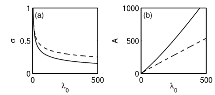
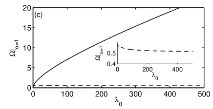
Fig. 1: Nonlocal model and variational approach: Solid lines show (a) width $\sigma$, (b) amplitude $A$, and (c) frequency $\Omega|_{\alpha=1}$ for the Bessel response as functions of the propagation constant $\lambda_{0}$. Dashed lines represent the same quantities for the Gaussian nonlocal response. The inset in (c) shows $\Omega|_{\alpha=1}$ for the latter response on more appropriate scales. While both, width $\sigma$ and amplitude $A$, exhibit similar behavior for the two nonlocal models the rotation frequency $\Omega|_{\alpha=1}$ shows a completely different dependence on $\lambda_{0}$ and drastic difference in magnitude for Gaussian and Bessel responses.

For the Bessel nonlocal response, Eq. (4), we have to compute the relevant integrals numerically. The results for both, Bessel and Gaussian models are presented in Fig. 1 using solid and dashed lines, respectively. It is clear that amplitude $A$ as well as soliton width $\sigma$, follow similar dependencies as a function of the propagation constant $\lambda_{0}$ [see Fig. 1(a-b)]. Totally different dependence shows the rotation frequency $\Omega$ [see Fig. 1(c)]. In particular, not only azimuthons in the Bessel nonlocal model rotate much faster than those predicted by the Gaussian model but also the former exhibit strong sensitivity of $\Omega$ on the propagation constant $\lambda$ and mass $M$.

To shed light on the origin of the difference in the rotating frequencies of the two models let us have a look at the quantities $M$ and $N_{\mathrm{cc}}-N_{\mathrm{cs}}$, which directly determine $\Omega|_{\alpha=1}$ in the present approximation [see Eq. (11)]. Figures 2(a,b) reveal that as the masses $M$ are comparable for both models, the important differences come from $N_{\mathrm{cc}}-N_{\mathrm{cs}}$. Hence, we can conclude that it is not the actual shape of the azimuthon which determines $\Omega$, but the convolution integrals $N_{\mathrm{cc}}$ and $N_{\mathrm{cs}}$ with the response function. In fact, $N_{\mathrm{cc}}$ and $N_{\mathrm{cs}}$ represent the overlaps of the nonlocal response of one dipole component with either itself or its $\pi/2$-rotated counterpart. Hence, the more of the non-rotational-symmetric shape is preserved by the nonlocal response, the larger is $N_{\mathrm{cc}}-N_{\mathrm{cs}}$. Looking at both response functions considered here in Fourier domain [Fig. 2(c)] it is obvious that the degree of nonlocality and consequently the degree of spatial averaging is greater for the Gaussian response leading to smaller difference between $N_{\mathrm{cc}}$ and $N_{\mathrm{cs}}$.

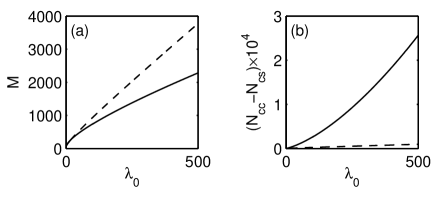
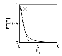
Fig. 2: (a) Mass $M$ and (b) quantity $N_{\mathrm{cc}}-N_{\mathrm{cs}}$ for Bessel (solid lines) and Gaussian (dashed lines) nonlocal responses as functions of the propagation constant $\lambda_{0}$. It is obvious that the difference in the rotating frequency $\Omega|_{\alpha=1}$ shown in Fig. 1(c) is due to $N_{\mathrm{cc}}-N_{\mathrm{cs}}$ [see Eq. (11)]. (c) Spatial Fourier Transform (FT) of the Bessel (solid lines) and Gaussian (dashed lines) nonlocal response $R$ as a function of the transverse wave-vector $k_{\perp}=\sqrt{k_{x}^{2}+k_{y}^{2}}$. The degree of spatial averaging is obviously larger for the Gaussian than for the Lorentzian.

4 Rotation Frequency - Numerical Analysis

How good are our approximations of the rotating frequency $\Omega$? Is the dependency in the structural parameter $\alpha$ really approximatively $\alpha/(\alpha^{2}+1)$ for a given $\lambda_{0}$? To answer these questions we compute the azimuthons $U$ numerically and propagate them over some distance in $z$ to observe their rotation and estimate $\Omega$. One typical example for the Gaussian nonlocal model is shown in Fig. 3. The corresponding vortex soliton has a propagation constant $\lambda_{0}=11.5$ and mass $M=200$. As its width $\sigma\approx 0.7$ is smaller than the width of the response function we are definitely in the nonlocal regime. We can clearly see the reasonable agreement between approximate and fully numerical results [compare with Fig. 1(c)]. We also tested azimuthons with larger masses and therefore corresponding to higher degrees of nonlocality. For instance, for $\lambda_{0}=247$, $M=2000$ and $\alpha=0.95$ we find $\Omega=0.54$ from direct numerical simulations, in excellent agreement with $\Omega=0.52$ from the approximate model [see also Fig. 1(c)]. Figure 4 shows another example, this time for the Bessel nonlocal model. Again, the agreement is reasonable. Here, we have to use higher $\lambda_{0}$ and larger mass in order to ensure the stability of the vortex soliton. Like in the previous example, we operate in a nonlocal regime ($\sigma=0.17$). To summarize, our simple approximate model for $\Omega$, which involves nothing but a variational solution for the vortex soliton, allows us to predict the correct range and sign of $\Omega$ for a family of dipole azimuthons with given mass. Moreover, the dependency on the structural parameter $\alpha$ is also correctly modeled.

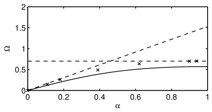
Fig. 3: Gaussian nonlocal model, $M=200$, $\lambda_{0}=11.5$: Solid line shows the result of Eq. (11) computed from the variational vortex approximation. Crosses depict results obtained from direct numerical solutions. Dashed lines represent results of the linear perturbation analysis of dipole and vortex soliton, respectively (see Sec. 5).

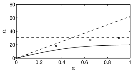
Fig. 4: Bessel nonlocal model, $M=2000$, $\lambda_{0}=418$: Same coding as in Fig. 3.

However, there is still serious discrepancy in the values of $\Omega|_{\alpha=1}$. One could think of two possible reasons. Firstly, it could be the deviations between the actual vortex soliton and its variational approximation. However, it turns out that $2(N_{\mathrm{cc}}-N_{\mathrm{cs}})/M$ computed from the numerically obtained vortex profile is almost constant (within a few percents). Hence it has no effect on the overall error in $\Omega|_{\alpha=1}$. However, postulating the specific ansatz Eq. (6) we implicitly assumed a certain shape of the deformation to the soliton profile while going over from the vortex to azimuthons, in the limit $\alpha\rightarrow 1$. Therefore it has to be this shape of vortex deformation which determines the rotation frequency $\Omega$, since a vortex formally allows for all possible rotations (see discussion on shifting $\lambda$ in end of Sec. 2). In the next section we will therefore discuss the formation of azimuthons by considering it as a process of bifurcation from the stationary non-rotating soliton solutions.

5 Internal Modes and Azimuthons

Let us start with the dipole soliton $D(r,\phi)$, because here the resulting linear problem is simpler than in the vortex case. We can directly use the rotation frequency $\Omega$ as the linearization parameter, since for the dipole we have $\Omega_{\mathrm{D}}=0$. We use the following ansatz

$$U(r,\phi-\Omega z)=D(r,\phi-\Omega z)+i\Omega d(r,\phi-\Omega z),$$ (15)

where $D$ and $d$ are real functions representing soliton and its small deformation, respectively. We then plug this ansatz into Eqs. (1), (5) and (6) and linearize with respect to $\Omega$. The resulting equation of order $\mathcal{O}(\Omega^{0})$ is fulfilled by the dipole soliton $D$. The terms of the order $\mathcal{O}(\Omega^{1})$ lead to the following linear equation for the deformation $d$:

$$-\lambda_{\mathrm{D}}d+\Delta_{\perp}d+\iint R(|\vec{r}-\vec{r}^{\prime}|)D^{2}(\vec{r}^{\prime})d^{2}\vec{r}^{\prime}d=\frac{\partial}{\partial\phi}D.$$ (16)

In deriving the above equation we made use of the fact that the propagation constant $\lambda$ of the azimuthon depends on $\Omega$ as $\lambda=\lambda_{\mathrm{D}}+\mathcal{O}(\Omega^{2})$, where $\lambda_{\mathrm{D}}$ is the propagation constant of the dipole soliton $D$. This can be seen easily from Eq. (7a) and $M=M_{\mathrm{D}}+\mathcal{O}(\Omega^{2})$, $L_{z}=0+\mathcal{O}(\Omega)$, $I=I_{\mathrm{D}}+\mathcal{O}(\Omega^{2})$, and $N=N_{\mathrm{D}}+\mathcal{O}(\Omega^{2})$, where the index ”${\mathrm{D}}$” indicates the respective integral for the dipole soliton $D$.

The solution of Eq.(16) for the Gaussian nonlocal model and the dipole soliton with $M=200$, and $\lambda_{D}=11.8$ is shown in Figure 5. The left plot shows the dipole soliton $D(x,y)$ while the right shows its deformation $d(x,y)$. As we can see from the right subplot, the deformation $d$ has a shape of a dipole as well, but rotated by $\pi/2$ with respect to $D$. The width of $d$ is about $0.85$ that of $D$. Hence, for small rotation frequency $\Omega$ the dipole azimuthon consists of two orthogonally oriented dipoles, with the the relative phase shift of $\pi/2$ and amplitude ratio $\alpha=\Omega\max d/\max D$. In effect, the whole rotating structure is slightly elliptic, with the principal axis given by $D$. In our example, we find $\max d/\max D=1.53$, hence $\Omega=1.53\alpha$, which agrees perfectly with exact numerical results obtained from the solution of the original nonlinear problem Eq.(1) for $\alpha\rightarrow 0$ (see Fig. 3).

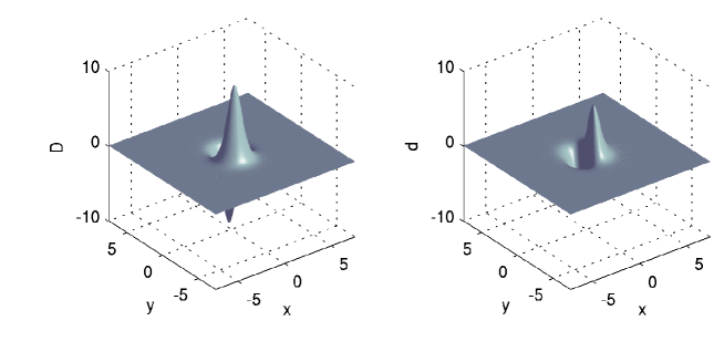
Fig. 5: Dipole $D$ and deformation $d$ for the Gaussian nonlocal model, $M=200$, $\lambda_{D}=11.8$. The deformation $d$ has a dipole shape, rotated by $\pi/2$ with respect to $D$. We can construct an approximate azimuthon $U=D+i\Omega d$ for small rotation frequencies $\Omega$. The amplitude ratio $\max d/\max D$ gives the slope of $\Omega(\alpha)$ at $\alpha=0$.

We obtain similar results for our second example, the dipole soliton in the Bessel nonlocal model with $M=2000$, $\lambda_{D}=444$ (see Fig. 6). The ratio of the widths of a dipole $D$ and its deformation $d$ is $0.76$, and $\Omega=62.1\alpha$. Again, the agreement with the full numerical results of Fig. 4 is excellent.

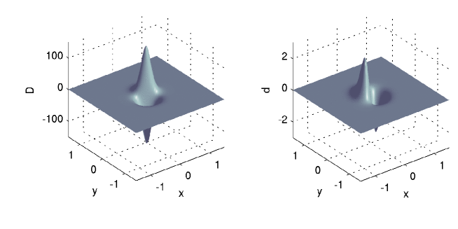
Fig. 6: Same as Fig. 5 but for the Bessel nonlocal model, $M=2000$, $\lambda_{D}=444$.

Let us now look at the azimuthon originating (bifurcating) from the vortex soliton. For this purpose, we recall the Eigenvalue problem for the internal modes of the nonlinear potential $\theta$ which is usually treated in the context of linear stability of nonlinear (soliton) solutions. We introduce a small perturbation $\delta V$ to the vortex soliton $V$, and plug

$$\psi=\left(V+\delta V\right)\mathrm{e}^{i\phi+i\lambda_{0}z}$$ (17)

into Eqs. (1) and (5) and linearize with respect to the perturbation. Please note that the perturbation $\delta V(r,\phi,z)$ is complex, whereas the vortex profile $V(r)$ can be chosen real. The resulting evolution equation for the perturbation $\delta V$ is given by

$$\begin{split}\left[i\frac{\partial}{\partial z}-\lambda_{0}+\frac{1}{r}\frac{\partial}{\partial r}\left(r\frac{\partial}{\partial r}\right)+\frac{1}{r^{2}}\left(\frac{\partial}{\partial\phi}+i\right)^{2}+\iint R(|\vec{r}-\vec{r}^{\prime}|)V^{2}(r^{\prime})d^{2}\vec{r}^{\prime}\right]\delta V&\\ +V\iint R(|\vec{r}-\vec{r}^{\prime}|)V(r^{\prime})\left[\delta V(\vec{r}^{\prime},z)+\delta V^{*}(\vec{r}^{\prime},z)\right]d^{2}\vec{r}^{\prime}&=0.\end{split}$$ (18)

With the ansatz

$$\delta V=\delta V_{1}(r)\mathrm{e}^{im\phi+i\kappa z}+\delta V^{*}_{2}(r)\mathrm{e}^{-im\phi-i\kappa^{*}z}$$ (19)

we then derive the Eigenvalue problem for the internal modes

$$\hat{L}\begin{pmatrix}\delta V_{1}\\ \delta V_{2}\end{pmatrix}=\kappa\begin{pmatrix}\delta V_{1}\\ \delta V_{2}\end{pmatrix},$$ (20)

where

$$\begin{split}\hat{L}\begin{pmatrix}\delta V_{1}\\ \delta V_{2}\end{pmatrix}&=\begin{pmatrix}\left[\frac{1}{r}\frac{\partial}{\partial r}\left(r\frac{\partial}{\partial r}\right)-\frac{(m+1)^{2}}{r^{2}}-\lambda_{0}+\iint R(|\vec{r}-\vec{r}^{\prime}|)V^{2}(r^{\prime})d^{2}\vec{r}^{\prime}\right]\delta V_{1}\\ -\left[\frac{1}{r}\frac{\partial}{\partial r}\left(r\frac{\partial}{\partial r}\right)-\frac{(m-1)^{2}}{r^{2}}-\lambda_{0}+\iint R(|\vec{r}-\vec{r}^{\prime}|)V^{2}(r^{\prime})d^{2}\vec{r}^{\prime}\right]\delta V_{2}\end{pmatrix}\\ &\quad+\begin{pmatrix}V\iint R(|\vec{r}-\vec{r}^{\prime}|)V(r^{\prime})\left[\delta V_{1}(r^{\prime})+\delta V_{2}(r^{\prime})\right]\cos[m(\phi-\phi^{\prime})]d^{2}\vec{r}^{\prime}\\ -V\iint R(|\vec{r}-\vec{r}^{\prime}|)V(r^{\prime})\left[\delta V_{2}(r^{\prime})+\delta V_{1}(r^{\prime})\right]\cos[m(\phi-\phi^{\prime})]d^{2}\vec{r}^{\prime}\end{pmatrix}.\end{split}$$ (21)

Real Eigenvalues of Eq. (20) ($\kappa=\kappa^{*}$) are termed orbitally stable and the corresponding Eigenvector $(\delta V_{1},\delta V_{2})$ can be chosen as real function. If we perturb the vortex $V$ with an orbitally stable Eigenvector, the resulting wave-function $\psi$ can be written in the form of Eq. (6) with $\Omega=-\kappa/m$ and $\lambda=\lambda_{0}-\kappa/m$. Hence, we expect to find an orbitally stable internal mode with $m=2$ corresponding to the azimuthon, where the Eigenvalue $\kappa$ gives $\Omega|_{\alpha=1}=-\kappa/2$.

Indeed, when we solve problem (20) for our two test cases numerically we find Eigenvalues at the expected positions, $\kappa=-1.4$ and $\kappa=-62$ respectively. The resulting estimates for $\Omega|_{\alpha=1}$ fit perfectly with values obtained from direct simulations (see Figs. 3 and 4). The radial profiles of the corresponding Eigenvectors are shown in Figs. 7 and 8). The total vorticity of the component $\sim\delta V_{1}$ is $2+1=3$, the one of $\sim\delta V_{2}$ is $-2+1=-1$. These total vorticities manifest themselves in the shapes of the radial profiles near the origin $r=0$.

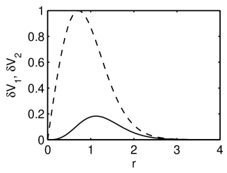
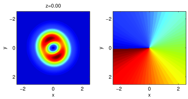
Fig. 7: Gaussian nonlocal model, $M=200$, $\lambda_{0}=11.5$: Solid line shows the component $\delta V_{1}$, dashed line the component $\delta V_{2}$, for $m=2$ and Eigenvalue $\kappa=-1.4$ computed from Eq. (20). The movie (4 MB or 15 MB) shows the evolution of intensity and phase of the vortex perturbed with the Eigenvector shown above, $U|_{z=0}=V\exp(i\phi)+\delta V_{1}\exp(i3\phi)+\delta V_{2}\exp(-i\phi)$. The chosen amplitudes of the perturbation are such that $\alpha=0.85$, the rotating frequency is close to $\Omega|_{\alpha=1}=0.7$.

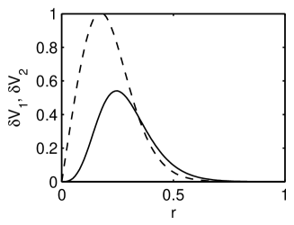
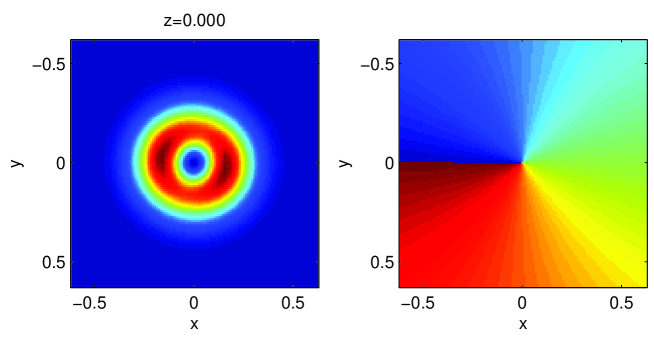
Fig. 8: Bessel nonlocal model, $M=2000$, $\lambda_{0}=418$: Same as in Fig. 7, $m=2$, $\kappa=-62$. The movie (4 MB or 15 MB) shows the evolution of the perturbed vortex with $\alpha=0.9$, the rotating frequency is close to $\Omega|_{\alpha=1}=31$.

As for the perturbation of the stationary dipole, it is possible to construct azimuthons in the vicinity of the vortex ($\alpha\approx 1$) from $\delta V$:

$$U(r,\phi)|_{z=0}=\left[V(r)+\delta V_{1}(r)\mathrm{e}^{im\phi}+\delta V_{2}(r)\mathrm{e}^{-im\phi}\right]\mathrm{e}^{i\phi}.$$ (22)

Used as an initial condition to the propagation equation this object is expected to rotate with $\Omega|_{\alpha=1}=-\kappa/m$. Unlike in the previous case of the stationary dipole, the amplitude of the perturbation is not fixed, but will eventually determine the value of the structural parameter $\alpha$. Generally speaking, the smaller the resulting $\alpha$ the greater the error in the constructed initial condition. However, the great robustness of the azimuthons allows one to use the initial condition (22) for quite large perturbation amplitudes (resulting $\alpha\sim 0.5$). Those ”bad” initial conditions result in oscillations of the azimuthon upon propagation. However, the azimuthon is structurally stable and does not decay into other solutions like the single-hump ground state. Moreover, such initial conditions play a role of excellent ”initial guesses” for solver routines to find numerically exact azimuthons. In the movies shown in Figs. 7 and 8 we choose moderate amplitudes of the perturbations in order to get almost perfect azimuthons. The corresponding structural parameters $\alpha\geq 0.85$ also guarantee that the observable rotating frequencies are very close to their limiting values $\Omega|_{\alpha=1}$.

The results of the linear stability analysis of the vortex soliton offer an easy explanation for the observed systematic deviation of the estimation for $\Omega|_{\alpha=1}$ by Eq. (11) from its true value. As mentioned before, the shape of the perturbation to the vortex soliton determines $\Omega|_{\alpha=1}$. In our ansatz (9) we only account for a perturbation similar to the component $\sim\delta V_{2}$ and ”forget” the other component $\sim\delta V_{1}$ with total vorticity 3, which leads to the observed deviation. The larger the ”forgotten” component, the larger is this deviation (compare Figs. 7, 3 and Figs. 8, 4).

There is more to say about the internal modes of the vortex soliton. On one hand, solving the Eigenvalue problem (20) for other vorticities $m$ offers an exhaustive method for finding families of azimuthons which originate from a vortex soliton. For example, with our method it was straightforward to identify a rotating triple-hump azimuthon ($m=3$, $\kappa=3.8$), which rotates with $\Omega=-\kappa/m=-1.27$. This solution bifurcate from the $M=200$ vortex in the Gaussian nonlocal model. The components of the generating Eigenvector are shown in Fig. 9. Again, we can easily construct various azimuthons with $\alpha\approx 1$ from this Eigenvector. The movie in Fig. 9 shows an example of the propagation of the triple-hump azimuthon with $\alpha=0.9$.

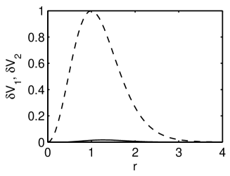
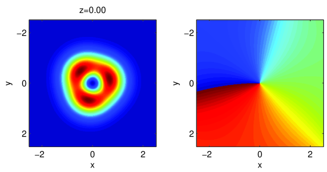
Fig. 9: Gaussian nonlocal model, $M=200$, $\lambda_{0}=11.5$: Same as in Fig. 7, $m=3$, $\kappa=3.8$. The movie (4 MB or 15 MB) shows the evolution of perturbed vortex $U|_{z=0}=V\exp(i\phi)+\delta V_{1}\exp(i4\phi)+\delta V_{2}\exp(-i2\phi)$, $\alpha=0.9$, the rotating frequency is close to $\Omega|_{\alpha=1}=-1.27$.

It should be stressed that not all orbitally stable Eigenvalues can be linked to a family of azimuthons. This is obvious for Eigenvalues with $|\kappa|>|\lambda_{0}|$ in the continuous part of the spectrum. Hence, we can conclude that $|\Omega|_{\alpha=1}|<|\lambda_{0}|/m$ for azimuthons bifurcating from a single-charged vortex. However, bound orbitally stable Eigenvalues do not necessary indicate an emanating family of azimuthons. For example, the $M=200$ vortex in the Gaussian nonlocal model possesses several other bounded internal modes for $m=2$, e.g. $\kappa=7$. If we perturb the vortex with the corresponding Eigenvector the resulting structure is a double-hump rotating with $\Omega=-3.5$. Closer inspection reveals that this structure decays and hence does not belong to another family of dipole azimuthons. Nevertheless, since those decaying rotating structures can survive over large propagation distances they may be indistinguishable from true azimuthons in the experimental conditions. This issue is currently under detailed investigation.

6 Conclusion

In conclusion, we analyzed properties of azimuthons, i.e. localized rotating nonlinear waves in nonlocal nonlinear media. We showed that the frequency of angular rotation crucially depends on the nonlocal response function. Starting with the single charge vortex soliton and by employing a simple variational ansatz we were able to predict accurately the frequencies of the rotating dipole azimuthon. In addition, we could explain how the actual shape of the response function determines the rotation frequencies. Further on, we computed exact dipole azimuthon solutions and their rotation frequencies numerically and showed that in the limits of maximal and/or minimal azimuthal amplitude modulation, i.e., close to the dipole or vortex soliton, the rotation frequency is determined uniquely by Eigenvalues of the bound modes of the linearized version of the respective stationary nonlocal solution. Moreover, the intensity profile of the resulting azimuthon can be constructed from the corresponding linear Eigen-solution. This offers a straightforward and exhaustive method to identify rotating soliton solutions in a given nonlinear medium.

7 Acknowledgment

This research was supported by the Australian Research Council. Numerical simulations were performed on the SGI Altix 3700 Bx2 cluster of the Australian Partnership for Advanced Computing (APAC).