HISKP-TH-08/07
A Model Study of Discrete Scale Invariance and Long-Range Interactions

Abstract

We investigate the modification of discrete scale invariance in the bound state spectrum by long-range interactions. This problem is relevant for effective field theory descriptions of nuclear cluster states and manifestations of the Efimov effect in nuclei. As a model system, we choose a one dimensional inverse square potential supplemented with a long-range Coulomb interaction. We study the renormalization and bound-state spectrum of the system as a function of the Coulomb interaction strength. Our results indicate, that the counterterm required to renormalize the inverse square potential alone is sufficient to renormalize the full problem. However, the breaking of the discrete scale invariance through the Coulomb interaction leads to a modified bound state spectrum. The shallow bound states are strongly influenced by the Coulomb interaction while the deep bound states are dominated by the inverse square potential.

1 Introduction

The application of effective field theory (EFT) methods to nuclear physics is by now well established Bedaque:2002mn . If there is a separation of scales in a physical system, effective field theory allows for controlled calculations of low-energy observables with well-defined error estimates. In nuclear physics, mostly effective field theories with nucleons and pions (and possibly Deltas) as degrees of freedom are used. However, for a certain class of systems, it is possible to use effective field theories with even more effective degrees of freedom Braaten:2004rn . This is the realm of halo nuclei and nuclear cluster states.

A halo nucleus is one that consists of a tightly bound core surrounded by one or more loosely bound valence nucleons. The valence nucleons are characterized by a very low separation energy compared to those in the core. As a consequence, the radius of the halo nucleus is large compared to the radius of the core. The separation of scales in halo nuclei leads to universal properties that are insensitive to the structure of the core (see, e.g., Ref. DFHT00 and references therein). The most carefully studied Borromean halo nuclei are ⁶He and ¹¹Li, which have two weakly bound valence neutrons ZDFJV93 ; JRFG04 . In the case of ⁶He, the core is an alpha particle. An EFT framework to describe halo systems was introduced in BHvK1 ; BHvK2 where the neutron-alpha ($n\alpha$) system was studied in an EFT with nucleon and alpha degrees of freedom. Further extensions to the proton-alpha and alpha-alpha systems were considered in Refs. BRvK ; Higa:2008dn . Similar concepts can be applied to nuclear cluster states. The best-known example is the structure of ¹²C. This system has an excited $0^{+}$ state, the so-called Hoyle state which shows a clear clustering into three $\alpha$ particles. This observation suggests that this state can be described by an EFT of $\alpha$ particles inteacting via short-range contact interactions. An important question is whether there is an universal binding mechanism for these systems. A prime candidate for such a mechanism is the Efimov effect Efimov70 .

In an EFT framework, the Efimov effect can be related to a renormalization group (RG) limit cycle Albe-81 . Most applications of the RG involve a flow towards a fixed point, where the system is scale invariant. However, as pointed out by Wilson Wilson:1970ag , one can also have closed curves under the RG flow in the space of coupling constants. The RG flow completes a cycle around the curve every time the cutoff is changed by a multiplicative factor $\lambda_{0}$. This number $\lambda_{0}$ is the preferred scaling factor. A necessary condition for a limit cycle is invariance under discrete scale transformations: $x\to\lambda_{0}^{n}x$, where $n$ is an integer. This discrete scaling symmetry is reflected in log-periodic behavior of physical observables. The Efimov effect can be understood as the manifestation of a limit cycle in the bound state spectrum of the three-body problem with large scattering length $a$. This limit cycle property is manifest in the EFT treatment of Refs. Bedaque:1998kg , where an explicit log-periodic three-body counterterm is introduced. In the limit $a\to\pm\infty$, there is an accumulation of 3-body bound states near threshold with binding energies differing by multiplicative factors of $\lambda_{0}^{2}\simeq 515.03$ Efi71 . Recently, the first convincing experimental evidence for this effect was obtained by measuring its effect on three-body loss rates in a gas of cold Cs atoms Grimm06 .

The Efimov effect could also be responsible for the binding of certain halo nuclei and cluster states Federov:1994cf . In particular for the latter, however, the short-range strong interaction is usually accompanied by a long-range Coulomb interaction. The effect of such long-range Coulomb interactions on the physics of limit cycles and discrete scale invariance is therefore an important issue. In order to get some insight into this question, we start with a simpler problem that has also a limit cycle behavior: the one-dimensional Schrödinger equation with an attractive inverse square potential. If the attraction is larger than a certain critical value, the system also shows a limit cycle. This limit cycle becomes evident in a bound state spectrum with discrete scale invariance similar to the Efimov effect. Indeed, the inverse square potential is intimitely connected to the three-body system with large scattering length, which reduces to a one-dimensional Schrödinger equation with an inverse square potential in the hyperradius for large momenta Efi71 ; Braaten:2004rn . This makes the inverse square potential an ideal model system to study the physics of limit cycles and discrete scale invariance Beane:2000wh ; Bawin:2003dm ; Braaten:2004pg ; Barford:2004fz ; Hammer:2005sa ; long-2007 .

In this paper, we study the effect of a long-range Coulomb interaction on discrete scale invariance in the bound state spectrum for an inverse square potential with a Coulomb potential. (For an earlier study of the interplay between Coulomb and strong interactions in exotic atoms, see Ref. Gal96 .) In the next section, we briefly review the renormalization of the inverse square potential in the approach of Ref. Hammer:2005sa . In Sec. 3, we introduce the long-range Coulomb potential. The renormalization and our results for the bound state spectrum are discussed in Sec. 4 and in Sec. 5 a perturbative treatment of the Coulomb interaction is given. Finally, we present our conclusions in Sec. 6. Our treatment of the Coulomb divergence is described in Appendix A.

2 Inverse Square Potential

In order to set up our problem, we briefly review the renormalization of the $1/r^{2}$ potential in momentum space without the long-range Coulomb interaction Hammer:2005sa . We consider the attractive inverse square potential

$$V_{S}(r)=\frac{\hbar^{2}}{m}\frac{c}{r^{2}}\,,\qquad\mbox{with}\quad r\equiv|\vec{r}|\,,\quad c\equiv-\frac{1}{4}-\nu^{2}\,,$$ (1)

and $\nu>0$ a positive real parameter. This potential has the same scaling behavior as the kinetic energy operator and, consequently, is scale invariant at the classical level. In the following, we set the particle mass and Planck’s constant $m=\hbar=1$ for convenience. For values of $c\geq-\frac{1}{4}$, the potential is well-behaved and the corresponding Schrödinger equation has a unique solution, see Ref. FLS71 . However, we are interested in the case $c<-\frac{1}{4}$ which corresponds to real values of $\nu$ in (1). In this case, the $1/r^{2}$ potential is singular and the usual boundary conditions for the Schrödinger equation do not lead to a unique solution. We can calculate the Fourier transform of the potential using dimensional regularization (see Ref. Hammer:2005sa for details). This leads to the expression

$$V_{S}(q)=\frac{2\pi^{2}c}{q}\,$$ (2)

for the momentum space representation of the $1/r^{2}$ potential (1). Since the potential is local, its Fourier transform depends only on the momentum transfer $q$.

The Lippmann-Schwinger (LS) equation for two particles interacting via $V_{S}(q)$ from Eq. (2) in their center-of-mass frame takes the form

$$T_{E}(\vec{p},\vec{p}^{\prime})=V_{S}(|\vec{p}-\vec{p}^{\prime}|)+\int\frac{d^{3}q}{(2\pi)^{3}}\frac{V_{S}(|\vec{p}-\vec{q}|)}{E-q^{2}+i\epsilon}\,T_{E}(\vec{q},\vec{p}^{\prime})\,,$$ (3)

where $E$ is the total energy and $\vec{p}$ ($\vec{p}^{\prime}$) are the relative momenta of the incoming (outgoing) particles, respectively. A pictorial representation of this equation is given in Fig. 1.

Figure 1: Lippmann-Schwinger equation for a two-body potential $V$.

We are only interested in the S-wave contribution. In higher partial waves the singular behavior of the potential is screened by the angular momentum barrier, but for sufficiently strong attraction it will become visible as well (see, e.g., Ref. long-2007 ). Projecting onto S-waves by integrating the equation over the relative angle between $\vec{p}$ and $\vec{p}^{\prime}$: $\frac{1}{2}\,\int d\cos\theta_{\vec{p}\vec{p}^{\prime}}$, we obtain the integral equation

$$t_{E}(p,p^{\prime}) = v_{S}(p,p^{\prime})+\frac{1}{2\pi^{2}}\int_{0}^{\infty}\frac{dq\,q^{2}}{E-q^{2}+i\epsilon}$$ (4)

$$\times\,v_{S}(p,q)\,t_{E}(q,p^{\prime})\,,$$

where

$$v_{S}(p,q)=2\pi^{2}c\left(\frac{\theta(p-q)}{p}+\frac{\theta(q-p)}{q}\right)\,.$$ (5)

The physical observables are the bound state spectrum and the scattering phase shifts $\delta(k)$. The phase shifts are determined by the solution to Eq. (4) evaluated at the on-shell point $E=k^{2}$, $k=p^{\prime}=p$ via $t_{k^{2}}(k,k)=-4\pi/(k\cot\delta(k)-ik)$ . Since $p^{\prime}$ appears only as a parameter in Eq. (4), we can set $p^{\prime}=p$ to simplify the equation. The binding energies are given by those values of $E<0$ for which the homogeneous version of Eq. (4) has a solution. For the bound state equation the dependence of the solution $\phi_{E}(p)$ on $p^{\prime}$ disappears altogether.

It is well-known that Eq. (4) does not have a unique solution since the $1/r^{2}$ potential for real $\nu$ is singular FLS71 . The most general solution of the bound state equation for $E=0$ can be written as

$$\phi_{0}(p)={\cal N}\,p^{-1/2}\left(p^{i\nu}e^{i\varphi}+p^{-i\nu}e^{-i\varphi}\right)\,,$$ (6)

where the relative phase $\varphi$ is a free parameter. The value of $\varphi$ is not determined by the $1/r^{2}$ potential and has to be taken from elsewhere. It is exactly this phase $\varphi$ which is fixed by self-adjoint extensions of the potential Bawin:2003dm .

In the framework of an effective theory, this is conveniently done using renormalization theory. We regularize the LS equation by applying a momentum cutoff $\Lambda$ and include a momentum-independent counterterm $\delta V_{S}(\Lambda)$ in the potential. The precise form of the cutoff, for example Gaussian cutoff or sharp cutoff, is not important, but we use a sharp cutoff for simplicity. Making the replacement

$$V_{S}(q)\quad\Rightarrow\quad V_{S}(q)+\delta V_{S}(\Lambda)=\frac{2\pi^{2}c}{q}+\frac{H_{S}(\Lambda)}{\Lambda}\,$$ (7)

in Eq. (3) the LS equation (4) for bound state solutions with $E=-E_{B}<0$ becomes

$$\phi_{E_{B}}(p) = -\frac{1}{2\pi^{2}}\int_{0}^{\Lambda}\frac{dq\,q^{2}}{E_{B}+q^{2}}$$ (8)

$$\times\left[v_{S}(p,q)+\frac{H_{S}(\Lambda)}{\Lambda}\right]\,\phi_{E_{B}}(q)\,.$$

The functional dependence of $H_{S}(\Lambda)$ can be determined analytically from invariance of low-energy observables under renormalization group transformations. We demand that the relative phase of the zero-energy bound solution of Eq. (8) remains unchanged under variations of the cutoff $\Lambda$ and find

$$H_{S}(\Lambda)=2\pi^{2}c\,\frac{1-2\nu\tan(\nu\ln(\Lambda/\Lambda_{*}))}{1+2\nu\tan(\nu\ln(\Lambda/\Lambda_{*}))}\,,$$ (9)

where $\Lambda_{*}$ is a free parameter that determines the relative phase in (6): $\varphi=-\nu\ln\Lambda_{*}$. In order to fix $\varphi$, we can either specify both the cutoff $\Lambda$ and the dimensionless coupling $H$ or, using Eq. (9), one dimensionful parameter: $\Lambda_{*}$. This parameter $\Lambda_{*}$ is generated by the iteration of quantum corrections in solving the integral equation (8). This is similar to the phenomenon of dimensional transmutation in QCD Wil99 .

Note that $H_{S}(\Lambda)$ remains unchanged when the argument is multiplied by $\lambda_{0}^{n}$, where $n$ is an integer number and $\lambda_{0}=e^{\pi/\nu}$ is the discrete scaling factor. This discrete scaling symmetry is a consequence of the limit cycle and reflects itself in physical observables Braaten:2004rn ; Hammer:2005sa . In the bound state spectrum, for example, the ratio of consecutive binding energies is a constant, $E_{n}/E_{n+1}=\lambda_{0}^{2\pi/\nu}$. Therefore, we can study modifications of the limit cycle through modifications to the discrete scaling symmetry of the bound state spectrum.

Moreover, the discrete symmetry implies the existence of a set of cutoffs

$$\Lambda_{n}(\Lambda_{*})=\Lambda_{*}\exp(n\pi/\nu)\,$$ (10)

with $H_{S}(\Lambda_{n})\equiv 0$. We can therefore obtain a renormalized version of Eq. (8) that does not explicitly contain the counterterm by using the discrete set of cutoffs from Eq. (10). The same trick can be used for the three-body problem with large scattering length Hammer:2000nf .

3 Inclusion of the Long-Range Potential

We now include an additional attractive Coulomb potential of the form

$$V_{C}(q)=-\frac{4\pi\alpha}{q^{2}+\gamma^{2}}\,,$$ (11)

where $\gamma$ is a photon mass that will be taken to zero in the end. The speed of light has been set to unity for convenience. In the following, we vary the strength $\alpha$ of the potential. Projecting onto S-waves as discussed in the previous section we find

$$v_{C}(p,q)=-\frac{\pi\alpha}{pq}\ln\left[\frac{(p+q)^{2}+\gamma^{2}}{(p-q)^{2}+\gamma^{2}}\right]\,.$$ (12)

The integral equation for bound state solutions, Eq. (8), then becomes

$$\phi_{E_{B}}(p) = -\frac{1}{2\pi^{2}}\int_{0}^{\Lambda}\frac{dq\,q^{2}}{E_{B}+q^{2}}\,\bigg{[}v_{S}(p,q)$$ (13)

$$\quad+\frac{H_{S}(\Lambda)}{\Lambda}+v_{C}(p,q)\bigg{]}\,\phi_{E_{B}}(q)\,.$$

From Eq. (12), it is clear that the kernel of the integral equation (13) diverges for $q=p$ in the limit $\gamma\to 0$: this is the well-known Coulomb singularity. Its origin can be traced back to the integral equation for the scattering amplitude with a long-range Coulomb interaction, which diverges at forward angles. When projected into S-waves, this singularity appears in the diagonal terms of the potential in momentum space. For the binding energies this singularity should not be a problem, as long as the diagonal terms are handled properly. In Appendix A, we describe how to treat these terms, based on the the idea outlined in Ref. Coultrick .

4 Renormalization and Results

First we address the renormalization of the full problem including Coulomb. It is not clear a priori whether the introduction of the Coulomb potential will require an additional counterterm.

In order to answer this

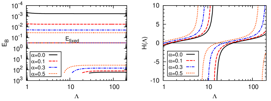
Figure 2: Bound state spectrum with one state fixed at $E_{B}\approx 0.308$ (left panel) and the counterterm required for renormalization (right panel) for $\alpha=0,0.1,0.3,0.5$ and with $\nu=\Lambda_{*}=1$, as a function of $\Lambda$. In the right panel, the curve $\alpha=0$ coincides with $H(\Lambda)$ given by Eq. (9), except for $\Lambda\lesssim 1$.

question, we calculate the bound state spectrum at a given cutoff and choose to fix the binding energy of one bound state as the cutoff $\Lambda$ is varied. The fixed energy was chosen as one of the pure $1/r^{2}$ states, $E_{\rm fixed}\approx 0.308$. We then calculate the bound state spectrum for other values of the cutoff $\Lambda$ and adjust the counterterm $H_{S}(\Lambda)$ numerically to keep this binding energy fixed. The results of this analysis are shown in Fig. 2. The left panel shows the bound states for $\alpha=0,0.1,0.3,0.5$ as a function of $\Lambda$. In order to keep this and the remaining figures as legible as possible, only the three deepest states are shown. The case $\alpha=0$ corresponds to the pure $1/r^{2}$ potential. One observes that the cutoff dependence of all states is removed once the counterterm is adjusted to fix one of the states. Note, however, that the deepest state shows a cutoff dependence near the cutoff where it first appears with infinite binding energy. This behavior has nothing to do with the long-range interaction and is due to the way the system is renormalized, keeping low-energy physics unchanged. A similar behavior is also observed for the pure $1/r^{2}$ potential and the three-body system with large scattering length Bedaque:1998kg ; Braaten:2004pg ; Hammer:2005sa .

Moreover, it is evident that the long-range interaction destroys the discrete scale invariance in the spectrum. Only for $\alpha=0$, the ratio of consecutive binding energies is a constant. In the right panel of Fig. 2, we show the numerically determined values of the counterterm $H_{S}(\Lambda)$ as a function of $\Lambda$ for $\alpha=0,0.1,0.3,0.5$. The figure suggests that the long range potential shifts the argument of the counterterm $H_{S}(\ln\Lambda)\to H_{S}(\ln\Lambda+f(\alpha))$ where $f(\alpha)$ is a monotonic function of the coupling $\alpha$. This implies that the long-range Coulomb potential merely renormalizes the value of $\Lambda_{*}$. As a consequence, the counterterm $H_{S}(\Lambda)$ from Eq. (9) should be sufficient to renormalize Eq. (13) including the long-range Coulomb potential.

In order to test this assumption, we calculate the bound state spectrum using the counterterm for the pure $1/r^{2}$ potential from Eq. (9). The result is shown in Fig. 3. For simplicity, we take $\nu=\Lambda_{*}=1$ and show different values of $\alpha$. For each energy level, the binding energies increase as the Coulomb strength is increased. It is evident that the Coulomb potential influences the spectrum, but does not destroy the cutoff independence of the binding energies. Clearly, no additional counterterm is required.

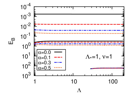
Figure 3: Binding energies for $\nu=\Lambda_{*}=1$ as function of the cutoff $\Lambda$ for $\alpha=0,0.1,0.3,0.5$.

Note also that the shift in energy due to the Coulomb interaction depends on the exitation level — the deepest bound states have the smallest shifts relative to the pure $1/r^{2}$ case, while the shallower ones have larger shifts and resemble more the Coulomb spectrum. This behavior can be understood by comparing the relative strengths of the $1/r^{2}$ and $1/r$ potentials in coordinate space. There will always be a special distance $\bar{r}=|c|/\alpha=(1/4+\nu^{2})/\alpha$ where the two potentials have equal strength: $V_{S}(\bar{r})=V_{C}(\bar{r})$. The qualitative pattern of the energy levels can be understood by comparing the binding energy of a given state, $E_{B}$, with the potential energy at $\bar{r}$,

$${\bar{E}}_{\rm pot}=|V_{S}(\bar{r})+V_{C}(\bar{r})|=\frac{2\alpha^{2}}{1/4+\nu^{2}}\,.$$ (14)

The bound states with $E_{B}\gg{\bar{E}}_{\rm pot}$ are more sensitive to shorter distances where $V_{S}$ dominates over $V_{C}$. Therefore, the spectrum resembles the $1/r^{2}$ spectrum and is approximately scale invariant. For $E_{B}\ll E_{\rm pot}$, on the other hand, the states are more sensitive to larger distances and the spectrum is similar to the Coulomb spectrum.

An alternative way of understanding this behavior is by looking at Eq. (13). We take one of the bound states $E_{B}=B_{n+1}$ with an eigensolution $\phi_{n+1}(p)$. The next deeper bound state, denoted by $B_{n}$, defines a variable $t_{n}$ ($>1$) via $t_{n}^{2}=B_{n}/B_{n+1}$. $B_{n}$ has an eigensolution $\phi_{n}(p)$ that satisfies

$$\phi_{n}(p) = -\frac{1}{2\pi^{2}}\int_{0}^{\Lambda}\frac{dq\,q^{2}}{B_{n}\!+\!q^{2}}\bigg{\{}2\pi^{2}c\bigg{[}\frac{\theta(p\!-\!q)}{p}+\frac{\theta(q\!-\!p)}{q}\bigg{]}$$ (15)

$$+\frac{H_{S}(\Lambda/\Lambda_{*})}{\Lambda}-\frac{\pi\alpha}{pq}\ln\bigg{[}\frac{(p\!+\!q)^{2}}{(p\!-\!q)^{2}}\bigg{]}\bigg{\}}\phi_{n}(q),$$

where we explicitly indicated the dependence of $H_{S}$ on $\Lambda$ and $\Lambda_{*}$. Rescaling the external momentum $p$ and the integration variable $q$ by $t_{n}$ yields

$$\phi_{n}(t_{n}p) = -\frac{1}{2\pi^{2}}\int_{0}^{\Lambda}\frac{dq\,q^{2}}{B_{n}/t_{n}^{2}\!+\!q^{2}}\times$$ (16)

$$\bigg{\{}2\pi^{2}c\bigg{[}\frac{\theta(p\!-\!q)}{p}+\frac{\theta(q\!-\!p)}{q}\bigg{]}+\frac{H_{S}(t_{n}\Lambda/\Lambda_{*})}{\Lambda}$$

$$-\frac{1}{t_{n}}\frac{\pi\alpha}{pq}\ln\bigg{[}\frac{(p\!+\!q)^{2}}{(p\!-\!q)^{2}}\bigg{]}\bigg{\}}\phi_{n}(t_{n}q).$$

In addition, we set $\Lambda\to t_{n}\Lambda$ assuming cutoff independence, which is verified numerically. Writing $t_{n}=\exp(\pi/\nu+\delta_{n})$ and using the log-periodicity of $H_{S}$, we conclude from Eq. (16) that $B_{n+1}$ is also a bound state of a Hamiltonian that has a Coulomb potential weakened by $1/t_{n}$ and parameter $\Lambda_{*}$ multiplied by $e^{-\delta_{n}}$. By induction, it follows that a deeper state $B_{n-k}$, with eigensolution $\phi_{n-k}(p)$, is given by $\sigma_{k}B_{n+1}=(\Pi_{j=0}^{k-1}t_{n-j})B_{n+1}$. Furthermore, $B_{n+1}$ is an eigenvalue, with eigensolution $\phi_{n-k}(\sigma_{k}p)$, of the Hamiltonian $H_{0}+V_{S}+V_{C}/\sigma_{k}$ with a parameter $\Lambda_{*}$ multiplied by $e^{-\Delta_{k}}=\exp(-\sum_{j=0}^{k-1}\delta_{n-j})$. Therefore, the solution $\phi_{n-k}(p)$ with eigenvalue $B_{n-k}$ is only weakly sensitive to the Coulomb potential. The same rationale applies to the solution $\phi_{n-k-1}(p)$ for the next deeper state $B_{n-k-1}$. One therefore expects that $\delta_{n-k-1}$ tends to zero and, consequently, $t_{n-k-1}$ to the discrete scaling factor $e^{\pi/\nu}$.

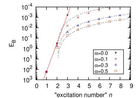
Figure 4: Binding energies for $\nu=\Lambda_{*}=1$ and $\alpha=0,0.1,0.3,0.5$ as function of the “exitation number” $n$ (see text for details).

In order to support these conclusions, we plot in Fig. 4 the binding energies as functions of the “excitation number” $n$, the latter being defined relative to the deepest bound state at $\Lambda=200$. For $\nu=1$ and $\alpha=0.1,0.3,0.5$, one has ${\bar{E}}_{\rm pot}=1.6\times 10^{-2},1.44\times 10^{-1},4.0\times 10^{-1}$, respectively. The exact scale invariance is broken for any finite value of $\alpha$. The figure illustrates how the limit of exact discrete scale invariance is approached as the states become deeper. It confirms that for $E_{B}\gg{\bar{E}}_{\rm pot}$ the behavior is closer to the geometric $1/r^{2}$ spectrum with $\ln E_{B}={\rm const.}+n\times 2\pi/\nu$. This spectrum is indicated by the solid straight line. For large $n$, where ${\bar{E}}_{B}\ll E_{\rm pot}$, the spectrum approaches the Coulomb spectrum. This is illustrated by the dotted lines which represent the Coulomb energies $\alpha^{2}/(4\tilde{n}^{2})$, with the shifted excitation number $\tilde{n}=n-2$. This particular choice of $\tilde{n}$ is natural since the $n=3$ level is the closest to the $n=1$ level of the pure-Coulomb spectrum. In accordance with our expectations, the Coulomb pattern is already observed at moderate $n$ for $\alpha=0.5$ and $0.3$, while it is achieved at larger $n$ for $\alpha=0.1$.

Next we study the dependence of the bound state spectrum on $\nu$ and $\Lambda_{*}$. In Fig. 5, we show the spectra for $\nu=1$ and $\Lambda_{*}=2$ (left panel) and for $\Lambda_{*}=1$ and $\nu=2$ (right panel). We first consider the left panel. Due to the discrete scale invariance, a change of $\Lambda_{*}$ in the pure $1/r^{2}$ case modifies the values of the energies but preserves the geometric character of the spectrum, i.e. the ratio of subsequent states is determined by the preferred scaling factor squared $(e^{\pi/\nu})^{2}$. This behavior is manifest as a vertical displacement of the spectrum $\alpha=0$ relative to the one shown in Fig. 3.

 

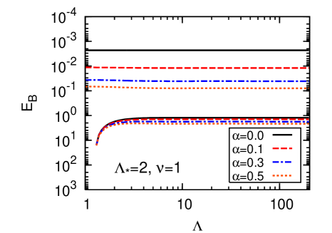
Figure 5: Bound state spectrum for $\Lambda_{*}=2$ and $\nu=1$ (left panel) and for $\Lambda_{*}=1$ and $\nu=2$ (right panel).

A similar shift of the energies is also expected for $\alpha\neq 0$. However, the Coulomb interaction breaks the discrete scale invariance and modifies the ratios between consecutive energy levels. The increase of $\Lambda_{*}$ provides more binding to the system, while the splitting among different values of $\alpha$ is reduced. This observation is in agreement with the finding in the previous section: deeper bound states become less sensitive to the Coulomb part of the interaction, which is responsible for the different splittings. Next we consider the case $\Lambda_{*}=1$ and $\nu=2$ shown in the right panel of Fig. 5. For a given value of $\alpha$, the $1/r^{2}$ part of the interaction becomes relatively stronger and the overall binding is increased. The influence of the long-range Coulomb part is decreased. For the pure $1/r^{2}$ case $\alpha=0$, the discrete scaling factor is reduced to $e^{\pi/2}$ and the states move closer together. For the case $\alpha\neq 0$, the spectrum has distinct features of the $1/r^{2}$ problem — very little spread in energy among the different $\alpha$ considered, and a binding ratio very close to $(e^{\pi/2})^{2}$.

5 Perturbative Treatment of the Coulomb Part

In the previous section we saw that the deepest bound states have small Coulomb corrections. In this section we calculate these energy shifts relative to the unperturbed $1/r^{2}$ solution in perturbation theory in order to test our hypothesis.

It is convenient to start from the LS equation for the scattering state instead of the transition amplitude (3). The former reads

$$|\Psi_{p}^{(\pm)}\rangle=|\vec{p}\rangle+G_{0}^{(\pm)}(E)\left(\hat{V}_{S}+\lambda\hat{V}_{C}\right)|\Psi_{p}^{(\pm)}\rangle\,,$$ (17)

where $|\Psi_{p}^{(+)}\rangle$ ($|\Psi_{p}^{(-)}\rangle$) is the initial (final) state, $G_{0}^{(\pm)}(E)$ is the free two-particle propagator, and $\lambda$ is a parameter expansion that will be set to 1 in the end. Expanding the scattering state and the binding energy in powers of a small parameter $\lambda$,

$$|\Psi_{p}^{(\pm)}\rangle = |\chi_{p}^{(\pm)}\rangle+\lambda\,|\varphi_{p}^{(\pm)}\rangle+\cdots\,,$$

$$E = E^{(0)}+\lambda\,E^{(1)}+\cdots\,,$$ (18)

one gets to leading order in $\lambda$ the LS equation for the pure $1/r^{2}$ interaction $\hat{V}_{S}$:

$$|\chi_{p}^{(+)}\rangle=|\vec{p}\rangle+G_{0}^{(+)}(E^{(0)})\,\hat{V}_{S}\,|\chi_{p}^{(+)}\rangle\,.$$ (19)

Multiplication of this equation by $\langle\vec{p}^{\prime}|\hat{V}_{S}$ gives the LS equation for $T_{E}(\vec{p},\vec{p}^{\prime})\equiv\langle\vec{p}^{\prime}|\hat{V}_{S}|\chi_{p}^{(+)}\rangle$ (cf. Eq. (3)). Collecting the terms linear in $\lambda$, we obtain

$$|\varphi_{p}^{(+)}\rangle = \left[G_{0}^{(+)}(E^{(0)})\,\hat{V}_{C}-E^{(1)}\,G_{0}^{(+)}(E^{(0)})^{2}\,\hat{V}_{S}\right]|\chi_{p}^{(+)}\rangle$$ (20)

$$+G_{0}^{(+)}(E^{(0)})\,\hat{V}_{S}\,|\varphi_{p}^{(+)}\rangle\,.$$

This is an integral equation for the state $|\varphi_{p}^{(+)}\rangle$ with a driving term proportional to the unperturbed state $|\chi_{p}^{(+)}\rangle$. Since we are dealing with bound states, one can use the homogeneous version of Eq. (19) to eliminate the state $|\varphi_{p}^{(+)}\rangle$ from the above equation. This is achieved via multiplication from the left by $\langle\chi_{p^{\prime}}|\hat{V}_{S}$ and yields

$$\langle\chi_{p^{\prime}}^{(+)}|\hat{V}_{S}\,G_{0}^{(+)}(E^{(0)})\,\hat{V}_{C}|\chi_{p}^{(+)}\rangle$$

$$-E^{(1)}\langle\chi_{p^{\prime}}^{(+)}|\hat{V}_{S}\,G_{0}^{(+)}(E^{(0)})^{2}\,\hat{V}_{S}|\chi_{p}^{(+)}\rangle=0\,.$$ (21)

We can again use Eq. (19) to express $E_{B}^{(1)}=-E^{(1)}$ in terms of the transition amplitude $T_{E}(\vec{p},\vec{p}^{\prime})$ defined by Eq. (3). After integration over the angles, we obtain

$$E_{B}^{(1)}=-A/B$$ (22)

where

$$A = \int_{0}^{\Lambda}dp\int_{0}^{\Lambda}dq\,\frac{p^{2}\phi^{(0)}(p)}{E_{B}^{(0)}\!+\!p^{2}}\,v_{C}(p,q)\,\frac{q^{2}\phi^{(0)}(q)}{E^{(0)}_{B}\!+\!q^{2}}\,,$$

$$B = 2\pi^{2}\int_{0}^{\Lambda}dp\,\frac{p^{2}\phi^{(0)}(p)^{2}}{(E_{B}^{(0)}\!+\!p^{2})^{2}}\,,$$ (23)

and $\phi^{(0)}(p)$ is the solution of Eq. (8).

 

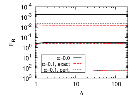
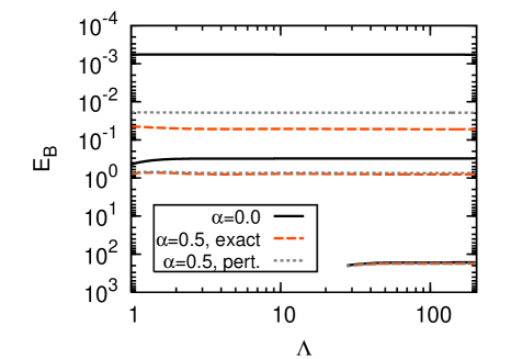
Figure 6: Bound state spectrum with a perturbative Coulomb treatment for $\alpha=0.1$ (left panel) and $\alpha=0.5$ (right panel), compared against the exact and $\alpha=0$ cases. The parameters $\Lambda_{*}$ and $\nu$ were set to 1.

A comparison of the exact binding energies with the perturbative results is given in Fig. 6. We show the perturbative Coulomb binding energies for $\alpha=0.1$ (left panel) and $0.5$ (right panel), compared with exact energies and the energies for the pure $1/r^{2}$ case. On one hand one clearly sees that the perturbative treatment works quite well for the two deepest bound states, where the effect of the Coulomb interaction is expected to be small. This is true even for a relatively strong Coulomb potential with $\alpha=0.5$. The shallowest state in Fig. 6, on the other hand, cannot be described by perturbation theory in the Coulomb potential. In this case, we no longer have $E_{B}\gg{\bar{E}}_{\rm pot}$ (cf. Eq. (14)) and the Coulomb effects are large. Indeed, the perturbative treatment of the Coulomb interaction gives $4.4\times 10^{-3}$ ($1.9\times 10^{-2}$) compared to the exact value $6.3\times 10^{-3}$ ($5.2\times 10^{-2}$), for $\alpha=0.1$ ($\alpha=0.5$). These results clearly support our hypothesis from the previous section.

We should point out that a perturbative treatment of the $1/r^{2}$ potential relative to the Coulomb potential to calculate the shallower states is not possible. This is due to the singular nature of the $1/r^{2}$ potential for real values of $\nu$ in Eq. (1) which we consider here. We have verified explicitly that if the $1/r^{2}$ potential is not singular (corresponding to imaginary $\nu$) the perturbative treatment works quite well. The latter case, however, corresponds to a situation where the Schrödinger equation has a unique solution and limit cycles are absent.

6 Summary and Conclusions

In this work, we have investigated the modification of limit cycles and discrete scale invariance by the presence of a long-range interaction. As a specific example, we have considered the quantum mechanical inverse square potential supplemented by an attractive long-range Coulomb interaction. We have focused on the bound state properties of this model system.

Our study of the cutoff dependence of the binding energies shows that no additional counterterm is required for renormalization when the Coulomb potential is added. The counterterm that renormalizes the inverse square potential alone is sufficient to renormalize the full problem.

In the presence of the Coulomb potential, the counterterm can no longer be obtained analytically. We have calculated the counterterm numerically by fixing one of the bound state energies. All other binding energies are then independent of the ultraviolet cutoff $\Lambda$. This procedure has been carried out for several values of Coulomb strength parameter $\alpha$. The counterterm was confirmed to be a log-periodic function with discontinuities. Its $\Lambda$-dependence is the same as for the pure inverse square potential but shifted along the $\Lambda$-axis. Such a translation corresponds to a finite renormalization of the counterterm parameter $\Lambda_{*}$.

The discrete scale invariance of the inverse square potential is broken by the Coulomb potential. We have investigated the deviations from discrete scaling symmetry for different strengths of the Coulomb potential. For highly excited states, the long-distance Coulomb tail dominates the dynamics and the levels tend towards a Coulomb spectrum. The deepest bound states, however, are mostly sensitive to the short-range $1/r^{2}$ potential and show an approximate scaling symmetry. The spectra obtained for various Coulomb strengths and values for $\Lambda_{*}$ and $\nu$ were studied in detail. Due to the breaking of scaling symmetry, the ratio between consecutive bound state energies (the discrete scaling factor) is no longer a constant. The splittings of the energy levels depend on the magnitude of the binding and the Coulomb strength.

To verify our conclusions, we have studied the behavior of the deep bound states in perturbation theory. We have derived an expression for the energy shift relative to the $1/r^{2}$ spectrum, treating the Coulomb interaction in first-order perturbation theory. We have shown that the perturbative expression is valid for bound states that satisfy $E_{B}\gg{\bar{E}}_{\rm pot}$, where ${\bar{E}}_{\rm pot}$ is the potential energy at the distance $\bar{r}$ where both interactions have equal strength.

After the general features of the breaking of discrete scale invariance are understood for this example, we are in the position to study more realistic systems. Our results could be useful for the study of nuclear cluster states in the halo EFT BHvK1 ; BHvK2 ; BRvK ; Higa:2008dn . In Ref. Higa:2008dn , e.g., a power counting scenario for the $\alpha\alpha$ system was formulated. According to this scenario the ⁸Be system would exhibit conformal invariance at leading order and ¹²C would display an exact Efimov spectrum. These exact features are broken by the Coulomb interaction but some remnants of this behavior are manifest in the experimental spectra, such as the shallowness of the ⁸Be $0^{+}$ resonance. The ¹²C Hoyle state would then be a remnant of an Efimov state that appears in the limit of large scattering length. An application of the power counting scenario Higa:2008dn to the triple-$\alpha$ system remains to be carried out. Our calculation provides a first step towards the understanding of the breaking of discrete scale invariance in these systems. Additional expansions such as a strong coupling expansion for the Coulomb interaction Higa:2008dn might be useful and deserve further study.

Appendix A Treatment of the Coulomb Divergence

In this Appendix, we describe our method to treat the Coulomb singularity in Eq. (13).

The integral equation for bound states (13) is conveniently rewritten as

$$\Big{[}1\!-\!F(p)\Big{]}\,\phi_{E}(p) = \frac{1}{2\pi^{2}}\int_{0}^{\Lambda}\frac{dq\,q^{2}}{E\!-\!q^{2}}\Big{[}v_{S}(p,q)$$

$$+v_{C}(p,q)\Big{]}\,\phi_{E}(q)-F(p)\,\phi_{E}(p)\,,$$

where the function $F(p)$ was introduced on both sides of the equation to cancel the Coulomb divergence in the diagonal terms. Following Ref. Coultrick , one finds that a suitable choice for $F(p)$ is given by

$$F(p) = \int_{\Lambda}\frac{d^{3}q}{(2\pi)^{3}}\,\frac{(E-p^{2})}{(E-q^{2})^{2}}\,V_{C}(|\vec{p}-\vec{p}^{\prime}|)$$ (25)

$$= \frac{1}{2\pi^{2}}\int_{0}^{\Lambda}dq\,q^{2}\,\frac{(E-p^{2})}{(E-q^{2})^{2}}\;v_{C}(p,q)\,.$$

The integral can be evaluated analytically:

$$F(p) = \frac{\alpha\,(E-p^{2})}{(E\!-\!p^{2}\!+\!\gamma^{2})^{2}+4p^{2}\gamma^{2}}$$

$$\times\Bigg{\{}\frac{(E\!-\!p^{2}\!-\!\gamma^{2})}{\pi\sqrt{-E}}\,\arctan\left(\frac{\Lambda}{\sqrt{-E}}\right)$$

$$+\frac{\gamma}{\pi}\left[\arctan\left(\frac{\Lambda+p}{\gamma}\right)+\arctan\left(\frac{\Lambda-p}{\gamma}\right)\right]$$

$$-\frac{1}{4\pi p(E\!-\!\Lambda^{2})}\bigg{[}(E\!-\!p^{2}\!+\!\gamma^{2})(\Lambda^{2}\!-\!p^{2}\!+\!\gamma^{2})$$

$$+4p^{2}\gamma^{2}\bigg{]}\ln\left[\frac{(p\!+\!\Lambda)^{2}+\gamma^{2}}{(p\!-\!\Lambda)^{2}+\gamma^{2}}\right]\Bigg{\}}$$

$$\stackrel{{\scriptstyle\Lambda\to\infty}}{{=}} \frac{\alpha\,(E-p^{2})}{(E-p^{2}+\gamma^{2})^{2}+4p^{2}\gamma^{2}}\left[\frac{E-p^{2}-\gamma^{2}}{2\sqrt{-E}}+\gamma\right]\,.$$

Using Eq. (25) on the r.h.s. and either Eqs. (A) or (LABEL:eq:trick02) on the l.h.s. of Eq. (LABEL:eq:inteq02) is enough to eliminate the divergence problem. As a numerical check, we set $v_{S}\to 0$ and obtained very stable and accurate values for the Coulomb spectrum. For the values of the Coulomb strength $\alpha$ considered in this work, we also observed cutoff independence except at lower values ($\Lambda\lesssim 1$), where results using (A) or (LABEL:eq:trick02) start to deviate by a few percent.

References

- (1) P.F. Bedaque and U. van Kolck, Ann. Rev. Nucl. Part. Sci. 52, 339 (2002); E. Epelbaum, Prog. Nucl. Part. Phys. 57, 654 (2006).
- (2) E. Braaten and H.-W. Hammer, Phys. Rept. 428, 259 (2006).
- (3) A. Delfino, T. Frederico, M.S. Hussein, and L. Tomio, Phys. Rev. C 61, 051301 (2000).
- (4) M.V. Zhukov, B.V. Danilin, D.V. Fedorov, J.M. Bang, I.J. Thompson, and J.S. Vaagen, Phys. Rep. 231 151 (1993).
- (5) A.S. Jensen, K. Riisager, D.V. Fedorov, and E. Garrido, Rev. Mod. Phys. 76, 215 (2004).
- (6) C.A. Bertulani, H.-W. Hammer, and U. van Kolck, Nucl. Phys. A712, 37 (2002).
- (7) P.F. Bedaque, H.-W. Hammer, and U. van Kolck, Phys. Lett. B569, 159 (2003).
- (8) C.A. Bertulani, R. Higa, and U. van Kolck, in progress.
- (9) R. Higa, H.-W. Hammer and U. van Kolck, arXiv:0802.3426 [nucl-th].
- (10) V. Efimov, Phys. Lett. 33B, 563 (1970).
- (11) S. Albeverio, R. Hoegh-Krohn, and T.S. Wu, Phys. Lett. 83A, 105 (1981).
- (12) K.G. Wilson, Phys. Rev. D 3, 1818 (1971).
- (13) P.F. Bedaque, H.-W. Hammer, and U. van Kolck, Phys. Rev. Lett. 82, 463 (1999) [arXiv:nucl-th/9809025]; Nucl. Phys. A 646, 444 (1999) [arXiv:nucl-th/9811046].
- (14) V.N. Efimov, Sov. J. Nucl. Phys. 12, 589 (1971).
- (15) T. Kraemer, M. Mark, P. Waldburger, J.G. Danzl, C. Chin, B. Engeser, A.D. Lange, K. Pilch, A. Jaakkola, H.-C. Nägerl, and R. Grimm, Nature 440, 315 (2006).
- (16) D.V. Federov, A.S. Jensen and K. Riisager, Phys. Rev. Lett. 73 (1994) 2817 [arXiv:nucl-th/9409018].
- (17) S.R. Beane, P.F. Bedaque, L. Childress, A. Kryjevski, J. McGuire, and U. v. Kolck, Phys. Rev. A 64, 042103 (2001) [arXiv:quant-ph/0010073].
- (18) M. Bawin and S.A. Coon, Phys. Rev. A 67, 042712 (2003) [arXiv:quant-ph/0302199].
- (19) E. Braaten and D. Phillips, Phys. Rev. A 70, 052111 (2004) [arXiv:hep-th/0403168].
- (20) T. Barford and M.C. Birse, J. Phys. A 38, 697 (2005) [arXiv:nucl-th/0406008].
- (21) H.-W. Hammer and B. G. Swingle, Ann. Phys. 321, 306 (2006).
- (22) B. Long and U. van Kolck, arXiv:0707.4325v1 [quant-ph].
- (23) A. Gal, E. Friedman, C.J. Batty, Nucl. Phys. A 606, 283 (1996).
- (24) W.M. Frank, D.J. Land, and R.M. Spector, Rev. Mod. Phys. 43, 36 (1971).
- (25) See, e.g., F. Wilczek, Nature 397, 303 (1999).
- (26) H.-W. Hammer and T. Mehen, Nucl. Phys. A 690, 535 (2001) [arXiv:nucl-th/0011024].
- (27) M. Krautgärtner, H. C. Pauli, and F. Wölz, Phys. Rev. D 45, 3755 (1992); S. Bielefeld, J. Ihmels, and H. C. Pauli, arXiv:hep-ph/9904241.