Mixed-State Entanglement and Quantum Teleportation through Noisy Channels

Abstract

The quantum teleportation with noisy EPR state is discussed. Using an optimal decomposition technique, we compute the concurrence, entanglement of formation and Groverian measure for various noisy EPR resources. It is shown analytically that all entanglement measures reduce to zero when $\bar{F}\leq 2/3$, where $\bar{F}$ is an average fidelity between Alice and Bob. This fact indicates that the entanglement is a genuine physical resource for the teleportation process. This fact gives valuable clues on the optimal decomposition for higher-qubit mixed states. As an example, the optimal decompositions for the three-qubit mixed states are discussed by adopting a teleportation with W-state.

I Introduction

Figure 1: A quantum circuit for quantum teleportation through noisy channels with EPR state. The top two lines belong to Alice while the bottom line belongs to Bob. The dotted box represents noisy channels, which makes the EPR state to be mixed state.

Entanglement of quantum states plays a crucial role in modern quantum information theoriesnielsen00 . Although we do not have a general theory of the quantum entanglement, many physicists believe that it is a physical resource which makes quantum computer outperforms classical onesvidal03-1 . Thus in order to quantify the entanglement of given quantum state many entanglement measures were constructed during last decade. The basic entanglement measure is the entanglement of formationform1 ; form2 ; form3 ; form4 . Generally, entanglement of formation is defined in any bipartite system. For pure state if $|\psi\rangle$ is the state of the whole system, the entanglement of formation ${\cal E}(\psi)$ is defined as von Neumann entropy ${\cal E}(\psi)=-\mbox{Tr}\rho\log_{2}\rho$, where $\rho$ is the partial trace over either of the two subsystems. Another measure we would like to use in this paper is Groverian measurebiham01-1 . Groverian measure $G(\psi)$ for given $n$-qubit quantum state $|\psi\rangle$ is defined using a quantity

$$P_{max}(\psi)=\max_{|q_{1}\rangle,\cdots,|q_{n}\rangle}|\langle q_{1}|\cdots\langle q_{n}|\psi\rangle|^{2}$$ (1)

where $|q_{i}\rangle$’s are single-qubit states. In fact, $P_{max}(\psi)$ is the maximal probability of success in the Grover’s search algorithmgrover97 when $|\psi\rangle$ is used as an initial state. Roughly speaking, $P_{max}$ quantifies a distance between a given $n$-qubit state $|\psi\rangle$ and a set of product states. Therefore, the entanglement should decrease with increasing $P_{max}$. In this reason Groverian measure is defined as $G(\psi)=\sqrt{1-P_{max}(\psi)}$. For $2$-qubit pure states $P_{max}$ can be analytically computedshim04 , whose expression is

$$P_{max}=\frac{1}{2}\left[1+\sqrt{1-4\mbox{det}\rho}\right]$$ (2)

where $\rho$ is the partial trace over either of the two-qubits. Recently, $P_{max}$ for some $3$-qubit states were also computed analyticallytama07-1 ; tama08-1 ; jung08-1 by exploiting a theorem of Ref.jung07-1 . Although much progress was developed recently for understanding the general features of pure-state entanglement, it seems to be far from complete understanding.

The purpose of this paper is to examine the physical role of mixed-state entanglement. In order to address this issue it is convenient to consider the quantum teleportationbennett93 when the quantum channel is affected by noise. The effect of noise in teleportation was discussed in Ref.oh02 . In order to explain the motivation of this paper it had better review Ref.oh02 briefly. Let us consider the usual situation of the teleportation: Alice and Bob share an EPR channel

$$|\beta_{00}\rangle=\frac{1}{\sqrt{2}}(|00\rangle+|11\rangle)$$ (3)

and Alice wants to send a single-qubit state

$$|\psi_{in}\rangle=\cos\left(\frac{\theta}{2}\right)e^{i\phi/2}|0\rangle+\sin\left(\frac{\theta}{2}\right)e^{-i\phi/2}|1\rangle.$$ (4)

to Bob. We assume, however, that the perfect EPR state was not prepared initially due to noise. In terms of density operator language this means that instead of $\rho_{EPR}=|\beta_{00}\rangle\langle\beta_{00}|$ the imperfect density operator $\varepsilon(\rho_{EPR})$ was made initially, where $\varepsilon$ is a quantum operation. Since $\varepsilon(\rho_{EPR})\neq\rho_{EPR}$ generally, Alice cannot send $|\psi_{in}\rangle$ perfectly to her remote recipient. This situation is depicted in Fig. 1. In this figure the top two lines belong to Alice while the bottom line belongs to Bob. The density operator $\rho_{in}$ is $|\psi_{in}\rangle\langle\psi_{in}|$ and $\rho_{out}$ is a state Bob receieves from Alice. The dotted box represents an imperfect EPR resource produced initially due to the noise.

Two questions naturally arise at this stage. First one is what the explicit expression of $\varepsilon(\rho_{EPR})$ is. Second one is how much information Alice can send to Bob. Obviously the answers are dependent on what type of noise we take into account. To address the first question authors in Ref.oh02 used a master equation in the Lindbald formlindbald76

$$\frac{\partial\sigma}{\partial t}=-i[H_{S},\sigma]+\sum_{i,\alpha}\left(L_{i,\alpha}\sigma L_{i,\alpha}^{\dagger}-\frac{1}{2}\left\{L_{i,\alpha}^{\dagger}L_{i,\alpha},\sigma\right\}\right)$$ (5)

where $\sigma\equiv\varepsilon(\rho_{EPR})$ and $L_{i,\alpha}$ is an Lindbald operators which represent the type of noise. In order to simplify the situation Ref.oh02 choosed simple types of noise $L_{i,\alpha}\equiv\sqrt{\kappa}\sigma^{(i)}_{\alpha}$ which acts on the $i$th qubit to describe decoherence, where $\sigma^{(i)}_{\alpha}$ denotes the Pauli matrix of the $i$th qubit with $\alpha=x,y,z$. The constant $\kappa$ is approximately equals to the inverse of decoherence time. The master equation approach is shown to be equivalent to the usual quantum operation approach for the description of noise in open quantum systemnielsen00 . Solving a master equation (5), we can now derive $\varepsilon(\rho_{EPR})$ explicitly. If we choose noises with same direction, i.e. $(L_{2,x},L_{3,x})$, $(L_{2,y},L_{3,y})$, or $(L_{2,z},L_{3,z})$, Eq.(5) provides

$$\varepsilon_{x}(\rho_{EPR})=\frac{1}{2}\left(\begin{array}[]{cccc}\tau_{+}&0&0&\tau_{+}\\ 0&\tau_{-}&\tau_{-}&0\\ 0&\tau_{-}&\tau_{-}&0\\ \tau_{+}&0&0&\tau_{+}\end{array}\right)\hskip 28.45274pt\varepsilon_{y}(\rho_{EPR})=\frac{1}{2}\left(\begin{array}[]{cccc}\tau_{+}&0&0&\tau_{+}\\ 0&\tau_{-}&-\tau_{-}&0\\ 0&-\tau_{-}&\tau_{-}&0\\ \tau_{+}&0&0&\tau_{+}\end{array}\right)$$ (14)

$$\hskip 71.13188pt\varepsilon_{z}(\rho_{EPR})=\frac{1}{2}\left(\begin{array}[]{cccc}1&0&0&e^{-4\kappa t}\\ 0&0&0&0\\ 0&0&0&0\\ e^{-4\kappa t}&0&0&1\end{array}\right)$$ (19)

where $\tau_{\pm}=(1\pm e^{-4\kappa t})/2$. If one chooses the isotropic noise, Eq.(5) yields

$$\varepsilon_{I}(\rho_{EPR})=\frac{1}{2}\left(\begin{array}[]{cccc}\tilde{\tau}_{+}&0&0&2\tilde{\tau}_{+}-1\\ 0&\tilde{\tau}_{-}&0&0\\ 0&0&\tilde{\tau}_{-}&0\\ 2\tilde{\tau}_{+}-1&0&0&\tilde{\tau}_{+}\end{array}\right)$$ (24)

where $\tilde{\tau}_{\pm}=(1\pm e^{-8\kappa t})/2$.

To address the second issue we consider a square of fidelity between $\rho_{in}$ and $\rho_{out}$

$$F(\rho_{in},\rho_{out})=\langle\psi_{in}|\rho_{out}|\psi_{in}\rangle\equiv F(\theta,\phi).$$ (25)

Then how much information Alice can send to Bob with imperfect EPR resource $\varepsilon(\rho_{EPR})$ can be measured by the average fidelity

$$\bar{F}\equiv\frac{1}{4\pi}\int_{0}^{2\pi}d\phi\int_{0}^{\pi}d\theta\sin\theta F(\theta,\phi).$$ (26)

Thus the perfect teleportation means $\bar{F}=1$. Ref.oh02 has shown that for the same-axis noises the average fidelities become

$$\bar{F}_{x}=\bar{F}_{y}=\bar{F}_{z}=\frac{2}{3}+\frac{1}{3}e^{-4\kappa t}$$ (27)

while for the case of the isotropic noise $\bar{F}$ becomes

$$\bar{F}_{I}=\frac{1}{2}+\frac{1}{2}e^{-8\kappa t}.$$ (28)

Regardless of types of the noisy channels $\bar{F}$ decays as $\kappa t$ increases.

What kind of information on the average fidelity $\bar{F}$ can be obtained from the entanglement of the mixed states $\varepsilon_{\alpha}(\rho_{EPR})$ ($\alpha=x,y,z$) and $\varepsilon_{I}(\rho_{EPR})$ or vice versa? To address this quuestion is the main motivation of this paper. Since $\bar{F}$ decreases with increasing $\kappa t$, we can conjecture that the effect of noises generally disentangles the mixed states provided the entanglement is genuine resource for the teleportation. Since, furthermore, $\bar{F}=2/3$ corresponds to the best possible score when Alice and Bob communicate with each other through classical channelpopescu94-1 , this fact implies that $\varepsilon(\rho_{EPR})$ does not play any role as entanglement resource when $\bar{F}\leq 2/3$. Thus we can conjecture that $\varepsilon_{\alpha}(\rho_{EPR})$ ($\alpha=x,y,z$) should be separable states as $\kappa t$ approaches to infinity while $\varepsilon_{I}(\rho_{EPR})$ becomes separable when $\kappa t\geq\mu_{*}=(1/8)\ln 3$. If our conjecture is right, we can conjecture $\bar{F}$ from the entanglement of the mixed-state resource without any calculation. Reversely, we can conjecture the entanglement of mixed states from the average fidelity. This means that entanglement is genuine resource in the teleportation process even if noises are involved. Since explicit calculation of the $n$-qubit mixed-state entanglement is highly non-trivial when $n\geq 3$, it may give valuable tool for the approximate conjecture of the entanglement.

We will show that the above-mentioned conjectures on the relation between entanglement of mixed-state and $\bar{F}$ are perfectly correct. This paper is organized as follows. In section II we discuss the entanglement measures for the mixed states and their inter-relations. It is found that not only the entanglement of formation but also the Groverian measure are monotonically related to the concurrence. This fact indicates that the optimal ensemble for the concurrence is also optimal for the Groverian measure. In section III we compute explicitly the concurrence, entanglement of formation, and Groverian measure for various mixed-states obtained by same-axis and isotropic noises. The results of the computation are compared to the average fidelity $\bar{F}$. It is shown that as we conjectured, all entanglement measures become zero when $\bar{F}\leq 2/3$. To confirm that our conjecture is right, we also compute the entanglement measures and average fidelity for different-axis noises in section IV. In these cases the results perfectly agree with our conjecture. In section V the optimal decomposition for the higher-qubit mixed states is discussed. Especially, the case of three-qubit mixed-state is discussed by adopting quantum teleportation with W-state. Also the calculability for the second definition of the Groverian measure is briefly discussed in the same section.

II Entanglement of mixed-states

There are many measures which quantify the entanglement of the mixed states. Among them we will use in this paper the entanglement of formation and the Groverian measure.

As we said in the previous section the entanglement of formation for any pure bipartite system is defined as a von Neumann entropy of its subsystems. Then using a convex roof constructionbenn96 ; uhlmann99-1 , one can extend the definition of the entanglement of formation to the full state space in a natural way as

$${\cal E}(\rho)=\min\sum_{j}P_{j}{\cal E}(\rho_{j})$$ (29)

where minimum is taken over all possible ensembles of pure states $\rho_{j}$ with $0\leq P_{j}\leq 1$. In Ref.form2 ; form3 it was shown how to construct the optimal ensemble, where the minimization in Eq.(29) is naturally taken in two-qubit system.

A convex roof method also can be used to extend the definition of the Groverian measure in the full state space

$$G(\rho)=\min\sum_{j}P_{j}G(\rho_{j})$$ (30)

where minimum is taken over all possible ensembles of pure states. Since the Groverian measure for pure state is entanglement monotonevidal98-1 , it is not difficult to prove that $G(\rho)$ in Eq.(30) is also monotone even if $\rho$ is mixed state.

However, there is different extension of the Groverian measure from the aspect of the operational treatment of the entanglementshapira06 . In Ref.shapira06 the Groverian measure for mixed state is defined as

$$\tilde{G}(\rho)=\sqrt{1-\max_{\sigma\in{\cal S}}F^{2}(\rho,\sigma)}$$ (31)

where ${\cal S}$ is a set of separable states and $F(\rho,\sigma)$ is a fidelity defined $F(\rho,\sigma)=\mbox{Tr}\sqrt{\rho^{1/2}\sigma\rho^{1/2}}$. It was shown in Ref.shapira06 that $\tilde{G}(\rho)$ is also entanglement monotone. Following Uhlmann theoremuhlmann76 one can re-express $\tilde{G}(\rho)$ in a form

$$\tilde{G}(\rho)=\sqrt{1-\max_{|\phi\rangle}\max_{|\psi\rangle}|\langle\phi|\psi\rangle|^{2}}$$ (32)

where $|\phi\rangle$ and $|\psi\rangle$ are purifications of $\sigma$ and $\rho$ respectively.

Now, we would like to comment how the optimization for the Groverian measure defined in Eq.(30) is taken. In order to describe this it is convenient to comment first how the optimization for the entanglement of formation was taken in Ref.form2 ; form3 . Firstly, authors in these references notified that in pure $2$-qubit state $|\psi\rangle$ the entanglement of formation ${\cal E}(\psi)$ and concurrence ${\cal C}(\psi)$ are related to each other in a form

$${\cal E}(\psi)=h\left(\frac{1+\sqrt{1-{\cal C}^{2}(\psi)}}{2}\right)$$ (33)

where $h(x)\equiv-x\log_{2}x-(1-x)\log_{2}(1-x)$. Thus ${\cal E}({\cal C})$ is monotonically increasing from $0$ to $1$ as ${\cal C}$ goes from $0$ to $1$. For the mixed states, therefore, optimization for the concurrence in all possible pure-state ensembles naturally coincides with optimization for the entanglement of formation. Secondly, authors in Ref.form2 found the optimization for the concurrence by making use of some geometrical argument when the density matrix has two or three zero eigenvalues. Finally, Wootters derived the optimal ensemble for arbitrary two-qubit mixed states in Ref.form3 . We should note that the Groverian measure for arbitrary two-qubit pure state $|\psi\rangle$ is related to the concurrence in a form

$$G(\psi)=\frac{1}{\sqrt{2}}\left(1-\sqrt{1-{\cal C}^{2}(\psi)}\right)^{1/2}.$$ (34)

Like the entanglement of formation, therefore, $G({\cal C})$ is also monotonic function from $0$ to $1/\sqrt{2}$ as ${\cal C}$ goes from $0$ to $1$. This supports that the optimization for the concurrence in all possible ensembles of pure states coincides with not only that for the entanglement of formation but also that for the Groverian measure defined in Eq.(30).

Although, therefore, the optimization for the first Groverian measure $G(\rho)$ is possible, the optimization for the second Groverian measure $\tilde{G}(\rho)$ seems to be highly non-trivial because it is defined by the Groverian measure for $4$-qubit pure states via the purification and Uhlmann theorem. In this paper we will use ${\cal E}(\rho)$ and $G(\rho)$ to confirm our conjecture on the relation between the mixed-state entanglement and the average fidelity $\bar{F}$.

III same-axis and isotropic noises

In this section we would like to compute the entanglement for the mixed states given in Eq.(14) and Eq.(24). Before starting computation it is convenient for later use to introduce a “magic basis”benn96 :

$$|e_{1}\rangle=\frac{1}{\sqrt{2}}\left(|00\rangle+|11\rangle\right)\hskip 28.45274pt|e_{2}\rangle=\frac{i}{\sqrt{2}}\left(|00\rangle-|11\rangle\right)$$ (35)

$$|e_{3}\rangle=\frac{i}{\sqrt{2}}\left(|01\rangle+|10\rangle\right)\hskip 28.45274pt|e_{4}\rangle=\frac{1}{\sqrt{2}}\left(|01\rangle-|10\rangle\right).$$

Now let us consider ($L_{2,x}$, $L_{3,x}$) noise which makes the EPR resource as $\varepsilon_{x}(\rho_{EPR})$ in Eq.(14). Since $\varepsilon_{x}(\rho_{EPR})$ has two zero eigenvalues, one can construct the optimal ensemble of pure states by two different ways explained in Ref.form2 and Ref.form3 respectively. It is not difficult to show that both methods yield same optimal ensemble whose explicit expression is

$$\varepsilon_{x}(\rho_{EPR})=\sum_{i=1}^{2}P_{i}|X_{i}\rangle\langle X_{i}|$$ (36)

where $P_{1}=P_{2}=1/2$ and

$$|X_{1}\rangle=\sqrt{\tau_{+}}|e_{1}\rangle+i\sqrt{\tau_{-}}|e_{3}\rangle\hskip 28.45274pt|X_{2}\rangle=\sqrt{\tau_{+}}|e_{1}\rangle-i\sqrt{\tau_{-}}|e_{3}\rangle.$$ (37)

Since the concurrence for arbitrary $2$-qubit state $|\psi\rangle=\sum_{i=1}^{4}\alpha_{i}|e_{i}\rangle$ is $|\sum_{i}\alpha_{i}^{2}|$, $|X_{1}\rangle$ and $|X_{2}\rangle$ have same concurrence

$${\cal C}_{x}={\cal C}(|X_{1}\rangle)={\cal C}(|X_{2}\rangle)=\tau_{+}-\tau_{-}=e^{-4\kappa t}.$$ (38)

Figure 2: The $\kappa t$-dependence of the entanglement formation and Groverian measure for $\varepsilon_{\alpha}(\rho_{EPR})$ $(\alpha=x,y,z)$ and $\varepsilon_{I}(\rho_{EPR})$. Regardless of noise types the entanglement decreases with increasing $\kappa t$. This means that the noises generally disentangle the quantum channel. For isotropic noisy channel ${\cal E}_{I}$ and $G_{I}$ become zero when $\kappa t\geq\mu_{*}=(1/8)\ln 3$, where the average fidelity $\bar{F}$ is less than $2/3$.

Thus the entanglement of formation ${\cal E}_{x}$ and the Groverian measure $G_{x}$ can be easily computed by Eq.(33) and Eq.(34) respectively. The $\kappa t$-dependence of ${\cal E}_{x}$ and $G_{x}$ are plotted in Fig. 2 as solid lines. As expected ${\cal E}_{x}$ and $G_{x}$ decrease from $1$ and $1/\sqrt{2}$ to $0$ as $\kappa t$ goes from $0$ to $\infty$. This means that the noise disentangles $\varepsilon_{x}(\rho_{EPR})$ as we conjectured. Since ${\cal E}_{x}=G_{x}=0$ at $\kappa t\rightarrow\infty$, $\varepsilon_{x}(\rho_{EPR})$ should be separable in this limit. We can confirm this directly from Eq.(37) because $|X_{1}\rangle$ and $|X_{2}\rangle$ reduce to $(|0\rangle\mp|1\rangle)/\sqrt{2}\otimes(|0\rangle\mp|1\rangle)/\sqrt{2}$ at $\kappa t\rightarrow\infty$ limit. If one constructs the optimal ensembles for $\varepsilon_{y}(\rho_{EPR})$ and $\varepsilon_{z}(\rho_{EPR})$, one can show by same way that $\varepsilon_{y}(\rho_{EPR})=\sum_{i=1}^{2}P_{i}|Y_{i}\rangle\langle Y_{i}|$ where $P_{1}=P_{2}=1/2$ and

$$|Y_{1}\rangle=\sqrt{\tau_{+}}|e_{1}\rangle+i\sqrt{\tau_{-}}|e_{4}\rangle\hskip 28.45274pt|Y_{2}\rangle=\sqrt{\tau_{+}}|e_{1}\rangle-i\sqrt{\tau_{-}}|e_{4}\rangle,$$ (39)

and $\varepsilon_{z}(\rho_{EPR})=\sum_{i=1}^{2}P_{i}|Z_{i}\rangle\langle Z_{i}|$ where $P_{1}=P_{2}=1/2$ and

$$|Z_{1}\rangle=\sqrt{\tau_{+}}|e_{1}\rangle+i\sqrt{\tau_{-}}|e_{2}\rangle\hskip 28.45274pt|Z_{2}\rangle=\sqrt{\tau_{+}}|e_{1}\rangle-i\sqrt{\tau_{-}}|e_{2}\rangle.$$ (40)

It is easy to show ${\cal E}_{x}={\cal E}_{y}={\cal E}_{z}$ and $G_{x}=G_{y}=G_{z}$.

Now, let us consider $\varepsilon_{I}(\rho_{EPR})$. Taking into account the partial transpositionperes96 ; horod96 ; horod97 of $\varepsilon_{I}(\rho_{EPR})$ with respect to its subsystems, one can realize that $\varepsilon_{I}(\rho_{EPR})$ is separable when $\kappa t\geq\mu_{*}=(1/8)\ln 3$. Following Ref.form3 , one can derive the separable decomposition $\varepsilon_{I}(\rho_{EPR})=\sum_{i=1}^{4}|S_{i}\rangle\langle S_{i}|$ in this region, where $|S_{i}\rangle$ are un-normalized vectors defined

$$|S_{1}\rangle=\frac{1}{2}\left(e^{i\theta_{1}}|x_{1}\rangle+e^{i\theta_{2}}|x_{2}\rangle+e^{i\theta_{3}}|x_{3}\rangle+e^{i\theta_{4}}|x_{4}\rangle\right)$$ (41)

$$|S_{2}\rangle=\frac{1}{2}\left(e^{i\theta_{1}}|x_{1}\rangle+e^{i\theta_{2}}|x_{2}\rangle-e^{i\theta_{3}}|x_{3}\rangle-e^{i\theta_{4}}|x_{4}\rangle\right)$$

$$|S_{1}\rangle=\frac{1}{2}\left(e^{i\theta_{1}}|x_{1}\rangle-e^{i\theta_{2}}|x_{2}\rangle+e^{i\theta_{3}}|x_{3}\rangle-e^{i\theta_{4}}|x_{4}\rangle\right)$$

$$|S_{1}\rangle=\frac{1}{2}\left(e^{i\theta_{1}}|x_{1}\rangle-e^{i\theta_{2}}|x_{2}\rangle-e^{i\theta_{3}}|x_{3}\rangle+e^{i\theta_{4}}|x_{4}\rangle\right).$$

In Eq.(41) $|x_{i}\rangle$ are

$$|x_{1}\rangle=-i\sqrt{\frac{3\tilde{\tau}_{+}-1}{2}}|e_{1}\rangle\hskip 28.45274pt|x_{2}\rangle=-i\sqrt{\frac{\tilde{\tau}_{-}}{2}}|e_{2}\rangle$$ (42)

$$|x_{3}\rangle=-i\sqrt{\frac{\tilde{\tau}_{-}}{2}}|e_{3}\rangle\hskip 28.45274pt|x_{4}\rangle=-i\sqrt{\frac{\tilde{\tau}_{-}}{2}}|e_{4}\rangle$$

and $\theta_{i}$’s satisfy

$$\frac{3\tilde{\tau}_{+}-1}{\tilde{\tau}_{-}}e^{2i\theta_{1}}+(e^{2i\theta_{2}}+e^{2i\theta_{3}}+e^{2i\theta_{4}})=0.$$ (43)

Since all $|S_{i}\rangle$ have zero concurrence provided Eq.(43) holds, $\varepsilon_{I}(\rho_{EPR})$ becomes separable in the region $\kappa t\geq\mu_{*}$. In order to see this explicitly let us consider the boundary of this region $\kappa t=\mu_{*}$. At this point we have $\theta_{1}=0$ and $\theta_{2}=\theta_{3}=\theta_{4}=\pi/2$ which yield a following separable decomposition $\varepsilon_{I}(\rho_{EPR})=\sum_{i=1}^{4}P_{i}|\tilde{s}_{i}\rangle\langle\tilde{s}_{i}|$ where $P_{1}=P_{2}=P_{3}=P_{4}=1/4$ and

$$|\tilde{s}_{1}\rangle=\left(\omega_{-}|0\rangle-\omega_{+}e^{i\pi/4}|1\rangle\right)\otimes\left(\omega_{-}|0\rangle-\omega_{+}e^{-i\pi/4}|1\rangle\right)$$ (44)

$$|\tilde{s}_{2}\rangle=\left(\omega_{-}|0\rangle+\omega_{+}e^{i\pi/4}|1\rangle\right)\otimes\left(\omega_{-}|0\rangle+\omega_{+}e^{-i\pi/4}|1\rangle\right)$$

$$|\tilde{s}_{3}\rangle=\left(\omega_{+}|0\rangle-\omega_{-}e^{-i\pi/4}|1\rangle\right)\otimes\left(\omega_{+}|0\rangle-\omega_{-}e^{i\pi/4}|1\rangle\right)$$

$$|\tilde{s}_{4}\rangle=\left(\omega_{+}|0\rangle+\omega_{-}e^{-i\pi/4}|1\rangle\right)\otimes\left(\omega_{+}|0\rangle+\omega_{-}e^{i\pi/4}|1\rangle\right)$$

with $\omega_{\pm}=(\sqrt{3}(\sqrt{3}\pm 1)/6)^{1/2}$.

In $\kappa t\leq\mu_{*}$ region $\varepsilon_{I}(\rho_{EPR})$ is generally entangled. The optimal ensemble of pure states can be constructed following Ref.form3 . The final expression of decomposition is $\varepsilon_{I}(\rho_{EPR})=\sum_{i=1}^{4}P_{i}|I_{i}\rangle\langle I_{i}|$ where $P_{1}=P_{2}=P_{3}=P_{4}=1/4$ and

$$|I_{1}\rangle=\sqrt{\lambda_{1}}|e_{1}\rangle-i\sqrt{3\lambda_{2}}|e_{2}\rangle$$ (45)

$$|I_{2}\rangle=\sqrt{\lambda_{1}}|e_{1}\rangle+i\sqrt{\frac{\lambda_{2}}{3}}|e_{2}\rangle-2i\sqrt{\frac{2\lambda_{2}}{3}}|e_{3}\rangle$$

$$|I_{3}\rangle=\sqrt{\lambda_{1}}|e_{1}\rangle+i\sqrt{\frac{\lambda_{2}}{3}}|e_{2}\rangle+i\sqrt{\frac{2\lambda_{2}}{3}}|e_{3}\rangle-i\sqrt{2\lambda_{2}}|e_{4}\rangle$$

$$|I_{4}\rangle=\sqrt{\lambda_{1}}|e_{1}\rangle+i\sqrt{\frac{\lambda_{2}}{3}}|e_{2}\rangle+i\sqrt{\frac{2\lambda_{2}}{3}}|e_{3}\rangle+i\sqrt{2\lambda_{2}}|e_{4}\rangle$$

where $\lambda_{1}=(3\tilde{\tau}_{+}-1)/2$ and $\lambda_{2}=\tilde{\tau}_{-}/2$. It is easy to show that at the region $\kappa t\leq\mu_{*}$ $\varepsilon_{I}(\rho_{EPR})$ has a concurrence

$${\cal C}_{I}=\lambda_{1}-3\lambda_{2}=\frac{3}{2}\left(e^{-8\kappa t}-\frac{1}{3}\right).$$ (46)

Since $\varepsilon_{I}(\rho_{EPR})$ is separable mixed state at $\kappa t\geq\mu_{*}$, ${\cal C}_{I}$ equals to zero in this region. Thus we can write in a form

$${\cal C}_{I}=\mbox{Max}\left(\lambda_{1}-3\lambda_{2},0\right).$$ (47)

Inserting Eq.(47) into Eq.(33) and Eq.(34), one can easily compute the entanglement of formation ${\cal E}_{I}$ and the Groverian measure $G_{I}$ for $\varepsilon_{I}(\rho_{EPR})$.

The $\kappa t$-dependence of ${\cal E}_{I}$ and $G_{I}$ are plotted in Fig. 2 as dotted lines. As we conjectured in section 1, ${\cal E}_{I}$ and $G_{I}$ decrease from $1$ and $1/\sqrt{2}$ to $0$ as $\kappa t$ goes from $0$ to $\mu_{*}$. This means that when $\bar{F}\leq 2/3$, $\varepsilon_{I}(\rho_{EPR})$ cannot play any role as a quantum channel. This fact also indicates that the entanglement is a genuine resource for the quantum communication. In order to confirm that our conjecture is right, we will consider the different-axis noises in the next section.

IV different-axis noises

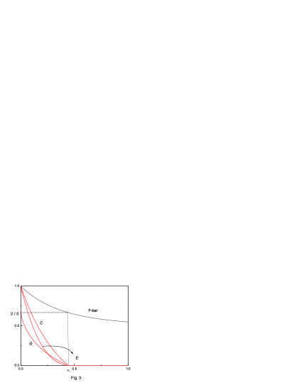
Figure 3: The $\kappa t$-dependence of the average fidelity $\bar{F}$, entanglement of formation ${\cal E}$, concurrence ${\cal C}$ and Groverian measure $G$ for different-axis noisy channels. As expected all entanglement measures reduce to zero when $\kappa t\geq\nu_{*}=\ln(1+\sqrt{2})/2$.

In this section we would like to consider the different-axis noises to confirm that our conjecture is right. First let us consider ($L_{2,x}$, $L_{3,z}$) noise. For this case the master equation (5) changes the EPR state $\rho_{EPR}$ into

$$\varepsilon_{xz}(\rho_{EPR})=\frac{1}{2}\left(\begin{array}[]{cccc}\nu_{+}&0&0&e^{-2\kappa t}\nu_{+}\\ 0&\nu_{-}&e^{-2\kappa t}\nu_{-}&0\\ 0&e^{-2\kappa t}\nu_{-}&\nu_{-}&0\\ e^{-2\kappa t}\nu_{+}&0&0&\nu_{+}\end{array}\right)$$ (52)

where $\nu_{\pm}=(1\pm e^{-2\kappa t})/2$. Following the calculation of Ref.oh02 , one can show easily that the average fidelity in this noise channel becomes

$$\bar{F}=\frac{1}{6}\left(3+2e^{-2\kappa t}+e^{-4\kappa t}\right).$$ (53)

Thus $\bar{F}$ becomes less than $2/3$ when $\kappa t\geq\nu_{*}=\ln(1+\sqrt{2})/2$. We expect that $\varepsilon_{xz}(\rho_{EPR})$ becomes separable in the region $\kappa t\geq\nu_{*}$. In fact, in this region $\varepsilon_{xz}(\rho_{EPR})$ can be expressed as $\varepsilon_{xz}(\rho_{EPR})=\sum_{i=1}^{4}|\bar{s}_{i}\rangle\langle\bar{s}_{i}|$ where $|\bar{s}_{i}\rangle$ are unnormalized vectors defined by same with Eq.(41), but $|x_{i}\rangle$ are

$$|x_{1}\rangle=-i\nu_{+}|e_{1}\rangle\hskip 28.45274pt|x_{2}\rangle=-i\sqrt{\nu_{+}\nu_{-}}|e_{2}\rangle$$ (54)

$$|x_{3}\rangle=-i\sqrt{\nu_{+}\nu_{-}}|e_{3}\rangle\hskip 28.45274pt|x_{4}\rangle=-i\nu_{-}|e_{4}\rangle$$

and $\theta_{i}$’s satisfy

$$e^{2i\theta_{1}}\nu_{+}^{2}+\left(e^{2i\theta_{2}}+e^{2i\theta_{3}}\right)\nu_{+}\nu_{-}+e^{2i\theta_{4}}\nu_{-}^{2}=0.$$ (55)

Since all $|\bar{s}_{i}\rangle$ have zero concurrence, $\varepsilon_{xz}(\rho_{EPR})$ is manifestly separable in $\kappa t\geq\nu_{*}$ as expected.

In the region $\kappa t\leq\nu_{*}$ we can derive an optimal ensemble of pure states. It needs a tedious calculation, and the final expression is $\varepsilon_{xz}(\rho_{EPR})=\sum_{i=1}^{4}P_{i}|XZ_{i}\rangle\langle XZ_{i}|$ where $P_{1}=P_{2}=\nu_{+}/(1+2\nu_{+})$, $P_{3}=P_{4}=1/(2(1+2\nu_{+}))$, and

$$|XZ_{1}\rangle=\nu_{+}|e_{1}\rangle-i\sqrt{\nu_{-}(1+\nu_{+})}|e_{2}\rangle$$ (56)

$$|XZ_{2}\rangle=\nu_{+}|e_{1}\rangle+i\nu_{+}\sqrt{\frac{\nu_{-}}{1+\nu_{+}}}|e_{2}\rangle-i\nu_{+}\sqrt{\frac{\nu_{-}(1+2\nu_{+})}{1+\nu_{+}}}|e_{3}\rangle$$

$$|XZ_{3}\rangle=\nu_{+}|e_{1}\rangle+i\nu_{+}\sqrt{\frac{\nu_{-}}{1+\nu_{+}}}|e_{2}\rangle+i\nu_{+}\sqrt{\frac{\nu_{-}(1+2\nu_{+})}{1+\nu_{+}}}|e_{3}\rangle-i\nu_{-}\sqrt{1+2\nu_{+}}|e_{4}\rangle$$

$$|XZ_{4}\rangle=\nu_{+}|e_{1}\rangle+i\nu_{+}\sqrt{\frac{\nu_{-}}{1+\nu_{+}}}|e_{2}\rangle+i\nu_{+}\sqrt{\frac{\nu_{-}(1+2\nu_{+})}{1+\nu_{+}}}|e_{3}\rangle+i\nu_{-}\sqrt{1+2\nu_{+}}|e_{4}\rangle.$$

Using Eq.(56) it is easy to compute the concurrence whose explicit expression is

$${\cal C}_{xz}=\frac{1}{2}\left(e^{-4\kappa t}+2e^{-2\kappa t}-1\right)$$ (57)

at $\kappa t\leq\nu_{*}$. Thus in the full range of $\kappa t$ ${\cal C}(\rho_{EPR})$ can be written as

$${\cal C}_{xz}=\mbox{Max}\left[\frac{1}{2}\left(e^{-4\kappa t}+2e^{-2\kappa t}-1\right),0\right].$$ (58)

Inserting Eq.(58) into Eq.(33) and Eq.(34), one can compute straightforwardly the entanglement of formation and the Groverian measure for $\varepsilon_{xz}(\rho_{EPR})$.

For ($L_{2,x}$, $L_{3,y}$) and ($L_{2,y}$, $L_{3,z}$) noises the EPR state becomes respectively

$$\varepsilon_{xy}(\rho_{EPR})=\frac{1}{2}\left(\begin{array}[]{cccc}\tau_{+}&0&0&e^{-2\kappa t}\\ 0&\tau_{-}&0&0\\ 0&0&\tau_{-}&0\\ e^{-2\kappa t}&0&0&\tau_{+}\end{array}\right)$$ (63)

$$\varepsilon_{yz}(\rho_{EPR})=\frac{1}{2}\left(\begin{array}[]{cccc}\nu_{+}&0&0&e^{-2\kappa t}\nu_{+}\\ 0&\nu_{-}&e^{-2\kappa t}\nu_{-}&0\\ 0&e^{-2\kappa t}\nu_{-}&\nu_{-}&0\\ e^{-2\kappa t}\nu_{+}&0&0&\nu_{+}\end{array}\right).$$ (68)

It is not difficult to show that the average fidelity for these are equal to Eq.(53) and their concurrences are same with Eq.(58), i.e. concurrence for $\varepsilon_{xz}(\rho_{EPR})$. The optimal ensembles are $\varepsilon_{xy}(\rho_{EPR})=\sum_{i=1}^{4}P_{i}|XY_{i}\rangle\langle XY_{i}|$ and $\varepsilon_{yz}(\rho_{EPR})=\sum_{i=1}^{4}P_{i}|YZ_{i}\rangle\langle YZ_{i}|$, where $P_{1}=P_{2}=\nu_{+}/(1+2\nu_{+})$ and $P_{3}=P_{4}=1/(2(1+2\nu_{+}))$. The optimal pure states $|YZ_{i}\rangle$ can be obtained from $|XZ_{i}\rangle$ by interchanging $|e_{3}\rangle$ and $|e_{4}\rangle$. The optimal vectors $|XY_{i}\rangle$ are obtained from $|XZ_{i}\rangle$ by cyclic change, i.e. $|e_{2}\rangle\rightarrow|e_{3}\rangle$, $|e_{3}\rangle\rightarrow|e_{4}\rangle$, $|e_{4}\rangle\rightarrow|e_{2}\rangle$. The remaining different-axis noises ($L_{2,z}$, $L_{3,x}$), ($L_{2,z}$, $L_{3,y}$), ($L_{2,y}$, $L_{3,x}$) generate similar quantum channels to Eq.(52) and Eq.(63). They also yield same average fidelities and same concurrences.

The average fidelity $\bar{F}$, concurrence ${\cal C}$, entanglement of formation ${\cal E}$ and the Groverian measure $G$ are plotted in Fig. 3. As expected, all entanglement meaures reduce to zero at $\kappa t\geq\nu_{*}$. Thus our conjecture described in section 1 is perfectly correct. This fact indicates that the entanglement of the quantum channel is a genuine physical resource in the teleportation process. Also our conjecture may offer valuable clues for the optimal decomposition in the higher-qubit mixed states. This will be discussed briefly in the next section.

V conclusion

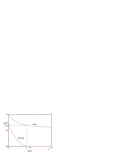
Figure 4: The $\kappa t$-dependence of the average fidelity $\bar{F}$ and Groverian measure $G$ for $3$-qubit mixed state $\varepsilon(\rho_{W})$. The optimal ensemble for $\varepsilon(\rho_{W})$ should make $G$ to be zero when $\kappa t\geq\xi_{*}$. This may give valuable information for the construction of the optimal ensemble for higher-qubit states.

In this paper we have examined the connection between the mixed state entanglement and the average fidelity $\bar{F}$ using usual EPR-state teleportation via noises. As we have shown, the mixed state entanglement becomes zero when $\bar{F}\leq 2/3$, which indicates that the entanglement of quantum channel is a genuine resource for teleportation.

It is generally non-trivial task to compute the entanglement of $n$-qubit mixed states when $n\geq 3$. As far as we know, in addition, there is no way to find an optimal ensemble of pure states when $n\geq 3$. Also we cannnot define the concurrence because there is no “magic”-like basis in higher-qubit system. However, the result of our paper may provide a valuable information on the entanglement of higher-qubit mixed states. For example, let us consider $3$-qubit mixed state

$$\varepsilon(\rho_{W})=\frac{1}{16}\left(\begin{array}[]{cccccccc}2\alpha_{2}&0&0&\sqrt{2}\alpha_{2}&0&\sqrt{2}\alpha_{2}&\alpha_{2}&0\\ 0&2\alpha_{1}&\sqrt{2}\alpha_{1}&0&\sqrt{2}\alpha_{1}&0&0&\alpha_{3}\\ 0&\sqrt{2}\alpha_{1}&2\beta_{+}&0&\alpha_{1}&0&0&\sqrt{2}\alpha_{3}\\ \sqrt{2}\alpha_{2}&0&0&2\beta_{-}&0&\alpha_{4}&\sqrt{2}\alpha_{4}&0\\ 0&\sqrt{2}\alpha_{1}&\alpha_{1}&0&2\beta_{+}&0&0&\sqrt{2}\alpha_{3}\\ \sqrt{2}\alpha_{2}&0&0&\alpha_{4}&0&2\beta_{-}&\sqrt{2}\alpha_{4}&0\\ \alpha_{2}&0&0&\sqrt{2}\alpha_{4}&0&\sqrt{2}\alpha_{4}&2\alpha_{4}&0\\ 0&\alpha_{3}&\sqrt{2}\alpha_{3}&0&\sqrt{2}\alpha_{3}&0&0&2\alpha_{3}\end{array}\right)$$ (77)

where

$$\alpha_{1}=1+e^{-2\kappa t}+e^{-4\kappa t}+e^{-6\kappa t}$$ (78)

$$\alpha_{2}=1+e^{-2\kappa t}-e^{-4\kappa t}-e^{-6\kappa t}$$

$$\alpha_{3}=1-e^{-2\kappa t}-e^{-4\kappa t}+e^{-6\kappa t}$$

$$\alpha_{4}=1-e^{-2\kappa t}+e^{-4\kappa t}-e^{-6\kappa t}$$

$$\beta_{\pm}=1\pm e^{-6\kappa t}.$$

This mixed state is constructed when the quantum teleportation is performed with W-state

$$|\psi_{W}\rangle=\frac{1}{2}\left(|100\rangle+|010\rangle+\sqrt{2}|001\rangle\right)$$ (79)

if ($L_{2,x}$, $L_{3,x}$, $L_{4,x}$) noise is introducedall1 . It has been shown in Ref.all1 that its average fidelity between Alice and Bob is

$$\bar{F}=\frac{1}{24}\left(14+3e^{-2\kappa t}+2e^{-4\kappa t}+5e^{-6\kappa t}\right).$$ (80)

Thus $\bar{F}$ decreases from $1$ to $7/12$ as $\kappa t$ goes from $0$ to $\infty$. From this fact we can conjecture that the Groverian measure (30) for $\varepsilon(\rho_{W})$ decreases from $1/\sqrt{2}$ to $0$ when $\kappa t$ goes from $0$ to $\xi_{*}=0.431041$ if we find the optimal ensemble of pure states for this mixed state. This conjecture is described in Fig. 4. This information may give valuable clues for the construction of the optimal ensemble of pure states in three- or higher-qubit system.

Another point we would like to note is on the second definition of the Groverian measure $\tilde{G}(\rho)$ defined in Eq.(31). Since it is not defined by convex roof construction due to its operational meaning, we cannot use usual optimal ensemble technique to compute it. Since, furthermore, it is expressed as Eq.(32) via Uhlmann’s theorem, we should know how to compute the Groverian measure of $n$-qubit pure states with $n\geq 4$. Even if we assume that we have formula for $n$-qubit pure-state Groverian measure, it is also highly non-trivial to take a maximization over all possible purification. Since, however, it is a genuine entanglement measure for mixed states, it should satisfy our conjecture. It may shed light on the development of the computational technique for $\tilde{G}(\rho)$ in the future.

Acknowledgement: This work was supported by the Kyungnam University Foundation Grant, 2008.

References

(1) M. A. Nielsen and I. L. Chuang, Quantum Computation and
Quantum Information (Cambridge University Press, Cambridge, England, 2000).
(2) G. Vidal, Efficient classical simulation of slightly
entangled quantum computations, Phys. Rev. Lett. 91 (2003)
147902 [quant-ph/0301063].
(3) C. H. Bennett, H. J. Bernstein, S. Popescu and B. Schumacher,
Concentrating partial entanglement by local operation, Phys. Rev. A 53
(1996) 2046 [quant-ph/9511030].
(4) S. Hill and W. K. Wootters, Entanglement of a Pair of Quantum Bits,
Phys. Rev. Lett. 78 (1997) 5022 [quant-ph/9703041].
(5) W. K. Wootters, Entanglement of Formation of an Arbitrary State
of Two Qubits, Phys. Rev. Lett. 80 (1998) 2245 [quant-ph/9709029].
(6) Y. Most, Y. Shimoni and O. Biham, Formation of MultipartiteEntanglement Using Random Quantum Gates, Phys. Rev. A 76
(2007) 022328, arXiv:0708.3481[quant-ph].
(7) O. Biham, M. A. Nielsen and T. J. Osborne, Entanglement
monotone derived from Grover’s algorithm, Phys. Rev. A65 (2002) 062312
[quant-ph/0112097].
(8) L. K. Grover, Quantum Mechanics helps in searching for a needle
in a haystack, Phys. Rev. Lett. 79 (1997) 325 [quant-ph/9706033].
(9) Y. Shimoni, D. Shapira and O. Biham, Characterization of
pure quantum states of multiple qubits using the Groverian entangled measure,
Phys. Rev. A 69 (2004) 062303 [quant-ph/0309062].
(10) L. Tamaryan, DaeKil K. Park and S. Tamaryan,
Analytic Expressions for Geometric Measure of Three Qubit
States, Phys. Rev. A 77 (2008) 022325,
arXiv:0710.0571[quant-ph].
(11) L. Tamaryan, DaeKil Park, Jin-Woo Son, S. Tamaryan, Geometric
Measure of Entanglement and Shared Quantum States,
arXiv:0803.1040 [quant-ph].
(12) E. Jung, Mi-Ra Hwang, DaeKil Park, L. Tamaryan and S. Tamaryan,
Three-Qubit Groverian Measure, arXiv:0803.3311 [quant-ph].
(13) E. Jung, M. R. Hwang, H. Kim, M. S. Kim, D. K. Park, J. W. Son
and S. Tamaryan, Entanglement measures of multiqubit states,
arXiv:0709.4292[quant-ph].
(14) C. H. Bennett, G. Brassard, C. Crépeau, R. Jozsa,
A. Peres and W. K. Wootters, Teleporting an Unknown Quantum State via
Dual Classical and Einstein-Podolsky-Rosen Channles,
Phys. Rev. Lett. 70 (1993) 1895.
(15) S. Oh, S. Lee and H. Lee, Fidelity of quantum teleportation
through noisy channels, Phys. Rev. A66 (2002) 022316 [quant-ph/0206173].
(16) G. Lindbald, On the generators of quantum dynamical
semigroups, Commun. Math. Phys. 48 (1976) 199.
(17) S. Popescu, Bell’s Inequalities versus Teleportation:
What is Nonlocality, Phys. Rev. Lett. 72 (1994) 797.
(18) C. H. Bennett, D. P. DiVincenzo, J. A. Smokin and W. K. Wootters,
Mixed-state entanglement and quantum error correction, Phys. Rev. A54
(1996) 3824 [quant-ph/9604024].
(19) A. Uhlmann, Fidelity and concurrence of conjugate states,
Phys. Rev. A 62 (2000) 032307 [quant-ph/9909060].
(20) G. Vidal, Entanglement monotones, J. Mod. Opt. 47
(2000) 355 [quant-ph/9807077]
(21) D. Shapira, Y. Shimoni and O. Biham, Groverian measure of
entanglement for mixed states, Phys. Rev. A73 (2006) 044301 [quant-ph/0508108].
(22) A. Uhlmann, The transition probability in the state space of a
-algebra, Rep. Math. Phys. 9 (1976) 273.
(23) A. Peres, Separability Criterion for Density Matrices, Phys.
Rev. Lett. 77 (1996) 1413 [quant-ph/9604005].
(24) M. Horodecki, P. Horodecki and R. Horodecki, Separability of mixed
states: necessary and sufficient conditions, Phys. Lett. A 223 (1996) 1
[quant-ph/9605038].
(25) P. Horodecki, Separability criterion and inseparable mixed states
with partial transposition, Phys. Lett. A 232 (1997) 333 [quant-ph/9703004].
(26) Eylee Jung, Mi-Ra Hwang, You-Hwan Ju, Min-Soo Kim, Sahng-Kyoon Yoo,
Hungsoo Kim, DaeKil Park, Jin-Woo Son, S. Tamaryan, and Seong-Keuck Cha, GHZ
versus W: Quantum Teleportation through Noisy Channels, arXiv:0801.1433 [quant-ph].