Free Distance Bounds for Protograph-Based Regular LDPC Convolutional Codes

Abstract

In this paper asymptotic methods are used to form lower bounds on the free distance to constraint length ratio of several ensembles of regular, asymptotically good, protograph-based LDPC convolutional codes. In particular, we show that the free distance to constraint length ratio of the regular LDPC convolutional codes exceeds that of the minimum distance to block length ratio of the corresponding LDPC block codes.

I Introduction

LDPC convolutional codes, the convolutional counterparts of LDPC block codes, were introduced in [1], and they have been shown to have certain advantages compared to LDPC block codes of the same complexity [2, 3]. In this paper, we use ensembles of $(J,K)$ regular tail-biting LDPC convolutional codes derived from a protograph-based ensemble of LDPC block codes to obtain a lower bound on the free distance to constraint length ratio of unterminated, asymptotically good, periodically time-varying regular LDPC convolutional code ensembles, i.e., ensembles that have the property of free distance growing linearly with constraint length.

In the process, we show that the minimum distances of ensembles of tail-biting LDPC convolutional codes (introduced in [4]) approach the free distance of an associated unterminated, periodically time-varying LDPC convolutional code ensemble as the block length of the tail-biting ensemble increases. We show that, for rate $1/2$ protograph-based ensembles with regular degree distributions, the free distance bounds are consistent with those recently derived for more general regular LDPC convolutional code ensembles in [5] and [6]. Further, the relatively low complexity requirements of computing the bound allows us to calculate new free distance bounds that grow linearly with constraint length for values of $J$ and $K$ that have not been previously considered in the literature. We show, for all the ($J$,$K$)-regular ensembles considered, that the free distance to constraint length ratio exceeds the minimum distance to block length ratio of the corresponding block codes.

The paper is structured as follows. In Section II, we briefly introduce LDPC convolutional codes. Section III summarizes the technique proposed by Divsalar to analyze the asymptotic distance growth behavior of protograph-based LDPC block codes [7]. In Section IV, we discuss methods of forming regular convolutional codes from regular protographs. We then describe the construction of tail-biting LDPC convolutional codes as well as corresponding unterminated, periodically time-varying LDPC convolutional codes in Section V. In addition, we show that the free distance of a periodically time-varying LDPC convolutional code is lower bounded by the minimum distance of the block code formed by terminating it as a tail-biting LDPC convolutional code. Finally, in Section VI we present lower bounds on the free distance of ensembles of regular LDPC convolutional codes based on protographs.

II LDPC convolutional codes

We start with a brief definition of a rate $R=b/c$ binary LDPC convolutional code $\mathcal{C}$. (A more detailed description can be found in [1].) A code sequence $\mathbf{v}_{[0,\infty]}$ satisfies the equation

$$\mathbf{v}_{[0,\infty]}\mathbf{H}_{[0,\infty]}^{\mathtt{T}}=\mathbf{0},$$ (1)

where $\mathbf{H}_{[0,\infty]}^{\mathtt{T}}$ is the syndrome former matrix and

$\mathbf{H}_{[0,\infty]}=$
    $\left[\begin{array}[]{cccccc}\mathbf{H}_{0}(0)&&&&\\ \mathbf{H}_{1}(1)&\mathbf{H}_{0}(1)&&&\\ \vdots&\vdots&&\ddots&\\ \mathbf{H}_{m_{\text{s}}}(m_{\text{s}})&\mathbf{H}_{m_{\text{s}}-1}(m_{\text{s}})&\ldots&\mathbf{H}_{0}(m_{\text{s}})&\\ &\mathbf{H}_{m_{\text{s}}}(m_{\text{s}}+1)&\mathbf{H}_{m_{\text{s}}-1}(m_{\text{s}}+1)&\ldots&\mathbf{H}_{0}(m_{\text{s}}+1)\\ &\ddots&\ddots&&\ddots\end{array}\right]$

is the parity-check matrix of the convolutional code $\mathcal{C}$. The submatrices $\mathbf{H}_{i}(t)$, $i=0,1,\cdots,m_{\text{s}}$, $t\geq 0$, are binary $\left(c-b\right)\times c$ submatrices, given by

$$\mathbf{H}_{i}(t)=\left[\begin{array}[]{ccc}h_{i}^{(1,1)}(t)&\cdots&h_{i}^{(1,c)}(t)\\ \vdots&&\vdots\\ h_{i}^{(c-b,1)}(t)&\cdots&h_{i}^{(c-b,c)}(t)\\ \end{array}\right],$$ (2)

that satisfy the following properties:

1. $\mathbf{H}_{i}(t)=\mathbf{0},~{}i<0$ and $i>m_{s},~{}\forall~{}t.$

2. There is a $t$ such that $\mathbf{H}_{m_{\text{s}}}(t)\neq\mathbf{0}.$

3. $\mathbf{H}_{0}(t)\neq\mathbf{0}$ and has full rank $\forall\,\,t$.

We call $m_{\text{s}}$ the syndrome former memory and $\nu_{\text{s}}=(m_{\text{s}}+1)\cdot c$ the decoding constraint length. These parameters determine the width of the nonzero diagonal region of $\mathbf{H}_{[0,\infty]}.$ The sparsity of the parity-check matrix is ensured by demanding that its rows have very low Hamming weight, i.e., $w_{H}(\mathbf{h}_{i})<<(m_{\text{s}}+1)\cdot c,~{}i>0$, where $\mathbf{h}_{i}$ denotes the $i$-th row of $\mathbf{H}_{[0,\infty]}$. The code is said to be regular if its parity-check matrix $\mathbf{H}_{[0,\infty]}$ has exactly $J$ ones in every column and, starting from row $(c-b)m_{\text{s}}+1$, $K$ ones in every row. The other entries are zeros. We refer to a code with these properties as an $(m_{\text{s}},J,K)$-regular LDPC convolutional code, and we note that, in general, the code is time-varying and has rate $R=1-J/K$. A rate $R=b/c$, $(m_{\text{s}},J,K)$-regular time-varying LDPC convolutional code is periodic with period $cT$ if $\mathbf{H}_{i}(t)$ is periodic, i.e., $\mathbf{H}_{i}(t)=\mathbf{H}_{i}(t+T),\forall~{}i,t$, and if $\mathbf{H}_{i}(t)=\mathbf{H}_{i},\forall~{}i,t$, the code is time-invariant.

III Protograph Weight Enumerators

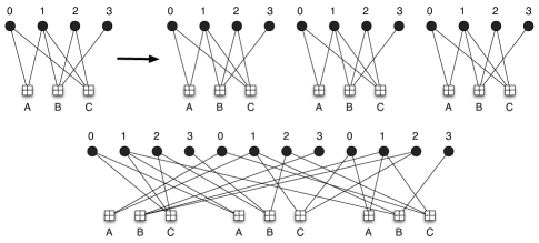
Suppose a given protograph has $n_{v}$ variable nodes and $n_{c}$ check nodes. An ensemble of protograph-based LDPC block codes can be created using the copy-and-permute operation [8]. The Tanner graph obtained for one member of an ensemble created with this method is illustrated in Fig. 1.

Figure 1: The copy-and-permute operation for a protograph.

The parity-check matrix $H$ corresponding to the ensemble of protograph-based LDPC block codes can be obtained by replacing ones with $N\times N$ permutation matrices and zeros with $N\times N$ all zero matrices in the underlying protograph parity-check matrix $P$, where the permutation matrices are chosen randomly and independently. The protograph parity-check matrix $P$ corresponding to the protograph given in Figure 1 can be written as

,

where we note that, since the row and column weights of $P$ are not constant, $P$ represents the parity-check matrix of an irregular LDPC code. For a $(J,K)$ regular LDPC code, the protograph contains $n_{c}=J$ check nodes and $n_{v}=K$ variable nodes, where each variable node is connected to all $J$ check nodes, i.e., $P$ is an “all-one” matrix. The sparsity condition of an LDPC parity-check matrix is thus satisfied for large $N$. The code created by applying the copy-and-permute operation to an $n_{c}\times n_{v}$ protograph parity-check matrix $P$ has block length $n=Nn_{v}$. In addition, the code has the same rate and degree distribution for each of its variable and check nodes as the underlying protograph code.

Combinatorial methods of calculating ensemble average weight enumerators have been presented in [7] and [9]. We now briefly describe the methods presented in [7].

III-A Ensemble weight enumerators

Suppose a protograph contains $m$ variable nodes to be transmitted over the channel and $n_{v}-m$ punctured variable nodes. Also, suppose that each of the $m$ transmitted variable nodes has an associated weight $d_{i}\in\{0,1\}$. Let $S_{d}=\{(d_{1},d_{2},\ldots,d_{m})\}$ be the set of all possible weight distributions such that $d_{1}+\ldots+d_{m}=d$, and let $S_{p}$ be the set of all possible weight distributions for the remaining punctured nodes. The ensemble weight enumerator for the protograph is then given by

$$A_{d}=\sum_{\{d_{k}\}\in S_{d}}\sum_{\{d_{j}\}\in S_{p}}A_{\mathbf{d}},$$ (3)

where $A_{\mathbf{d}}$ is the average number of codewords in the ensemble with a particular weight distribution $\textbf{d}=(d_{1},d_{2},\ldots,d_{n_{v}})$.

III-B Asymptotic weight enumerators

The normalized logarithmic asymptotic weight distribution of a code ensemble can be written as $r(\delta)=\lim_{n\rightarrow\infty}\textrm{sup }r_{n}(\delta),$ where $r_{n}(\delta)=\frac{\textrm{ln}(A_{d})}{n}$, $\delta=d/n$, $d$ is the Hamming weight, $n$ is the block length, and $A_{d}$ is the ensemble average weight distribution.

Suppose the first zero crossing of $r(\delta)$ occurs at $\delta=\delta_{min}$. If $r(\delta)$ is negative in the range $0<\delta<\delta_{min}$, then $\delta_{min}$ is called the minimum distance growth rate of the code ensemble. By considering the probability

$$\mathbb{P}(d<\delta_{min}n)=\sum^{\delta_{min}n-1}_{d=1}A_{d},$$

it is clear that, as the block length $n$ grows, if $\mathbb{P}(d<\delta_{min}n)<<1$, then we can say with high probability that the majority of codes in the ensemble have a minimum distance that grows linearly with $n$ and that the distance growth rate is $\delta_{min}$.

IV Forming Convolutional Codes from Protographs

In this section, we present methods to form convolutional parity-check matrices from the parity-check matrix of a protograph.

IV-A Unwrapping a protograph with gcd$(n_{c},n_{v})>1$

Suppose that we have an $n_{c}\times n_{v}$ protograph parity-check matrix $P$, where gcd$(n_{c},n_{v})=y>1$. We then partition $P$ as a $y\times y$ block matrix as follows:

$$P=\left[\begin{array}[]{ccc}P_{1,1}&\ldots&P_{1,y}\\ \vdots&&\vdots\\ P_{y,1}&\ldots&P_{y,y}\end{array}\right],$$

where each block $P_{i,j}$ is of size $n_{c}/y\times n_{v}/y$. $P$ can now be separated into a lower triangular part, $P_{l}$, and an upper triangular part minus the leading diagonal, $P_{u}$. Explicitly,

$$P_{l}=\left[\begin{array}[]{cccc}P_{1,1}&&\\ P_{2,1}&P_{2,2}&&\\ \vdots&\vdots&\ddots&\\ P_{y,1}&P_{y,2}&\ldots&P_{y,y}\end{array}\right]$$

and

$$P_{u}=\left[\begin{array}[]{cccc}&P_{1,2}&\ldots&P_{1,y}\\ &&\ddots&\vdots\\ &&&P_{y-1,y}\\ &&&\end{array}\right],$$

where blank spaces correspond to zeros. This operation is called ‘cutting’ a protograph parity-check matrix.

Rearranging the positions of these two triangular matrices and repeating them indefinitely results in a parity-check matrix $H_{cc}$ of an unterminated, periodically time-varying convolutional code with decoding constraint length $\nu_{\text{s}}=n_{v}$ and period $T=n_{v}$ given by

$$H_{\textrm{cc}}=\left[\begin{array}[]{cccc}P_{l}&&&\\ P_{u}&P_{l}&&\\ &P_{u}&P_{l}&\\ &&\ddots&\ddots\end{array}\right].$$ (4)

Note that the unwrapping procedure described above preserves the row and column weights of the protograph parity-check matrix.

IV-B Unwrapping a protograph with gcd$(n_{c},n_{v})=1$

If gcd$(n_{c},n_{v})=1$, we cannot form a square block matrix larger than $1\times 1$ with equal size blocks. In this case, $P_{l}=P$ and $P_{u}$ is the all zero matrix of size $n_{c}\times n_{v}$. This trivial cut results in a convolutional code with syndrome former memory zero, with repeating blocks of the original protograph on the leading diagonal. We now propose two methods of dealing with this structure.

IV-B1 Form an $M$-cover

Here, we create a larger protograph parity-check matrix by using the copy and permute operation on $P$. This results in an $Mn_{c}\times Mn_{v}=n_{c}^{\prime}\times n_{v}^{\prime}$ parity-check matrix for some small integer $M$. The $n_{c}^{\prime}\times n_{v}^{\prime}$ protograph parity-check matrix can then be cut following the procedure outlined above. In effect, the $M\times M$ permutation matrix creates a mini ensemble of block codes that can be be unwrapped to an ensemble of convolutional codes. The resulting unterminated, periodically time-varying convolutional code has decoding constraint length $\nu_{\text{s}}=Mn_{v}$ and period $T=Mn_{v}$.

IV-B2 Use a nonuniform cut

When gcd$(n_{c},n_{v})=1$, we can still form a convolutional code by unwrapping the protograph parity-check matrix using a nonuniform cut. Let the protograph parity-check matrix be written as

$$P=\left[\begin{array}[]{cccc}p_{1,1}&\ldots&p_{1,n_{v}}\\ \vdots&&\vdots\\ p_{n_{c},1}&\ldots&p_{n_{c},n_{v}}\end{array}\right].$$

We define a vector $\mathbf{\xi}$ consisting of $n_{c}$ step parameters $\mathbf{\xi}=(\xi_{1},\xi_{2},\ldots,\xi_{n_{c}})$, where $0\leq\xi_{1}<\xi_{n_{c}}\leq n_{v}$, and each $\xi_{i-1}<\xi_{i}$ for $i=2,\ldots,n_{c}$ . As in the previous case, we form $n_{c}\times n_{v}$ matrices $P_{l}$ and $P_{u}$ as follows

• for each $\xi_{i}$, $i=1,\ldots,n_{c}$, the entries $p_{i,1}$ to $p_{i,\xi_{i}}$ are copied into the equivalent positions in $P_{l}$;

• entries $p_{i,\xi_{i}+1}$ to $p_{i,n_{v}}$ are copied, if they exist, into the equivalent positions in $P_{u}$;

• the remaining positions in $P_{l}$ and $P_{u}$ are set to zero.

We now form the parity-check matrix $H_{cc}$ of an unterminated, periodically time-varying convolutional code as in (4). Nonuniform cuts do not change the row and column weights of the parity-check matrix $P$. Further, the decoding constraint length remains constant.

An LDPC convolutional code derived from an LDPC block code using a nonuniform cut can be encoded and decoded using conventional encoding and decoding methods with minor modifications. For an LDPC convolutional code obtained using the nonuniform cut $\xi=(\xi_{1},\ldots,\xi_{n_{c}})$, the maximum step width $\xi_{max}$ for the cut is given by

$$\xi_{max}=\max\limits_{i=2,\ldots,n_{c}}\{\xi_{1},\xi_{i}-\xi_{i-1}\}.$$

$\xi_{max}-\xi_{i}$ columns of zeros are then appended immediately to the left of the columns in the original protograph parity-check matrix $P$ corresponding to the steps $\xi_{i}$, $i=1,2,\ldots,n_{c}$, to form a modified protograph parity-check matrix $P^{\prime}$. This process is demonstrated for a (3,4)-regular protograph with the nonuniform cut $\xi=(2,3,4)$ below:

.

LDPC convolutional codes unwrapped from $P^{\prime}$ can be encoded by a conventional LDPC convolutional encoder with the condition that information symbols are not assigned to the all-zero columns. Thus, these columns correspond to punctured symbols, and the code rate is not affected. At the decoder, a conventional pipeline decoder can be employed to decode the received sequence. No special treatment is necessary for the symbols corresponding to the all-zero columns, since the column weight of zero insures that they are not included in any parity-check equations, i.e., the belief-propagation decoding algorithm ignores the corresponding symbols.

V Free distance bounds

We now introduce the notion of tail-biting convolutional codes by defining an ‘unwrapping factor’ $\lambda$ as the number of times the sliding convolutional structure is repeated. For $\lambda>1$, the parity-check matrix $H_{\textrm{tb}}^{(\lambda)}$ of the desired tail-biting convolutional code can be written as

$$H_{\textrm{tb}}^{(\lambda)}=\left[\begin{array}[]{ccccc}P_{l}&&&&P_{u}\\ P_{u}&P_{l}&&&\\ &P_{u}&P_{l}&&\\ &&\ddots&\ddots&\\ &&&P_{u}&P_{l}\end{array}\right]_{\lambda n_{c}\times\lambda n_{v}}.$$

Note that the tail-biting convolutional code for $\lambda=1$ is simply the original block code.

V-A A tail-biting LDPC convolutional code ensemble

Given a protograph parity-check matrix $P$, we generate a family of tail-biting convolutional codes with increasing block lengths $\lambda n_{v}$, $\lambda=1,2,\ldots$, using the process described above. Since tail-biting convolutional codes are themselves block codes, we can treat the Tanner graph of $H_{\textrm{tb}}^{(\lambda)}$ as a protograph for each value of $\lambda$. Replacing the entries of this matrix with either $N\times N$ permutation matrices or $N\times N$ all zero matrices, as discussed in Section III, creates an ensemble of LDPC codes with block length $n=\lambda Nn_{v}$ that can be analyzed asymptotically as $N$ goes to infinity, where the sparsity condition of an LDPC code is satisfied for large $N$. Each tail-biting LDPC code ensemble, in turn, can be unwrapped and repeated indefinitely to form an ensemble of unterminated, periodically time-varying LDPC convolutional codes with decoding constraint length $\nu_{s}=Nn_{v}$ and period $T=\lambda Nn_{v}$.

Intuitively, as $\lambda$ increases, the tail-biting code becomes a better representation of the associated unterminated convolutional code, with $\lambda\rightarrow\infty$ corresponding to the unterminated convolutional code itself. This is reflected in the weight enumerators, and it is shown in Section VI that increasing $\lambda$ provides us with distance growth rates that converge to a lower bound on the free distance growth rate of the unterminated convolutional code.

V-B A free distance bound

Tail-biting convolutional codes can be used to establish a lower bound on the free distance of an associated unterminated, periodically time-varying convolutional code by showing that the free distance of the unterminated code is lower bounded by the minimum distance of any of its tail-biting versions.

Theorem 1

Consider a rate $R=(n_{v}-n_{c})/n_{v}$ unterminated, periodically time-varying convolutional code with decoding constraint length $\nu_{\text{s}}=Nn_{v}$ and period $T=\lambda Nn_{v}$. Let $d_{min}$ be the minimum distance of the associated tail-biting convolutional code with length $n=\lambda Nn_{v}$ and unwrapping factor $\lambda>0$. Then the free distance $d_{free}$ of the unterminated convolutional code is lower bounded by $d_{min}$ for any unwrapping factor $\lambda$, i.e.,

$$d_{free}\geq d_{min},\quad\forall\lambda>0.$$ (5)

Sketch of proof. It can be shown that any codeword in a rate $R=(n_{v}-n_{c})/n_{v}$ unterminated, periodically time-varying convolutional code with constraint length $\nu_{\text{s}}=Nn_{v}$ and period $T=\lambda Nn_{v}$ can be wrapped back to a codeword in a tail-biting convolutional code of length $n=\lambda Nn_{v}$, for any $\lambda$. The ‘wrapping back’ procedure consists of dividing the convolutional codeword into segments of length $\lambda Nn_{v}$ and superimposing these segments through a modulo summation. The Hamming weight of the resulting codeword in the tail-biting code must be equal to or less than that of the codeword in the unterminated code. The result is then obtained by wrapping back the unterminated codeword with minimum Hamming weight. For a formal proof, see [6].

A trivial corollary of the above theorem is that the minimum distance of a protograph-based LDPC block code is a lower bound on the free distance of the associated unterminated, periodically time-varying LDPC convolutional code. This can be observed by setting $\lambda=1$.

V-C The free distance growth rate

The distance growth rate $\delta_{min}$ of a block code ensemble is defined as its minimum distance to block length ratio. For the protograph-based tail-biting LDPC convolutional codes defined in Section V-A, this ratio is therefore given as

$$\delta_{min}=\frac{d_{min}}{n}=\frac{d_{min}}{\lambda Nn_{v}}=\frac{d_{min}}{\lambda\nu_{\text{s}}}.$$ (6)

Using (5) we obtain

$$\delta_{min}\leq\frac{d_{free}}{\lambda\nu_{\text{s}}},$$ (7)

where $d_{free}$ is the free distance of the associated unterminated, periodically time-varying LDPC convolutional code. It is important to note that, for convolutional codes, the length of the shortest codeword is equal to the encoding constraint length $\nu_{\text{e}}$, which in general differs from the decoding constraint length $\nu_{\text{s}}$. Assuming minimal encoder and syndrome former matrices, the relation between $\nu_{\text{e}}$ and $\nu_{\text{s}}$ can be expressed as

$$\nu_{\text{e}}=\frac{1-R}{R}\nu_{\text{s}},$$ (8)

which implies that, for code rates less than $1/2$, the encoding constraint length is larger than the decoding constraint length.

Combining (7) and (8) gives us the desired bound on the free distance growth rate

$$\delta_{free}\geq\frac{R}{1-R}\lambda\delta_{min},$$ (9)

where $\delta_{free}=d_{free}/\nu_{e}$ is the convolutional code free distance growth rate.

VI Bound computations

We now present free distance growth rate results for ensembles of asymptotically good, regular, LDPC convolutional codes based on protographs. We consider all the regular ensembles originally considered by Gallager [10], and for each we calculate a lower bound on the free distance to constraint length ratio $\delta_{free}$. We begin by considering the regular ensembles with gcd$(n_{c},n_{v})>1$. Then we consider the methods proposed in Section IV-B for regular ensembles with gcd$(n_{c},n_{v})=1$. Results for these ensembles are then presented and discussed.

VI-A Regular Ensembles with gcd$(n_{c},n_{v})>1$

Example $1$: Consider the rate $R=1/2$, $(3,6)$-regular LDPC code ensemble based on the following protograph:

.

For this example, the minimum distance growth rate is $\delta_{min}=0.023$, as originally computed by Gallager [10]. A family of tail-biting $(3,6)$-regular LDPC convolutional code ensembles can be generated according to the following cut:

.

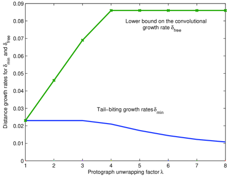
For $\lambda=2,3,\ldots,8$, the minimum distance growth rate $\delta_{min}$ was calculated for the tail-biting LDPC convolutional code ensembles using the approach outlined in Section V-A. These growth rates are shown in Fig. 2, along with the corresponding lower bound on the free distance growth rate $\delta_{free}$ of the associated ensemble of unterminated, periodically time-varying LDPC convolutional codes. For this rate $R=1/2$ ensemble, the lower bound on $\delta_{free}$ is simply $\delta_{free}\geq\frac{R}{1-R}\lambda\delta_{min}=\lambda\delta_{min}$, since $\frac{R}{1-R}=1$ in this case.

Figure 2: Distance growth rates for Example $1$.

We observe that, once the unwrapping factor $\lambda$ of the tail-biting convolutional codes exceeds $3$, the lower bound on $\delta_{free}$ levels off at $\delta_{free}\geq 0.086$, which agrees with the results presented in [5] and [6] and represents a significant increase over the value of $\delta_{min}$. In this case, the minimum weight codeword in the unterminated convolutional code also appears as a codeword in the tail-biting code.

Example $2$: Consider the rate $R=1/3$, $(4,6)$-regular LDPC code ensemble. The minimum distance growth rate for this ensemble is $\delta_{min}=0.128$ [10]. We form a protograph in the usual fashion, creating $4$ check nodes, each of which connect to all $6$ variable nodes, and we observe that gcd$(4,6)=2$. The protograph parity-check matrix and defined cut are displayed below:

.

For this rate $R=1/3$ ensemble, the lower bound on $\delta_{free}$ is $\delta_{free}\geq\frac{R}{1-R}\lambda\delta_{min}=\frac{1}{2}\lambda\delta_{min}$. We observe that, as in Example $1$, the minimum distance growth rates calculated for increasing $\lambda$ provide us with a lower bound $\delta_{free}\geq 0.197$ on the free distance growth rate of the convolutional code ensemble, which exceeds the value of $\delta_{min}$.

Example $3$: Consider the rate $R=1/2$, $(4,8)$-regular LDPC code ensemble. The minimum distance growth rate for this ensemble is $\delta_{min}=0.063$ [10]. The protograph parity-check matrix is cut along the diagonal in steps of $1\times 2$. For this rate $R=1/2$ ensemble, the lower bound on $\delta_{free}$ is $\delta_{free}\geq\frac{R}{1-R}\lambda\delta_{min}=\lambda\delta_{min}$, and we obtain the lower bound $\delta_{free}\geq 0.191$ on the free distance growth rate of the convolutional code ensemble, which is again significantly larger than $\delta_{min}$.

VI-B Regular Ensembles with gcd$(n_{c},n_{v})=1$

We now present results for the two methods of unwrapping a protograph with gcd$(n_{c},n_{v})=1$ introduced in Section IV-B.

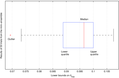
Example $4$: Consider the rate $R=2/5$, $(3,5)$-regular ensemble. The minimum distance growth rate for this ensemble is $\delta_{min}=0.045$ [10]. For this rate $R=2/5$ ensemble, the lower bound on $\delta_{free}$ is $\delta_{free}\geq\frac{R}{1-R}\lambda\delta_{min}=\frac{2}{3}\lambda\delta_{min}$. The first approach was to form a two-cover of the regular protograph. The resulting mini-ensemble has $2^{n_{v}n_{c}}=2^{15}$ members. Fifty distinct members were chosen randomly. The resulting lower bounds calculated for $\delta_{free}$ are shown in a box plot in Fig. 3.

Figure 3: Free distance growth rates for $50$ mini-ensemble members.

We observe a fairly large spread in results from the mini-ensemble. The median from the fifty trials is $\delta_{free}=0.097$. We also observe that the smallest lower bound found is statistically a outlier as it lies reasonably far away from the lower quartile. Note that this smallest lower bound ($\delta_{free}\geq 0.069$) is larger than the block code growth rate $\delta_{min}=0.045$. Also, the best lower bound, $\delta_{free}\geq 0.108$, is significantly larger than $\delta_{min}$.

We now consider the nonuniform cut case. Consider the following two nonuniform cuts of the standard protograph parity-check matrix for the regular $(3,5)$ ensemble:

and ,

with corresponding cutting vectors $\xi_{1}=(2,4,5)$ and $\xi_{2}=(1,2,3)$. We calculate a lower bound of $\delta_{free}\geq 0.119$ for cut one and $\delta_{free}\geq 0.111$ for cut two. Both nonuniform cuts give larger lower bounds on $\delta_{free}$ than the mini-ensemble method.

For the remaining regular ensembles with gcd$(n_{c},n_{v})=1$, we used the nonuniform cut method. The resulting bounds are given in the table below.

Ensemble	Cut $\mathbf{\xi}$	$\delta_{min}$ [10]	Lower bound on $\delta_{free}$
$(3,4)$	$(2,3,4)$	$0.112$	$0.177$
$(4,5)$	$(2,3,4,5)$	$0.210$	$0.266$
$(5,6)$	$(2,3,4,5,6)$	$0.254$	$0.317$

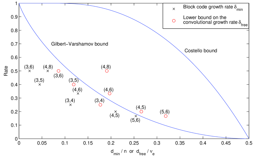
For each ensemble considered, the lower bound on $\delta_{free}$ is significantly larger than $\delta_{min}$ for the block code ensemble. This is illustrated in Fig. 4, where the distance growth rates of each regular LDPC code ensemble are compared to the corresponding bounds for general block and convolutional codes.

Figure 4: Comparison of calculated growth rates with the Gilbert-Varshamov bound for block code minimum distance growth rates and the Costello bound for convolutional code free distance growth rates.

VII Conclusions

In this paper, asymptotic methods were used to calculate a lower bound on free distance that grows linearly with constraint length for several ensembles of regular, unterminated, protograph-based periodically time-varying LDPC convolutional codes. It was shown that the free distance growth rates of the regular LDPC convolutional code ensembles exceed the minimum distance growth rates of the corresponding regular LDPC block code ensembles. When gcd$(n_{c},n_{v})=1$, we proposed two new methods of unwrapping the protograph parity-check matrix in order to obtain the best possible lower bound on $\delta_{free}$. The results suggest that we typically obtain better lower bounds by performing nonuniform cuts.

References

- [1] A. Jiménez Felström and K. Sh. Zigangirov, “Time-varying periodic convolutional codes with low-density parity-check matrices”, IEEE Trans. Inform. Theory, IT-45, pp.2181-2191, Sept. 1999.
- [2] D. J. Costello, Jr., A. E. Pusane, S. Bates, and K. Sh. Zigangirov, “A comparison between LDPC block and convolutional codes”, Proc. Information Theory and Applications Workshop, San Diego, CA, USA, Feb. 2006.
- [3] D. J. Costello, Jr., A. E. Pusane, C. R. Jones, and D. Divsalar, “A comparison of ARA- and protograph-based LDPC block and convolutional codes”, Proc. Information Theory and Applications Workshop, San Diego, CA, USA, Feb. 2007.
- [4] M. Tavares, K. Sh. Zigangirov, and G. Fettweis, “Tail-Biting LDPC Convolutional Codes”, Proc. IEEE International Symposium on Information Theory, Nice, France, June 2007.
- [5] A. Sridharan, D. Truhachev, M. Lentmaier, D. J. Costello, Jr., and K. Sh. Zigangirov, “Distance bounds for an ensemble of LDPC convolutional codes”, IEEE Trans. Inform. Theory, IT-53, pp. 4537-4555, Dec. 2007.
- [6] D. Truhachev, K. Sh. Zigangirov, and D. J. Costello, Jr., “Distance bounds for periodic LDPC convolutional codes and tail-biting convolutional codes”, IEEE Trans. Inform. Theory (submitted), Jan. 2008.
- [7] D. Divsalar, “Ensemble Weight Enumerators for Protograph LDPC Codes”, Proc. IEEE International Symposium on Information Theory, Seattle, WA, Jul. 2006.
- [8] J. Thorpe, “Low-Density Parity-Check (LDPC) codes constructed from protographs”, JPL INP Progress Report, Vol. 42-154, Aug. 2003.
- [9] S. L. Fogal, R. McEliece, and J. Thorpe, “Enumerators for protograph ensembles of LDPC codes”, Proc. IEEE International Symposium on Information Theory, Adelaide, Australia, Sept. 2005.
- [10] R. G. Gallager, “Low-density parity-check codes”, IRE Trans. Inform. Theory, IT-8: 21-28, Jan. 1962.
- [11] D. G. M. Mitchell, A. E. Pusane, K. Sh. Zigangirov, and D. J. Costello, Jr. , “Asymptotically Good LDPC Convolutional Codes Based on Protographs”, 2008 IEEE International Symposium on Information Theory (accepted).