Magnetic moments of long isotopic chains

Abstract

Dipole magnetic moments of several long isotopic chains are analyzed within the self-consistent Finite Fermi System theory based on the Generalized Energy Density Functional method with exact account for the pairing and quasi-particle continuum. New data for nuclei far from the $\beta$-stability valley are included in the analysis. For a number of semi-magic isotopes of the tin and lead chains a good description of the data is obtained, with accuracy of $0.1{-}0.2\mu_{\rm N}$. A chain of non-magic isotopes of copper is also analyzed in detail. It is found that the systematic analysis of magnetic moments of this long chain yields rich information on the evolution of the nuclear structure of the Cu isotopes. In particular, it may give a signal of deformation for the ground state of some nuclei in the chain.

I Introduction

Dipole magnetic moments of atomic nuclei are one of the fundamental nuclear characteristics. Their interpretation played an important role in the formulation of basic theoretical approaches in nuclear physics, such as the Shell Model (SM) Bohr and the Finite Fermi System (FFS) theory AB1 . Modern RIB facilities provide an access to long chains of isotopes including the radioactive ones in their ground and isomeric states. Spectroscopy techniques using high intensity lasers allow for precision measurements of nuclear spins and magnetic moments. As a result, the bulk of the data on nuclear magnetic moments becomes very extensive and comprehensive Stone creating a challenge to nuclear theory.

Recently, the self-consistent version of the FFS theory was applied to describe magnetic moments of more than 100 odd-A spherical heavy and intermediate atomic mass nuclei BST . This approach is based on the so-called Generalized Energy Density Functional (EDF) method for nuclei with pairing correlations STF ; Fay . It involves explicit consideration of the pion and $\rho$-meson degrees of freedom and the method of finding the FFS (RPA-like) response function with exact account for all continuum states. The latter was developed in ShB ; SapTF for magic nuclei and in Plat for the general case taking into account pairing correlations. With the exception of a number of cases, a high precision description with accuracy of $0.1{-}0.2\mu_{\rm N}$ was obtained in BST . In these calculations the “one-quasiparticle” approximation was used in which an odd nucleus is considered as a system with a quasiparticle added to the even-even core in the state $\lambda_{0}$ at the Fermi surface. In the FFS theory, the quasiparticle differs from the particle in the SM in two respects. First, it possesses the effective local quasiparticle charge $e_{q}[V_{0}]$ for the external field $V_{0}$ under consideration. This charge is, as a rule, different from that of the bare particle. Second, the core is polarized with the quasiparticle, via the so-called Landau–Migdal interaction amplitude ${\cal F}$, playing the role of the effective interaction in the FFS theory. In this approach, both effects are taken into account in the equation for the effective field $V$ in terms of the bare field $V_{0}$, $e_{q}[V_{0}]$ and ${\cal F}$, the magnetic moment value being given by the single-particle matrix element $\mu_{\lambda_{0}}=(V[\hat{\boldsymbol{\mu}}])_{\lambda_{0}\lambda_{0}}$. It should be noted that in BST , in addition to the two standard FFS theory local charges with respect to the magnetic field, i.e. the spin $\zeta_{s}$ and orbit $\zeta_{l}$ local charges, a new, tensor local charge $\zeta_{t}$ was added. It is defined in such a way that the corresponding contribution to the magnetic moment operator is $\delta\mu_{t}=\zeta_{t}\sqrt{4\pi}\,[{\bf Y}_{2}({\bf n})\circledast\hat{\boldsymbol{\sigma}}]^{1}_{\mu}\,\hat{\tau}_{3}$, where ${\bf n}={\bf r}/r$, and $\hat{\tau}_{3}$ is the third isospin Pauli matrix. It turned out that introducing such local charge with $\zeta_{t}=0.2$ makes the overall agreement of the theory with experiment better, especially for nuclei with the odd nucleon in the state $\lambda_{0}=p_{1/2}$. Other FFS theory parameters entering the calculation scheme in the case of the magnetic symmetry were taken from PF ; BorTF .

In this paper, within the same approach as in BST , we concentrate on the analysis of magnetic moments of long isotopic chains. Recently a lot of experimental data have been obtained for Cu isotopes Minam ; Isolde_Cu ; Cu_1 and Pb-isotopes Pb . We have analyzed the cases for which a simple approach BST based on the assumption of sphericity and on the one-quasiparticle approximation is not compatible with data. It was found that in several cases the contribution of more complicated configurations should be taken into account. Further, for nuclei at the extremes of the isotopic chains the deformation was found to play a role as well.

II Semi-magic nuclei

Let us begin from the analysis of the global behavior of magnetic moments for the two chains of semi-magic isotopes of tin ($Z=50$) and lead ($Z=82$). Ground state energies and radii of both isotopic chains were analyzed in detail by S.A. Fayans et al. Fay within the Generalized EDF method STF which is a generalization to superfluid systems of the well-known EDF method by Kohn and Sham KS developed originally for normal Fermi systems. The Sn and Pb chains were analyzed assuming a spherical shape for the ground state. The very good description of masses and radii, including the odd-even effects, confirmed this assumption. This is in agreement with the systematic analysis of nuclear deformations carried out in HF within the Advanced Thomas-Fermi method with the Shell-Model correction of V.M. Strutinsky. It should be noted that we use the term “spherical” for odd nuclei neglecting a small ($\propto 1/A$) deformation effect of the odd nucleon. In fact, this is taken into account in the FFS theory equations for the effective field $V$ by calculating the core polarization induced by this particle.

We start with the Sn chain containing 12 odd isotopes, from ¹⁰⁹Sn to ¹³¹Sn, with neutron number varying from $N_{\rm min}=59$ to $N_{\rm max}=81$. Note that we consider only nuclei with known experimental values of the magnetic moment in the ground or excited state. Among these nuclei, only ^115-119Sn are stable, i.e. the $\beta$-stability valley for odd Sn isotopes has boundaries at $N^{\beta}_{\rm min}=65$ and $N^{\beta}_{\rm max}=69$. Thus, the maximum neutron excess is $\delta N_{+}=N_{\rm max}-N^{\beta}_{\rm max}=12$ and the deficiency, $\delta N_{-}=N^{\beta}_{\rm min}-N_{\rm min}=6$. It is instructive to consider also the relative maximum neutron excess, $\varepsilon_{+}=\delta N_{+}/N^{\beta}_{\rm max}=17.4\%$, and deficiency, $\varepsilon_{-}=\delta N_{-}/N^{\beta}_{\rm min}=9.2\%$.

A comparison of 25 theoretical values of magnetic moments with the corresponding experimental data taken from Stone is given in Table I and Fig. 1. For convenience, we present also the difference $\delta\mu=\mu_{\rm th}-\mu_{\rm exp}$ which characterizes directly the global accuracy of the theory. As we see, this accuracy is sufficiently high: as a rule, we obtained $|\delta\mu|<0.1\mu_{\rm N}$, and only in four cases $0.1\mu_{\rm N}<|\delta\mu|<0.15\mu_{\rm N}$. Except for two out of 25 cases (i.e. ¹¹³Sn and ¹¹⁵Sn) all experimental magnetic moments are reproduced within 10%.

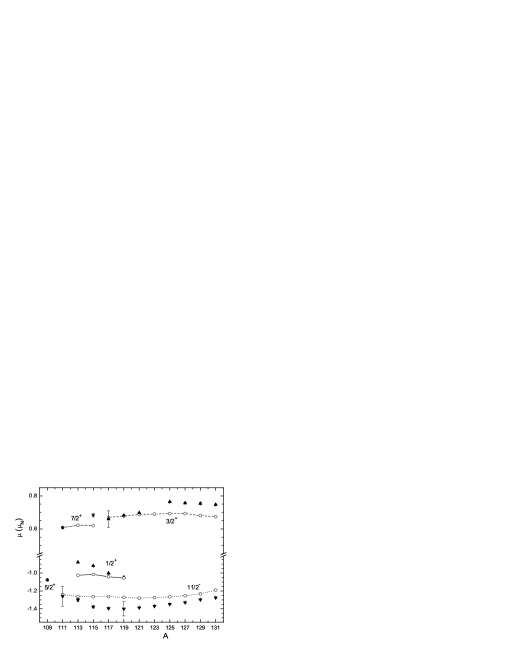
Figure 1: Magnetic moments of Sn isotopes. The experimental data are shown with filled triangles (up and down) Stone . Open circles show the theoretical predictions. The quantum numbers of the single-particle configurations assumed in our calculations are also indicated.

Table 1: Magnetic moments (in $\mu_{\rm N}$) of Sn isotopes. The experimental data are from Stone . The symbol * indicates excited states.

nucleus	neutron s.p. state $\lambda_{0}^{n}$	$\mu_{\rm exp}$	$\mu_{\rm Sch}$	$\mu_{\rm th}$	$\delta\mu$
${}^{109}{\rm Sn}$	$d_{5/2}$	-1.079(6)	-1.913	-1.074	0.005(6)
${}^{111}{\rm Sn}$	$g_{7/2}$	0.608(4)	1.488	0.608	0.000(4)
${}^{115}{\rm Sn}^{*}$	$g_{7/2}$	0.683(10)	1.488	0.620	-0.06(1)
${}^{113}{\rm Sn}$	$s_{1/2}$	-0.8791(6)	-1.913	-1.025	-0.146
${}^{115}{\rm Sn}$	$s_{1/2}$	-0.91883(7)	-1.913	-1.015	-0.096
${}^{117}{\rm Sn}$	$s_{1/2}$	-1.00104(7)	-1.913	-1.042	-0.041
${}^{119}{\rm Sn}$	$s_{1/2}$	-1.04728(7)	-1.913	-1.056	-0.009
${}^{111}{\rm Sn}^{*}$	$h_{11/2}$	-1.26(11)	-1.913	-1.240	0.02(11)
${}^{113}{\rm Sn}^{*}$	$h_{11/2}$	-1.30(2)	-1.913	-1.262	0.04(2)
${}^{115}{\rm Sn}^{*}$	$h_{11/2}$	-1.378(11)	-1.913	-1.265	0.11(1)
${}^{117}{\rm Sn}^{*}$	$h_{11/2}$	-1.3955(10)	-1.913	-1.263	0.132
${}^{119}{\rm Sn}^{*}$	$h_{11/2}$	-1.40(8)	-1.913	-1.272	0.13(8)
${}^{121}{\rm Sn}^{*}$	$h_{11/2}$	-1.3877(9)	-1.913	-1.280	0.108
${}^{123}{\rm Sn}$	$h_{11/2}$	-1.3700(9)	-1.913	-1.274	0.096
${}^{125}{\rm Sn}$	$h_{11/2}$	-1.348(2)	-1.913	-1.266	0.082(2)
${}^{127}{\rm Sn}$	$h_{11/2}$	-1.329(7)	-1.913	-1.254	0.075(7)
${}^{129}{\rm Sn}^{*}$	$h_{11/2}$	-1.297(5)	-1.913	-1.232	0.065(5)
${}^{131}{\rm Sn}^{*}$	$h_{11/2}$	-1.276(5)	-1.913	-1.191	0.085(5)
${}^{117}{\rm Sn}^{*}$	$d_{3/2}$	0.66(5)	1.148	0.670	0.01(5)
${}^{119}{\rm Sn}^{*}$	$d_{3/2}$	0.682(3)	1.148	0.678	-0.004(3)
${}^{121}{\rm Sn}$	$d_{3/2}$	0.6978(10)	1.148	0.687	-0.011(1)
${}^{125}{\rm Sn}^{*}$	$d_{3/2}$	0.764(3)	1.148	0.693	-0.071(3)
${}^{127}{\rm Sn}^{*}$	$d_{3/2}$	0.757(4)	1.148	0.693	-0.064(4)
${}^{129}{\rm Sn}$	$d_{3/2}$	0.754(6)	1.148	0.681	-0.073(6)
${}^{131}{\rm Sn}$	$d_{3/2}$	0.747(4)	1.148	0.674	-0.073(4)

Now turn to the Pb chain containing 15 odd isotopes, from ¹⁸³Pb to ²¹¹Pb ($N_{\rm min}=101$, $N_{\rm max}=129$). In this case, there is only one odd $\beta$-stable isotope ²⁰⁷Pb, hence $N^{\beta}_{\rm min}=N^{\beta}_{\rm max}=101$. The maximum neutron excess is equal to $\delta N_{+}=4$, $\varepsilon_{+}=4\%$ and the deficiency, $\delta N_{-}=25$, $\varepsilon_{-}=24.8\%$. The theoretical predictions for 19 experimental values of magnetic moments Stone ; Pb ; Dutta ; Dinger ; Anselment are presented in Table II and Fig.2. Again the accuracy of the theory is rather good: $|\delta\mu|<0.1\mu_{\rm N}$ in 15 cases and $0.1\mu_{\rm N}<|\delta\mu|<0.15\mu_{\rm N}$ in four cases. Except for 2 out of 13 cases (i.e. ¹⁹⁷Pb^∗ and ²⁰⁷Pb) all experimental moments are reproduced within 10%.

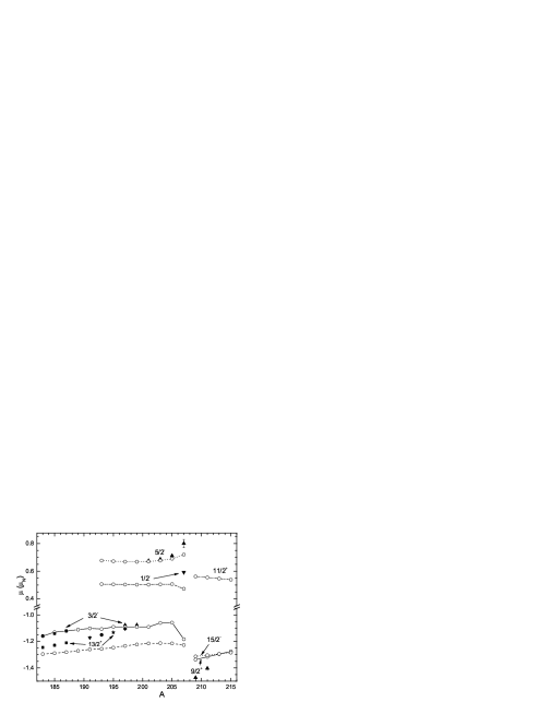
Figure 2: Magnetic moments of Pb isotopes. The experimental data are shown with filled triangles (up and down) Stone , squares Pb , filled circles Dutta , a star Dinger and a rhombus Anselment . Open circles show the theoretical predictions. The quantum numbers of the single-particle configurations assumed in the calculations are also indicated.

Table 2: Magnetic moments (in $\mu_{\rm N}$) of Pb isotopes. The experimental data are from Stone , Dutta $(^{a)})$, Dinger $(^{b)})$ and Anselment $(^{c)})$. Those in preparation are given by Ref. Pb . The symbol * indicates excited states.

nucleus	neutron s.p. state $\lambda_{0}^{n}$	$\mu_{\rm exp}$	$\mu_{\rm Sch}$	$\mu_{\rm th}$	$\delta\mu$
${}^{183}{\rm Pb}$	$p_{3/2}$	Pb	-1.913	-1.139	-
${}^{185}{\rm Pb}$	$p_{3/2}$	Pb	-1.913	-1.130	-
${}^{187}{\rm Pb}$	$p_{3/2}$	Pb	-1.913	-1.121	-
${}^{197}{\rm Pb}$	$p_{3/2}$	-1.075(2)	-1.913	-1.090	-0.015(2)
${}^{199}{\rm Pb}$	$p_{3/2}$	-1.0742(12)	-1.913	-1.090	-0.016(1)
${}^{183}{\rm Pb}^{*}$	$i_{13/2}$	Pb	-1.913	-1.295	-
${}^{185}{\rm Pb}^{*}$	$i_{13/2}$	Pb	-1.913	-1.289	-
${}^{187}{\rm Pb}^{*}$	$i_{13/2}$	Pb	-1.913	-1.281	-
${}^{191}{\rm Pb}$	$i_{13/2}$	-1.172(7)	-1.913	-1.260	-0.088(7)
${}^{193}{\rm Pb^{a)}}^{*}$	$i_{13/2}$	-1.150(7)	-1.913	-1.256	-0.106(7)
${}^{195}{\rm Pb^{b)}}^{*}$	$i_{13/2}$	-1.1318(13)	-1.913	-1.247	-0.115(1)
${}^{197}{\rm Pb^{c)}}^{*}$	$i_{13/2}$	-1.105(3)	-1.913	-1.233	-0.128(3)
${}^{201}{\rm Pb}$	$f_{5/2}$	0.6753(5)	1.366	0.670	-0.005
${}^{203}{\rm Pb}$	$f_{5/2}$	0.6864(5)	1.366	0.677	-0.009
${}^{205}{\rm Pb}$	$f_{5/2}$	0.7117(4)	1.366	0.690	-0.022
${}^{207}{\rm Pb}^{*}$	$f_{5/2}$	0.80(3)	1.366	0.720	-0.08(3)
${}^{207}{\rm Pb}$	$p_{1/2}$	0.592585(9)	0.638	0.473	-0.120
${}^{209}{\rm Pb}$	$g_{9/2}$	-1.4735(16)	-1.913	-1.337	0.137(2)
${}^{211}{\rm Pb}$	$g_{9/2}$	-1.4037(8)	-1.913	-1.316	0.088(1)

Thus, for the chains of semi-magic Sn and Pb isotopes containing nuclides that are sufficiently far from the $\beta$-stability valley (the maximum value of the relative distance is $\varepsilon\simeq 25\%$), the two main assumptions of the calculation procedure, i.e. the spherical symmetry and one-quasiparticle approximation, work sufficiently well. The agreement between the theory and experimental data confirms also the universal character of the spin dependent parameters of the extended FFS theory which were found primarily for $\beta$-stable nuclei. Similar conclusions were obtained also in systematic studies of the $\beta$-decay properties of very neutron-rich nuclei Bo .

For completeness, we present also the magnetic moments of isotones with $N=82$, $Z_{\rm min}=51$ and $Z_{\rm max}=65$. They are collected in Table III and Fig.3. In this case, only the nuclei ¹³⁹La and ¹⁴¹Pr are $\beta$-stable, i.e. the $\beta$-stability valley for odd $N=82$ isotones has limits $Z_{\rm min}=57$ and $Z_{\rm max}=59$. Using the notation similar to the one introduced above, one finds $\delta Z_{-}=\delta Z_{+}=6$, and $\varepsilon^{\prime}_{-}\simeq\varepsilon^{\prime}_{+}\simeq 10\%$. It can be seen from Fig.3 and Table III that in terms of absolute deviation $\delta\mu$ the accuracy of the theoretical predictions is somewhat worse than for the isotopic chains analyzed above. Nevertheless, the theoretical results differ at most 15% from the experimental values. For some of these isotones which are rather close to the lanthanide deformed region the main assumptions of these calculations are not necessarily valid.

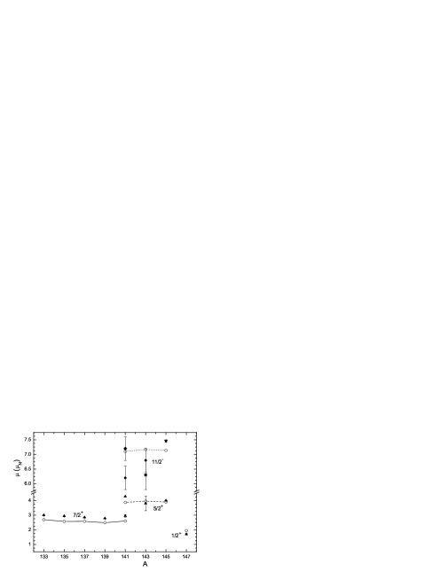
Figure 3: Magnetic moments of N=82 isotones.The experimental data are shown with filled triangles (up and down) Stone , filled circles Go12 , a rhombus Ej01 and a square Pr02 . Open circles show the theoretical predictions. The quantum numbers of the assumed single-particle configurations are also indicated.

Table 3: Magnetic moments (in $\mu_{\rm N}$) of N=82 isotones. The experimental data are from Stone , Go12 $(^{a)})$, Ej01 $(^{b)})$ and Pr02 $(^{c)})$. The symbol * indicates an excited state.

nucleus	proton s.p. state $\lambda_{0}^{p}$	$\mu_{\rm exp}$	$\mu_{\rm Sch}$	$\mu_{\rm th}$	$\delta\mu$
${}^{133}{\rm Sb}$	$g_{7/2}$	3.00(1)	1.817	2.693	-0.31(1)
${}^{135}{\rm I}$	$g_{7/2}$	2.940(2)	1.817	2.570	-0.370(2)
${}^{137}{\rm Cs}$	$g_{7/2}$	2.8513(7)	1.817	2.577	-0.274
${}^{139}{\rm La}$	$g_{7/2}$	2.7830455(9)	1.817	2.488	-0.295
${}^{141}{\rm Pr}^{*}$	$g_{7/2}$	2.95(9)	1.817	2.603	-0.35(9)
${}^{141}{\rm Pr}$	$d_{5/2}$	4.2754(5)	4.793	3.871	-0.404
${}^{143}{\rm Pm}$	$d_{5/2}$	3.8(5)	4.793	3.954	0.1(5)
${}^{145}{\rm Eu}$	$d_{5/2}$	3.999(3)	4.793	3.894	-0.105(3)
${}^{141}{\rm Pr^{a)}}^{*}$	$h_{11/2}$	6.2(4)	7.793	7.103	0.9(4)
${}^{141}{\rm Pr^{b)}}^{*}$	$h_{11/2}$	7.2(4)	7.793	7.103	-0.1(4)
${}^{143}{\rm Pm^{a)}}^{*}$	$h_{11/2}$	6.8(4)	7.793	7.168	0.4(4)
${}^{143}{\rm Pm^{c)}}^{*}$	$h_{11/2}$	6.3(5)	7.793	7.168	0.9(5)
${}^{145}{\rm Eu}^{*}$	$h_{11/2}$	7.46(4)	7.793	7.141	-0.32(4)
${}^{147}{\rm Tb}$	$s_{1/2}$	1.70(5)	2.793	1.942	0.24(5)

III The copper chain

Now we consider an example of a chain of non-magic isotopes, the copper one. It contains 11 odd isotopes, from ⁵⁷Cu to ⁷⁷Cu ($N_{\rm min}=28$, $N_{\rm max}=48$). In this case, two isotopes are $\beta$-stable, ^63,65Cu, i.e. we have $N^{\beta}_{\rm min}=$34, $N^{\beta}_{\rm max}=36$. The corresponding characteristics of the neutron excess and deficiency are equal to $\delta N_{+}=12$, $\varepsilon_{+}=33.3\%$, $\delta N_{-}=6$, $\varepsilon_{-}=17.6\%$. Thus, although the absolute value of the distance from the $\beta$-stability valley is less than that for the semi-magic chains considered in the previous section, the relative neutron excess is now maximal. Seven of these isotopes, ^57-69Cu, belong to the $2p-1f$ shell, while in the isotopes ^71-77Cu, the next higher $1g_{9/2}$ shell is filling. A systematic analysis of the properties of nuclei of the $2p-1f$ shell within the many-particle SM was carried out before Brown . Unfortunately, this paper contains only three isotopes of the Cu chain, i.e. with $A=61,63,65$.

We now analyzed the entire Cu isotopic chain using different assumptions.A comparison of the calculated values with experimental data Stone ; Isolde_Cu ; Cu_1 ; UliKos is given in Table 4 and displayed in Fig. 4.

III.1 Spherical calculations for copper chain

First, one can see that the spherical calculations performed within the same one-quasiparticle scheme as above (column 6 of Table 4 and open circles labelled $|3/2^{-}\rangle$(spher) in Fig.4) may have some relevance only in the middle of the chain, i.e. near A=69 corresponding to the magic number N=40. For ^61-65Cu, the full fp-space predictions within the many-particle SM Brown (column 5) are in perfect agreement with the data. The fact that the simple FFS theory calculations deviate from the experimental data indicates that many-particle admixtures should be taken into account in this region. The magicity of N=40 and related characteristics of the low-lying quadrupole excitations were discussed in Kaneko . Our spherical calculation gives some grounds to assume an onset of deformation in ^57,59,73Cu, this possibility will be discussed in the section D. For ⁷⁵Cu and ⁷⁷Cu isotopes, the experimental ground state $I^{\pi}$ values and magnetic moments can in principle be measured.

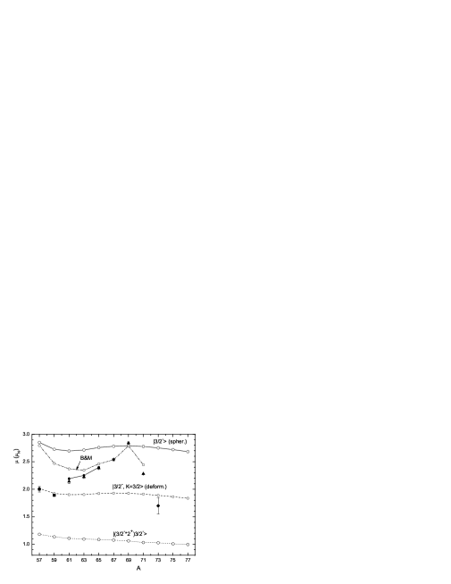
Figure 4: Magnetic moments of Cu isotopes. The experimental data are shown with filled triangles Stone , a filled pentagon Minam , a filled square Isolde_Cu , a filled star RiStone , or a filled rhombus UliKos . Theoretical values from Brown ($I=3/2$) are shown with filled circles. The assumed configurations are indicated for spherical, deformed and phonon-particle configurations, correspondingly (see details in text).

III.2 Particle-phonon coupling calculations

Among the relevant mechanisms of renormalization of the magnetic moments in spherical nuclei one should consider the correction induced by the virtual excitation of the low-laying states (the “phonons”). A consistent calculation of such contributions with the many-body theory methods is very complicated. Up to now, it was accomplished into practice only for magic nuclei where pairing is absent KhS . As an approximate version, we use the simple particle-phonon coupling model Bohr2 developed for the magnetic moment problem by I. Hammamoto Hammam . In this model, the unperturbed ground state $|jm>$ of the odd nucleus under consideration is mixed with the unperturbed particle-phonon one,

$$|(jL)jm>=\sum\limits_{M}C^{jm}_{jm-M\,LM}|jm-M>\,|LM>\,,$$ (1)

where $L$ is the phonon multipolarity. The magnetic moment of such “bare” state is equal to

$$\mu_{p+ph}=<(jL)jj|\,\hat{\mu}^{z}_{p}+\hat{\mu}^{z}_{ph}\,|(jL)jj>\,,$$ (2)

where $\hat{\mu}^{z}_{ph}$ stands for the 3-rd component of the phonon magnetic moment operator $\hat{\boldsymbol{\mu}}_{ph}=g_{R}\hat{\bf L}$, with $g_{R}$ being the phonon gyromagnetic ratio. In the collective model used in Hammam , one has $g_{R}=Z/A$. A simple calculation yields

$$\mu_{p+ph}=\left[1-\frac{L(L+1)}{2j(j+1)}\right]\mu_{p}+\frac{L(L+1)}{2(j+1)}g_{R}\,.$$ (3)

As we will see, for the Cu nuclei the admixture of the particle-phonon state is often large, and therefore the perturbation theory used in Hammam is not valid in this case. Instead, one could solve the two-level problem we deal with here exactly. The dynamical admixture of the two states under consideration is

$$\widetilde{|jm>}=c_{1}|jm>+c_{2}|(jL)jm>\,.$$ (4)

The corresponding magnetic moment is

$$\tilde{\mu}_{p}=(1-w)\mu_{p}+w\mu_{p+ph}\,,\quad w=|c_{2}|^{2}=1-|c_{1}|^{2},$$ (5)

or

$$\tilde{\mu}_{p}=\mu_{p}-w\left[\frac{L(L+1)}{2j(j+1)}\mu_{p}-\frac{L(L+1)}{2(j+1)}g_{R}\right]\,.$$ (6)

For the Cu isotopes under consideration the $2^{+}_{1}$-state contribution dominates, such that for $\lambda_{0}=p_{3/2}$ we have $j=3/2\,,L=2$, and

$$\tilde{\mu}_{p}=\mu_{p}-w\left(\frac{4}{5}\mu_{p}-\frac{6}{5}g_{R}\right)\,.$$ (7)

To indicate the maximal impact of the particle-phonon coupling we display in Fig. 4 the results for the maximum value of the phonon mixing amplitude $w=1$ (i.e. the open circles labelled as $|(3/2^{-}*2^{+})3/2^{-}\rangle$). Next, for each nucleus we calculated the value of $w$ which brings the magnetic moment into agreement with experiment. These values are given in the 7-th column of Table 4. It shows that near $A=69$ the required phonon mixing amplitude is reasonably small (i.e. $w$ = 15–30%). On the wings of the chain $w$ $\geq$ 50%. In such a situation, the model used is evidently irrelevant. At the left wing of the chain, as well as at the right wing in the case of the $I^{\pi}=3/2^{-}$ configuration, this can be interpreted as an indication for the appearance of a stable ground state deformation.

III.3 A simple estimate of the phonon admixture within the Bohr-Mottelson model

A realistic estimate of the phonon admixture can also be obtained within the collective Bohr-Mottelson (BM) model Bohr2 in terms of the excitation energy $\omega_{L}$ and transition probability $B(EL)$ of the collective state under consideration. Within this model, the particle-phonon interaction matrix element reads:

$$h(j_{1},(j_{2}L)j_{1})=(-1)^{L}\left(\frac{2L+1}{4\pi}\right)^{1/2}C^{j_{2}\frac{1}{2}}_{j_{1}\frac{1}{2}\,L0}\left(\frac{\omega_{L}}{2C_{L}}\right)^{1/2}<j_{2}|k_{L}(r)|j_{1}>\,,$$ (8)

where $C_{L}$ is the stiffness coefficient of the $L$-th vibration related to the vibration amplitude $\beta_{L}$ via

$$\beta_{L}=\sqrt{2L+1}\left(\frac{\omega_{L}}{2C_{L}}\right)^{1/2},$$ (9)

and $k_{L}(r)$ stands for the radial form factor which for surface vibrations has the form:

$$<j_{2}|k_{L}(r)|j_{1}>\approx\left<j_{2}\left|R_{0}\frac{\partial U}{\partial r}\right|j_{1}\right>\,.$$ (10)

For the states in the vicinity of the Fermi level of the Cu isotopes these matrix elements are approximately equal to 50 MeV. Inserting now in Eq. (8) $L$=2, $j_{1}$=$j_{2}$ =3/2, and using Eqs.  (9) and (10), one obtains a simple formula for the Cu isotopes:

$$<h>\approx\frac{\beta}{\sqrt{20\pi}}\,50\,[\mbox{MeV}]=6.31\beta[\mbox{MeV}]\,.$$ (11)

Using the exact solution for the two-level problem, one finds for the mixing probability

$$w_{\rm BM}=\frac{|<h>|^{2}}{\left(\frac{\omega}{2}+\sqrt{\frac{\omega^{2}}{4}+|<h>|^{2}}\right)^{2}+|<h>|^{2}}\,.$$ (12)

We calculated values of $w_{\rm BM}$ (column 8 in Table 4) for the ^57-71Cu isotopes for which the experimental values of $\omega_{2}$ and $\beta_{2}$ in the even-even Ni core are known (see Table V). The last positions of the columns 8 and 9 are empty as the corresponding data on the $2_{1}^{+}$-excitation in the ⁷²Ni nucleus are absent. To avoid double-counting of the effect, one should take into account that the $2^{+}$-phonon admixture is partially taken into account in the FFS theory equations via the local quasiparticle charge $e_{q}$. On the basis of the analysis of the magnetic moment of ⁶⁹Cu, the odd neighbor of the magic nucleus ⁶⁸Ni, we find that the value of $\mu_{p}$ in (6) should be multiplied with the factor 1.05 (see BST ). Taking this into account and using the values for $w_{BM}$, Eq. 6 then yields the magnetic moments values that are marked in Fig. 4 with the label B&M. As one can see, the BM model helps to explain deviations from the one-quasiparticle approximation result for nuclei in the vicinity of ⁶⁹Cu, the corresponding even-even core being close to ⁶⁸Ni. Indeed, in this case the phonon admixture coefficients $w_{\rm BM}$ predicted by the BM model (column 8 of Table 4) are quite close to the ones “required” to fit to data (the 7-th column of this table). This indicates the relevance of the particle-phonon coupling mechanism in this region of the Cu chain. On the other hand, for the ^57,59Cu isotopes the values of $w_{\rm BM}$ are much smaller than $w$, the latter being unrealistically large for these two isotopes. This indicates that the particle-phonon mechanism is irrelevant in the vicinity of the magic core ⁵⁶Ni.

Finally, it is of interest to mention that the calculations for the isotopes with $A=61-65$ are in qualitative agreement with those within the many-particle SM Brown , indicating that the 2${}^{+}_{1}$-state admixture dominates among the many-particle configurations.

Table 4: Magnetic moments (in $\mu_{\rm N}$) of Cu isotopes. The experimental data are from Stone , Minam $(^{a)})$, Isolde_Cu $(^{b)})$, RiStone $(^{c)})$.

Nucleus	proton $\lambda_{0}$	$\mu_{\rm exp}$	$\mu_{\rm Sch}$	$\mu_{\rm th}$Brown	$\mu_{\rm th}$	$w$	$w_{\rm BM}$	$\mu_{\rm th}$+$\delta\mu_{\rm BM}$
${}^{57}{\rm Cu^{a)}}$	$p_{3/2}$	2.00(5)	3.793	—	2.850	0.51	0.11	2.794
${}^{59}{\rm Cu^{b)}}$	$p_{3/2}$	1.891(9)	3.793	—	2.726	0.53	0.23	2.470
${}^{61}{\rm Cu}$	$p_{3/2}$	2.14(4)	3.793	2.193	2.695	0.35	0.27	2.370
${}^{63}{\rm Cu}$	$p_{3/2}$	2.2273	3.793	2.251	2.713	0.30	0.29	2.346
${}^{65}{\rm Cu}$	$p_{3/2}$	2.3816 (2)	3.793	2.398	2.759	0.23	0.24	2.460
${}^{67}{\rm Cu^{c)}}$	$p_{3/2}$	2.54(2)	3.793	—	2.781	0.14	0.21	2.536
${}^{69}{\rm Cu}$	$p_{3/2}$	2.84(2)	3.793	—	2.789	0	0.075	2.789
${}^{71}{\rm Cu}$	$p_{3/2}$	2.28(1)	3.793	—	2.778	0.30	0.26	2.444
${}^{73}{\rm Cu}$	$p_{3/2}$	UliKos	3.793	—	2.752	$\simeq$0.60	—	—

III.4 Calculations for copper chain assuming deformation

Let us now carry out an alternative calculation supposing these Cu isotopes to be deformed. To estimate the possible impact of the quadrupole deformation on the magnetic moments one may assume a simple rigid rotor picture Bohr with the effective rotational g-factor being the one for a uniformly charged rigid body $g_{R}=Z/A$ and the intrinsic g-factor $g_{K}=\mu_{j}/j$, where $\mu_{j}$ stands for the magnetic moment of the odd quasiparticle in the spherical core. In fact, such an approximation accounts only for a change of the kinematic factors in the case of a deformed core due to the precession of the rotational and intrinsic angular momenta with respect to the total angular momentum. As seen from Fig. 4 (open circles labelled with $|3/1^{-},K=3/2\rangle$ (deform), this simplest model leads to a qualitative agreement with the data for the nuclei at the left wing of the chain, i.e. for the neutron-deficient ^57,59Cu isotopes. As to the right wing with the neutron-rich ^73-77Cu isotopes, the situation is less clear. Only for ⁷³Cu ($I^{\pi}=3/2^{-}$) an experimental moment value is available and the “deformed” calculation practically agrees with the experiment. Note that the systematic calculations HF predict a significant $\beta_{2}$ deformation for the ^73-77Cu isotopes. At the same time, according to this systematic, the nuclei in the middle of the shell ($63<A<73$) are relatively weakly deformed. Therefore, this rough model is obviously not justified for those nuclei. On the other hand, the fact that the many-particle SM calculations for the three Cu isotopes in the vicinity of N=40 (i.e. A = 61-65; filled circles in Fig. 4) Brown are in agreement with the experimental data may give evidence that these nuclei are nearly spherical but that the weight of many-particle configurations in the ground-state is rather high. It were very instructive to carry out similar many-particle SM calculations for the other Cu isotopes belonging to the $2p-1f$ shell.

Table 5: Main 2${}_{1}^{+}$-state characteristics in even Ni isotopes BE2 ; Sor ; Per

A	$\omega_{2_{1}^{+}}$ (keV)	B(E2)$\uparrow$ (W.U.)	$\beta$
56	2700.6(7)	9.4(19)	0.173(17)
58	1454.0(1)	10.4(3)	0.1828(26)
60	1332.518(5)	13.4(2)	0.2070(17)
62	1172.91(9)	12.2(3)	0.1978(28)
64	1345.75(5)	10.0(11)	0.179(9)
66	1425.1(3)	7.8(11)	0.158(12)
68	2033.2(2)	3.2(7)	0.100(12)
70	1259.6(2)	9.9(1.6)	0.178(15)

III.5 The nuclei at the extremes of the Cu chain

A different situation takes place in the vicinity of the even-even core ⁵⁶Ni which could in principle be considered as “doubly magic”, but in fact $N=28$ and $Z=28$ turn out to be a bad sequence of magic numbers. Spectroscopic studies Rud ; Johan have revealed evidence for two well-deformed excited bands in ⁵⁶Ni. The first rotational band can be explained within shell-model calculations in the full pf model space while the second one seems to be related to the excitations into the $1g_{9/2}$-orbit Horoi . Actually, the isotope ⁵⁶Ni is so “soft” that it becomes deformed by addition of only one proton. As a result, the rotor-particle model explains the experimental value of its magnetic moment. In isotopes with large neutron excess, i.e. $A\geq$73, the deformation pattern is not so definite. Absence of the experimental data for $\omega_{2}$ and $B(E2)$ in the corresponding Ni isotopes does not permit to find the magnetic moment within the Bohr-Mottelson model. An attempt to use the phonon-particle model in this mass region shows that the adjusted value of the phonon admixture coefficient turns out to be unrealistically large (see Table 4). On the other hand, the particle-rotor model also explains the data only qualitatively. For more definite conclusions, it were instructive to examine the properties of the 2⁺-excitation in the core, ⁷⁶Ni, which is very close to the 3-rd semi-magic isotope ⁷⁸Ni. In addition, it were important to determine the $I^{\pi}$ values as well as the experimental magnetic moments for the ^75,77Cu nuclei.

Thus, with the above reservations, we see that examination of the magnetic moments of the long Cu isotope chain permits to retrace the evolution of the shape of the ground state, from spherical in the middle of the chain to deformed at the wings where the nuclei have a large neutron excess or neutron deficiency.

IV Conclusions and discussion

We have performed a systematic analysis of the magnetic moments of several long isotope and isotone chains of medium heavy and heavy nuclei. The modern version of the self-consistent FFS theory with exact account for the continuum has been used. The quasi-particle self-consistent basis is generated within the Generalized EDF method Fay . The extended Landau-Migdal effective interaction includes the spin-isospin tensor terms induced by the one-pion and one-rho-meson exchange. For the vast majority of the nuclei considered in the present work and in BST good agreement at the level of 0.1-0.2$\mu_{N}$ has been obtained. The best accuracy was achieved for the chains of the semi-magic lead and tin isotopes.

We analyzed also in detail the isotopic copper chain for which new data on magnetic moments were obtained recently Isolde_Cu ; Cu_1 . It includes nuclei far from the $\beta$–stability valley, with a maximal relative neutron excess, $\varepsilon_{+}=33\%$. Our study has shown that the analysis of magnetic moments of long isotopic chains of non-magic nuclei provides important information on the evolution of the ground state structure with neutron number. Copper nuclei can be described in terms of a proton added to the even-even Ni core. If, with some reservations, one considers $N=28$ and $Z=28$ as magic numbers, the Ni core chain will include two magic nuclei, ⁵⁶Ni and ⁶⁸Ni, ending with the isotope ⁷⁶Ni which is very close to the next magic nucleus ⁷⁸Ni. In the middle of the chain, in the vicinity of the ⁶⁸Ni core, magnetic moments are sufficiently well reproduced supposing the spherical symmetry of the ground state if the $2^{+}_{1}$-state virtual admixture is taken into account. In the wings of the chain predictions of the theory with the spherical basis differ significantly from the data. Qualitative agreement could be achieved when supposing the ground state to be deformed, in accordance with systematic calculations HF . Thus, a sharp change of the magnetic moment value under addition of a few nucleons may give a signal of a sudden change in nuclear structure. It should be noted that the situation for the ^75,77Cu isotopes is not clear as far as the ground state $I^{\pi}$ values are not definitely known experimentally in this case.

It is worth to stress that our conclusions about the structure of nuclei of the Cu chain has to be considered as preliminary in view of the fact that rather schematic models were used for the surface vibration admixture in the spherical case and also for deformed nuclei. It would be instructive to carry out calculations for the seven members of the chain which belong to the $2p-1f$ shell within the approach of Brown . It would be also of interest to perform the calculation of the magnetic moments within the hybrid approach uniting the many-particle SM and the FFS theory. So far, this method SKh has been applied only for the isolated 1$f_{7/2}$ shell.

It is interesting also to mention the possibility of a new type of phase transitions in nuclei which has recently been predicted by V.A. Khodel et al. KhC . It consists in a rearrangement of the Fermi system vacuum due to the merging of a pair of single-particle levels close to the Fermi surface. This phase transition results in partial occupation numbers and is analogous to the so-called fermionic condensation in infinite Fermi systems KhSh . According to estimations in KhC , such phase transition could occur in the $2p-1f$ nuclei. It would be of great interest to carry out an analysis of the magnetic moments supposing that such phase transition takes place.

The authors thank V.A. Khodel, A.N. Andreev and O.I. Ivanov and Y.A. Litvinov for valuable discussions and U. Koster for sending us his unpublished data.

This research was partially supported by the joint Grant of the Russian Fund for Basic Research (RFBR) and Fund for Scientific Research Flanders RFBR-Fl-05-02-19813, by the Grant NSh-3004.2008.2 of the Russian Ministry for Science and Education, by the RFBR grants 06-02-17171-a, 07-02-00553-a and by DFG, Germany via the contract No. 436 RUS 113907/0-1.

References

- (1) A. Bohr and B. R. Mottelson, Nuclear Structure (Benjamin, New York, 1971.), Vol. 1
- (2) A. B. Migdal, Theory of finite Fermi systems and applications to atomic nuclei (Wiley, New York, 1967).
- (3) N. J. Stone, ADNDT, 90, 75 (2005).
- (4) I. N. Borzov, E. E. Saperstein, S. V. Tolokonnikov, Phys. At. Nucl., to be published.
- (5) A. V. Smirnov, S. V. Tolokonnikov, S. A. Fayans, Sov. J. Nucl. Phys. 48, 1030 (1988).
- (6) S. A. Fayans, S. V. Tolokonnikov, E. L. Trykov, and D. Zawischa, Nucl. Phys. A676, 49 (2000).
- (7) S. Shlomo, G.F. Bertsch, Nucl. Phys., A243, 507 (1975).
- (8) E. E. Saperstein, S. V. Tolokonnikov, S. A. Fayans, Preprint KIAE-2571 (1975).
- (9) A. P. Platonov, E. E. Saperstein, Nucl. Phys. A486, 63 (1988).
- (10) N. I. Pyatov and S. A. Fayans. Sov. J. Part. Nucl. 14, 401 (1983).
- (11) I. N. Borzov, S. V. Tolokonnikov, and S. A. Fayans. Sov. J. Nucl. Phys. 40, 732 (1984).
- (12) K. Minamisono et al., Phys.Rev.Lett. 96, 102501 (2006)
- (13) V. V. Golovko, I. Kraev, T. Phalet, N. Severijns et al., Phys. Rev. C70, 014312 (2004).
- (14) K. T. Flanagan, G. Neyens et al. (in preparation).
- (15) U. Koster et al. (p.c., unpublished ISOLDE-RILIS data).
- (16) M. D. Seliverstov et al. (in preparation).
- (17) W. Kohn, L. J. Sham, Phys. Rev. A140, 1133 (1965).
- (18) Y. Aboussir, N. Pearson, A. K. Dutta, and F. Tondeur, ANDT 61, 127 (1995).
- (19) S. B. Dutta, R. Kirchner, O. Klepper et al., Z. Phys. A 341, 39 (1991).
- (20) U. Dinger, J. Eberz, G. Huber et al., Z. Phys. A 328, 253 (1987).
- (21) M. Anselment, W. Faubel, S. Goring et al. Nucl. Phys. A451, 471 (1986).
- (22) I. N. Borzov, Nucl. Phys. A777, 435 (2006).
- (23) B. I. Gorbachev, A. I. Levon, O. F. Nemts et al., Zh. Eksp. Teor. Fiz. 87, 3 (1984).
- (24) H. Ejiri, T. Shibata, M. Takeda, Nucl. Phys. A221 211 (1974).
- (25) H. Prade, L. Kaubler, U. Hageman et al., Nucl. Phys. A333, 33 (1980).
- (26) M. Honma, T. Otsuka, B. A. Brown, T. Mizusaki, Phys. Rev. C69, 034335 (2004)
- (27) K. Kaneko, M. Hasegawa, T. Mizusaki, Y. Sun, Phys. Rev. C74, 024321 (2006)
- (28) V. A. Khodel and E. E. Saperstein, Phys. Rep. 92, 183 (1982).
- (29) A. Bohr and B.R. Mottelson, Nuclear Structure (Benjamin, New York, Amsterdam, 1974.), Vol. 2.
- (30) I. Hammamoto, Phys. Lett. B61, 343 (1973).
- (31) J. Rikovska and N.J. Stone, Hyp. Int. 129, 131 (2000).
- (32) D. Rudolph, C. Baktash, M.J. Brinkman, E. Caurier et al., Phys. Rev. Lett. 82, 3763 (1999).
- (33) E.K. Johansson et al., Eur.Phys.J. A 27, 157 (2006).
- (34) M. Horoi, B. Brown, T. Otsuka et al., Phys. Rev. C73, 061305 (2006).
- (35) NNDC Databases, http://www.nndc.bnl.gov/be2
- (36) O. Sorlin, S. Leenhardt, C. Donzaud et al., Phys. Rev. Lett. 88, 092501 (2002).
- (37) O. Perry, O. Sorlin, S. Franchoo et al., Phys. Rev. Lett. 96, 232501 (2006).
- (38) E.E. Saperstein, V.A. Khodel, Yad. Fiz., 4, 701 (1966).
- (39) V. A. Khodel, J. W. Clark, Haotchen Li, and M. V. Zverev, Phys. Rev. Lett. 98, 216404 (2007).
- (40) V. A. Khodel, V. R. Shaginyan, JETP Lett.,51, 553 (1990).