Abstract

We study reversible quantum cellular automata with the restriction that these are also Clifford operations. This means that tensor products of Pauli operators (or discrete Weyl operators) are mapped to tensor products of Pauli operators. Therefore Clifford quantum cellular automata are induced by symplectic cellular automata in phase space. We characterize these symplectic cellular automata and find that all possible local rules must be, up to some global shift, reflection invariant with respect to the origin. In the one dimensional case we also find that every uniquely determined and translationally invariant stabilizer state can be prepared from a product state by a single Clifford cellular automaton timestep, thereby characterizing these class of stabilizer states, and we show that all 1D Clifford quantum cellular automata are generated by a few elementary operations. We also show that the correspondence between translationally invariant stabilizer states and translationally invariant Clifford operations holds for periodic boundary conditions.

1 Introduction

Classical cellular automata have become a standard modeling tool for complex phenomena. With their discrete time step and their intrinsically high degree of parallelization they are ideally suited for models of diverse phenomena as coffee percolation, highway traffic and oil extraction from porous media. As an abstract computational model cellular automata can simulate Turing machines, and even explicit simple automata such as Conway’s life game have been shown to support universal computation [1]. On the quantum side, the interest in cellular automata stems from their implementation in optical lattices and arrays of optical microtraps. However, the theory of quantum cellular automata (QCAs) is still in its early stage. Since each cell may influence several others, the dynamics is subject to a “no-cloning” constraint, leading to a non-trivial interplay between the conditions of locality and unitarity.

It is therefore helpful to have some class of QCAs, which can be analyzed in great detail, and which can serve as a testing ground for general ideas about QCAs. This paper is concerned with such an analysis, namely of the special class of Clifford quantum cellular automata (CQCAs), in which the elementary time step is given by a “Clifford gate”, meaning that it takes tensor products of Pauli matrices to tensor products of other Pauli matrices. In the theory of gate model computation, and for the one-way quantum computation model, a detailed analysis of what can be done with Clifford operations alone turned out to be very useful, even though – as the downside of allowing an efficient classical description – such gates alone do not allow universal quantum computation. By analogy it is therefore clear that CQCAs do not comprise the full complexity of QCAs. What one can hope to get, however, is an interesting class of cellular automata, and some tools for understanding this class in great detail.

A similar analysis has been done with Gaussian quantum cellular automata [3], e.g. the QCA describes a chain of harmonic oscillators with nearest neighbor couplings. For all these QCAs the Hilbert space of one elementary cell is infinite dimensional, and the QCA maps phase space translations, also referred to as Weyl operators, to phase space translations. In our approach we use elementary cells with a finite number of levels, which corresponds to replacing the continuous phase space by a discrete space.

1.1.  Definition of Clifford quantum cellular automata

By definition, a cellular automaton is a lattice system, which consists of many subsystems (called “cells”) labeled by a point lattice in space. For simplicity, we will always take the lattice as ${\mathbb{Z}}^{s}$, the integer cubic lattice in $s$ space dimensions. The cell systems in the classical case may have states like “occupied” and “empty”. In the quantum case, they will be $p$-state quantum systems, for some finite $p$. In either case the group of lattice translations (“shifts”) is a symmetry of the system.

The dynamics will be given by a discrete global time step, or global “transition rule” assumed to have the following three properties:

• translation invariance: the time step commutes with the lattice translation symmetries.

• reversibility: there is an inverse rule. For a finite quantum system this would mean unitary dynamics. For the infinite lattice system this will be stated algebraically below.

• locality, or “finite propagation speed”: the state of each cell after one step can be computed from the state in a fixed finite region around the cell.

These assumption define the class of reversible QCAs [2]. The locality and reversibility conditions are best phrased in the Heisenberg picture: if $A$ denotes some observable of the system, its expectation after one time step starting from the initial state $\rho$ will be $\langle T(A)\rangle_{\rho}$ for a suitable observable $T(A)$, where by $\langle A\rangle_{\rho}$ we denote the expectation of $A$ in the state $\rho$. The transformation $A\mapsto T(A)$ is what we will call the global rule of the automaton. Then reversibility (together with complete positivity, which is required of any dynamical map) implies that $T$ is a homomorphism of the observable algebra of the whole system: $T$ is linear, $T(AB)=T(A)T(B)$, and $T(A^{\ast})=T(A)^{\ast}$. Locality means that an observable $A_{x}$ localized at some lattice point $x\in{\mathbb{Z}}^{s}$ (i.e., an observable of the cell at $x$) will be mapped to an observable localized in the region $x+{\cal N}$. That is, $T(A_{x})$ will be in the tensor product of the cell algebras belonging to the sites $x+n$ with $n\in{\cal N}$. By translation invariance this set ${\cal N}$, called the neighborhood scheme of the automaton is independent of $x$.

The global transition rule $T$ is a map on an infinite dimensional space, and hence not readily specified explicitly. However, by using the basic properties of QCAs one can see that it suffices to know just a few local data, associated with the region ${\cal N}$, in order to reconstruct $T$ uniquely. Suppose we know $T(A_{x})$ for every observable $A_{x}$ in some basic cell $x$. Then by translation invariance we know the analogous transformation for any cell. Moreover, since every local observable can expanded in products of one-cell observables, and because $T$ is a homomorphism, we can compute $T$ for any local observable. So the restriction $T_{x}$ of $T$ to the observables of a single cell $x$ can be called the local rule of the automaton. We can also decide by a finite set of equations, whether a proposed local rule actually belongs to a well-defined global rule: clearly $T_{x}$ must be a homomorphism. The only further condition one has to check is that the images of observables $A_{x}$ and $B_{y}$ localized in the cells indicated also commute, i.e., $T_{x}(A_{x})T_{y}(B_{y})=T_{y}(B_{y})T_{x}(A_{x})$, whenever $x\neq y$. This is necessary, because $A_{x}$ and $B_{y}$ commute, and a moment’s reflection shows that this is also sufficient for uniquely reconstructing the images of arbitrary observables under $T$. The commutation conditions on the local rule are trivially satisfied when $x$ and $y$ are sufficiently far apart, when $x+{\cal N}$ and $y+{\cal N}$ are disjoint. Hence only finitely many conditions need to be checked.

For special classes, the job of specifying a QCA via its local rule can be reduced still further, which is where the Clifford condition comes in. Let us assume now that we have a qubit system, so the local cell dimension is $p=2$. For each local cell we thus have a basis for the observables, consisting of the identity and the three Pauli matrices, which we denote by $X,Y$ and $Z$. By $X_{x}$ etc. we denote the corresponding Pauli matrix belonging to the cell $x$. Finite tensor products of Pauli matrices belonging to different sites, perhaps with a sign $\pm 1,\pm i$ will be referred to as Pauli products. These form a group, called the Pauli group. Then a Clifford quantum cellular automaton (CQCA for short) is defined by the condition

• Clifford condition: If $A$ is any multiple of a Pauli product, so is $T(A)$.

Clearly, this is equivalent to the property that one-cell Pauli operators are taken to Pauli products, which simplifies the local rule. Moreover, it suffices to specify $T(X_{x})$ and $T(Z_{x})$ for some $x$, because we can compute $T(Y_{x})=T(iX_{x}Z_{x})=iT(X_{x})T(Z_{x})$ via the homomorphism property. Hence a CQCA is defined in terms of just two Pauli products.

Example 1.1.

For the one-dimensional lattice ($s=1$), consider the relations

$$\begin{array}[]{lclcr}T(X_{x})&=&&-Z_{x}&\\ T(Z_{x})&=&Z_{x-1}\otimes&X_{x}&\otimes Z_{x+1}\end{array}$$ (1)

Let us verify that all requirements for a local rule are satisfied. To begin with each of the expressions on the right hand side, as a product of Pauli matrices, is hermitian with square one. These are all the required conditions related to just a single line, and are satisfied for any Pauli product with a sign $\pm 1$. Next we have to verify the anti-commutation relation arising from applying a homomorphism $T$ to the anti-commutation relation $XZ+ZX=0$. Indeed, $T(X_{x})T(Z_{x})+T(Z_{x})T(X_{x})=-Z_{x-1}\otimes(Z_{x}X_{x}+X_{x}Z_{x})\otimes Z_{x+1}=0$. Hence the definition $T(Y_{x})=iT(X_{x})T(Z_{x})$ again produces a hermitian operator with square $\openone$, and the local rule is a homomorphism $T_{x}$ into the algebra on the sites $x+{\cal N}$ with ${\cal N}=\{-1,0,1\}$. Finally, we have to check the commutation rules for the images of observables from neighboring sites. For example, we have $[T(X_{x}),T(Z_{x+1})]=-[Z_{x},Z_{x}\otimes X_{x+1}\otimes Z_{x+2}]=0$, and similarly $[T(Z_{x}),T(Z_{x+2})]=0$. Perhaps the only non-trivial relation to check is

$$[T(Z_{x}),T(Z_{x+1})]=[Z_{x-1}\otimes X_{x}\otimes Z_{x+1},Z_{x}\otimes X_{x+1}\otimes Z_{x+2}]=0,$$

which holds because the factors on sites $x$ and $x+1$ both anti-commute.

In principle, we would also have to check the existence of an inverse for the automaton, which is actually given by $T(X_{x})=X_{x-1}\otimes Z_{x}\otimes X_{x+1}$ and $T(Z_{x})=-X_{x}$, but as was shown in [2], this already follows from the homomorphism property. $\lozenge$

It is clear from this example that the search for CQCAs is now a combinatorial problem. We can first look for self commuting Pauli products, i.e., Pauli products, which commute with all translates of itself. Only these can appear on the right hand side of local rules. One can then check, for any pair $X^{\prime},Z^{\prime}$ of such products, whether they anti-commute, while all proper translates of $X^{\prime}$ commute with $Z^{\prime}$. In fact, we began our investigation by running this simple search program. We found, for example, that while there is a rich variety of self-commuting Pauli products only reflection symmetric products could appear in a local rule. This will indeed be shown in full generality below.

1.2.  Translationally invariant stabilizer states

Commuting sets of Pauli products also play a central role in the problem of determining so-called stabilizer states: these are pure states, which can be characterized by eigenvalue equations for Pauli products or, equivalently, by the condition that certain Pauli products have expectation $\pm 1$. It is easy to check that Pauli products which simultaneously have sharp expectations $\pm 1$ must commute. Now for the infinite lattice systems it is natural to ask which Pauli products $A$ have the property that there is a unique pure state $\rho$ of the infinite system, which has expectation 1 for $A$ and all its translates.

As the simplest example, let us take $A=Z_{x}$, so we ask for states with $\langle Z_{x}\rangle=1$ for all $x\in{\mathbb{Z}}^{s}$. Clearly, this defines the “all spins up” state, which is an infinite product state. A slightly more complex example uses the stabilizer operators $A=Z_{x-1}\otimes X_{x}\otimes Z_{x+1}$, which singles out the one-dimensional cluster state, whose higher dimensional analogs are used as the entanglement resource for universal one-way quantum computing [5].

Showing that these eigenvalue equations define a unique state of the infinite lattice is now very easy, by using the cellular automaton (1): Since this automaton maps $Z_{x}$ to the required stabilizer operator, all existence and uniqueness problems for such a state are mapped to the corresponding trivial questions for the stabilizer operator $Z_{x}$. In other words, self-commuting Pauli products of the form $A=T(Z_{x})$ for some CQCA $T$ characterize a unique translation invariant cluster state. We will show later that (at least in one dimension) the converse is also true, so that there is a very close connection between stabilizer states and Clifford cellular automata.

1.3.  Our methods and techniques

The definition of CQCAs given above applies only to qubit systems. However, all our results are also valid for higher dimensional cells, particular cells of prime dimension $p$. The role of the Pauli operators $X$ and $Z$ is then taken by the cyclic shift on ${\mathbb{C}}^{p}$, and the multiplication by a phase, i.e.

$$\begin{array}[]{lcr}X|q\rangle&=&|q+1\rangle\\ Z|q\rangle&=&{\rm e}^{2\pi iq/p}|q\rangle,\end{array}$$ (2)

where all ket labels $q$ are taken modulo $p$. Products of these operators are called Weyl operators, and the appropriate definition of CQCAs requires that $T(X_{x})$ and $T(Z_{x})$ are both tensor products of Weyl operators. The necessary preliminaries on the Pauli group and Clifford operations in this extended setting, and the background concerning infinite lattice systems are provided in Subsection 2.1.

In order to utilize the translation symmetry one would like to use Fourier transform techniques. However, in the discrete structures an integral with complex phases makes no sense. It turns out, however, that a “generating function” technique does nearly as well. The analogue of the Fourier transform is then a Laurent-polynomial in an indeterminate variable, i.e., a polynomial with coefficients in the field ${\mathbb{Z}}_{p}={\mathbb{Z}}_{p}$ with both positive and negative powers. The salient facts about this structure will be provided in Subsection 2.3.

The description in terms of Laurent polynomials can also be adapted to lattices with periodic boundary conditions. This will be described in Section 4.

1.4.  Outline and summary of results

In order to discuss general Clifford quantum cellular automata, that is, for arbitrary lattice and single cell dimension, we introduce in Section 2 the necessary mathematical tools. We first review the concept of discrete Weyl systems and (infinite) tensor products of them, thereby characterizing the underlying “phase space”. We show that Clifford QCAs can be completely characterized in terms of classical symplectic cellular automata. We also introduce our Fourier transform techniques and study the structure of isotropic subspaces, because these play an essential role for the characterization of symplectic cellular automata and translationally invariant stabilizer states.

In Section 3 we will state our main results. We show that symplectic cellular automata can be identified with two-by-two matrices, which have Laurent-polynomials as matrix elements. We will find that the determinant of this matrix must be one and that the polynomials must be reflection invariant. In the one-dimensional case we state that every translationally invariant stabilizer state can be prepared out of a product state by a single CQCA step. Furthermore, we also specify the generators of all 1D QCAs.

Finally, we show in Section 4 that the close connection between translationally invariant stabilizer states and CQCAs also holds in the case of periodic boundary conditions even in every lattice dimension.

2 Mathematical tools

We introduce some mathematical tools, which we will use to study Clifford QCAs. We start with a short repetition of finite Weyl systems, which generalize the Pauli operators to systems with prime number dimensions. These Weyl operators can be described by phase space vectors and Clifford operations are induced by symplectic transformations on the phase space. Since we are looking for translationally invariant operations, we also introduce some kind of Fourier transform.

2.1.  Weyl algebras

Each single cell in a QCA is given by a finite dimensional quantum system, so the observables on a single system can be described by matrices from the algebra ${\cal M}_{p}({\mathbb{C}})$. A possible basis for this algebra is given by Weyl operators ${\bf w}(r,k)=X^{r}Z^{k}$, whereby $X$ and $Z$ are given by the generalized Pauli operators from equation (2). These operators fulfill the Weyl relations

$${\bf w}(r_{1}+r_{2},k_{1}+k_{2})=\varepsilon^{-r_{2}k_{1}}{\bf w}(r_{1},k_{1}){\bf w}(r_{2},k_{2})\,,$$ (3)

where $\varepsilon=\exp(2\pi{\rm i}/p)$ is the $p^{\rm th}$ root of unity. ¿From this equation the commutation relation

$${\bf w}(r_{1},k_{1}){\bf w}(r_{2},k_{2})=\varepsilon^{r_{1}k_{2}-r_{2}k_{1}}{\bf w}(r_{2},k_{2}){\bf w}(r_{1},k_{1})$$ (4)

immediately follows. Obviously we get for $p=2$ the standard Pauli operators from

$$X={\bf w}(1,0)\,,\quad Y=i{\bf w}(1,1)\,,\quad Z={\bf w}(0,1)\;,$$ (5)

and the Weyl operators are generalizations of the Pauli operators to higher dimensional spaces. The indices $r$ and $k$ are integers modulo $p$, so they are elements of the finite field ${\mathbb{F}}={\mathbb{Z}}_{p}$. In infinite dimensional systems Weyl operators describe phase space translations and therefore we call the space ${\mathbb{F}}^{2}$ a discrete phase space.

Building a tensor product of Weyl operators means that we must assign a phase space vector $\xi(x)=(\xi_{+}(x),\xi_{-}(x))\in{\mathbb{F}}^{2}$ to each lattice point $x\in{\mathbb{Z}}^{s}$, so $\xi$ is a mapping from ${\mathbb{Z}}^{s}$ into ${\mathbb{F}}^{2}$ and we denote for the tensor product

$${\bf w}(\xi)=\bigotimes_{x\in{\mathbb{Z}}^{s}}{\bf w}(\xi(x))\;.$$ (6)

This infinite tensor product is well defined, if there are only finitely many of the Weyl operators different from $\openone={\bf w}(0)$. For a mapping $\xi:{\mathbb{Z}}^{s}\to{\mathbb{F}}^{2}$ we have that only finitely many $x$ with $\xi(x)\neq 0$ are allowed, so the support of $\xi$ is finite. The set of such functions describes the global system and is identified with the global phasespace $\Xi_{s}$. We denote the finitely supported functions from ${\mathbb{Z}}^{s}$ to ${\mathbb{F}}$ by $C_{{\mathbb{F}}}({\mathbb{Z}}^{s})$ and we have $\Xi_{s}=C_{{\mathbb{F}}}({\mathbb{Z}}^{s})^{2}$. The corresponding Weyl operators generate an algebra and, by restricting the support of the functions to some finite subset $\Lambda\in{\mathbb{Z}}^{s}$, we get a finite dimensional algebra $\mathcal{A}(\Lambda)=\bigotimes_{x\in\Lambda}{\cal M}_{p}({\mathbb{C}})$, also called the local algebra of $\Lambda$. By taking the union of these algebras over all finite subsets of ${\mathbb{Z}}^{s}$ and taking the closure (in operator norm) we get a quasilocal $C^{\ast}$-algebra $\mathcal{A}$ [6], which is used in the general theory of quantum cellular automata [2].

The local structure is accompanied by the symmetry group of lattice translations. For each lattice translation $x\in{\mathbb{Z}}^{s}$ an automorphism $\alpha_{x}$ is defined by

$$\alpha_{x}{\bf w}(\xi)={\bf w}(\tau_{x}\xi)\;.$$ (7)

where $\tau_{x}$ is the translation of phase space vectors. Given a phase space vector $\xi$, the translated vector is $(\tau_{x}\xi)(y)=\xi(y-x)$. So the automorphism $\alpha_{x}$ shifts the position of each tensor factor by $x$. It follows directly from (7) that the homomorphism property $\alpha_{x+y}=\alpha_{x}\alpha_{y}$ holds. Furthermore, the automorphism $\alpha_{x}$ maps the local algebra $\mathcal{A}(\Lambda)$ onto $\mathcal{A}(\Lambda+x)$.

The Weyl relations of a single system completely determine the relations of the global system which are given by

$${\bf w}(\xi+\eta)=\varepsilon^{\beta(\xi,\eta)}{\bf w}(\xi){\bf w}(\eta)\;,$$ (8)

where we have introduced the bilinear form $\beta(\xi,\eta):=\sum_{x\in{\mathbb{Z}}^{s}}\xi_{+}(x)\eta_{-}(x)$. The adjoint of a Weyl operator is given by

$${\bf w}(\xi)^{\ast}=\varepsilon^{-\beta(\xi,\xi)}{\bf w}(-\xi)$$ (9)

which is due to the unitarity of the Weyl operators.

Since commutation relations are essential for validating possible local rules of quantum cellular automata, the commutation relations of Weyl operators are most important for us. We get

$${\bf w}(\eta){\bf w}(\xi)=\varepsilon^{\sigma(\xi,\eta)}{\bf w}(\xi){\bf w}(\eta)\;,$$ (10)

whereby $\sigma(\xi,\eta):=\beta(\xi,\eta)-\beta(\eta,\xi)$ is the canonical symplectic form on $\Xi_{s}$. This means that two Weyl operators ${\bf w}(\xi)$ and ${\bf w}(\eta)$ are commuting if and only if $\sigma(\xi,\eta)=0$ (and for $p=2$ they anti-commute if $\sigma(\xi,\eta)=1$). In particular, an abelian algebra of Weyl operators is given by a subspace of $\Xi_{s}$ on which the symplectic form vanishes. Such a subspace is called isotropic and a maximally abelian algebra corresponds to a maximally isotropic subspace.

2.2.  Clifford quantum cellular automata

As already mentioned a Clifford quantum cellular automaton is a QCA which maps Weyl operators to multiples of Weyl operators, which are in our case tensor products of single cell Weyl operators, so we have the relation (the “Clifford condition”)

$$T({\bf w}(\xi))=\vartheta(\xi){\bf w}({\bf t}\xi)\;$$ (11)

with a mapping ${\bf t}$ on the phase space $\Xi_{s}$ and some phase valued function $\vartheta:\Xi_{s}\to\mathcal{U}(1)=\{z\in{\mathbb{C}}||z|=1\}$. Since $T$ is an automorphism we find with equation (10) that ${\bf w}({\bf t}\xi){\bf w}({\bf t}\eta)=\varepsilon^{\sigma(\eta,\xi)}{\bf w}({\bf t}\eta){\bf w}({\bf t}\xi)$ holds, so we have $\sigma({\bf t}\xi,{\bf t}\eta)=\sigma(\xi,\eta)$ or in other words ${\bf t}$ is a symplectic transformation.

For reversible operations the Clifford condition is in general equivalent to the Weyl covariance (for general theory on covariant channels we refer to [7] and for the special case of Weyl covariance to [8, 9]) of the quantum channel:

Proposition 2.1.

An automorphism $T$ on the Weyl algebra $\mathcal{A}$ fulfills the Clifford condition (11) if and only if the Weyl covariance

$$T({\bf w}(\eta)A{\bf w}(\eta))={\bf w}({\bf t}\eta)T(A){\bf w}({\bf t}\eta)^{\ast}\quad\forall\eta\in\Xi_{s}$$ (12)

holds for all operators $A\in\mathcal{A}$ and some symplectic transformation ${\bf t}$.

Proof.

Because the Weyl operators form a basis of $\mathcal{A}$ we just have to insert ${\bf w}(\xi)$ for some $\xi\in\Xi_{s}$ in the covariance condition, which yields the equation $\varepsilon^{\sigma(\xi,\eta)}T({\bf w}(\xi))={\bf w}({\bf t}\eta)T({\bf w}(\xi)){\bf w}({\bf t}\eta)^{\ast}$. If $T$ is a Clifford automorphism we have already seen that ${\bf t}$ is a symplectic transformation and obviously fulfills this equation. In the inverse direction we get that $T({\bf w}(\xi))$ must be a multiple of ${\bf w}({\bf t}\xi)$, because the relation must hold for all $\eta\in\Xi_{s}$ and the symplectic form is non degenerate (note that the support of the phase space vectors is finite and that ${\bf t}$ maps therefore finitely supported vectors to finitely supported vectors, so the commutation relations can be checked in a finite dimensional space). ∎

Since a QCA is a translationally invariant automorphism on the quasilocal algebra, it suffices that the Clifford condition holds for the local rule, e.g. the QCA restricted to operators which are localized in a single cell. Furthermore, because of the Weyl relations on a single cell, we only need to specify the image of the Weyl operators ${\bf w}(1,0)$ and ${\bf w}(0,1)$. To some extend we are free in the choice of the phases $\vartheta(1,0),\vartheta(0,1)\in\mathcal{U}(1)$, since these phases do not interfere with the commutation relations for the local rule. The only condition is that some power of a Weyl operator is always equal to $\openone$ (we will specify this below), and so these phases must be some roots of unity. The two phases $\vartheta(1,0)$ and $\vartheta(0,1)$ completely determine the function $\vartheta$.

Of course ${\bf t}$ and $\vartheta$ must be translationally invariant, because $T$ is translationally invariant. Using the homomorphism property of the QCA and equation (8) we get $\vartheta(\xi+\eta){\bf w}({\bf t}(\xi+\eta))=\vartheta(\xi)\vartheta(\eta)\varepsilon^{\beta(\xi,\eta)-\beta({\bf t}\xi,{\bf t}\eta)}{\bf w}({\bf t}\xi+{\bf t}\eta)$, so – because the Weyl operators form a basis – the transformation ${\bf t}$ must be linear and the phase function must fulfill

$$\vartheta(\xi+\eta)=\vartheta(\xi)\vartheta(\eta)\varepsilon^{\beta(\xi,\eta)-\beta({\bf t}\xi,{\bf t}\eta)}\;,$$ (13)

which enables us to calculate the phase $\vartheta(\xi)$ for each $\xi\in\Xi_{s}$, if the local rule and therefore ${\bf t}$ and the phases $\vartheta(1,0)$ and $\vartheta(0,1)$ are given. In total we get the following theorem:

Theorem 2.2.

If $T$ is a Clifford quantum cellular automaton (equation (11)) on the Weyl algebra $\mathcal{A}$, then ${\bf t}$ is a translationally invariant linear symplectic transformation (“symplectic cellular automaton”) and the phase function $\vartheta$ fulfills equation (13).

This means that we are able to study Clifford QCAs – up to some phase function – in terms of a classical cellular automaton on the phase space $\Xi_{s}$. It is well known that Clifford operations allow an efficient classical description, which in the case of QCAs turned out to be the group of classical symplectic cellular automata. In the rest of the paper we will study the structure of this kind of cellular automata, thereby characterizing the structure of CQCAs.

We would like to give a closed expression for the phase function $\vartheta$, but this has to be done in dependence of the cell dimension. First we consider the case $p\neq 2$. Then all Weyl operators fulfill ${\bf w}(\xi)^{p}=\openone$ and because of $T(\openone)=\openone$ the phase $\vartheta(\xi)$ must be a $p^{\rm th}$ root of unity. So we can write $\vartheta(\xi)=\varepsilon^{\varphi(\xi)}$ with a function $\varphi:\Xi_{s}\to{\mathbb{F}}$, which then has to fulfill $\varphi(\xi+\eta)=\varphi(\xi)+\varphi(\eta)+\beta(\xi,\eta)-\beta({\bf t}\xi,{\bf t}\eta)$. This equation determines the function $\varphi(\xi)$ up to some linear functional $\lambda(\xi)$, which is given by the choice of the phases $\varphi(1,0)$ and $\varphi(0,1)$. The bilinear form $\beta(\xi,\eta)-\beta({\bf t}\xi,{\bf t}\eta)$ is symmetric, because ${\bf t}$ is a symplectic transformation. If $p\neq 2$ we may divide by $2$ and the general solution is $\varphi(\xi)=\frac{1}{2}(\beta(\xi,\xi)-\beta({\bf t}\xi,{\bf t}\xi))+\lambda(\xi)$.

The case of qubits ($p=2$) is slightly more complicated because the Weyl operators fulfill ${\bf w}(\xi)^{2}=(-1)^{\beta(\xi,\xi)}\openone$. So the phase function must fulfill $\vartheta(\xi)={\rm i}^{\varphi(\xi)}$ with $\varphi:\Xi_{s}\to{\mathbb{Z}}_{4}$. We replace the form $\beta:\Xi_{s}\times\Xi_{s}\to{\mathbb{Z}}_{2}$ by the bilinear form $\tilde{\beta}:\Xi_{s}\times\Xi_{s}\to{\mathbb{Z}}_{4}$, which is formally given by $\tilde{\beta}=2\beta$, so the values of $\tilde{\beta}$ are even elements of ${\mathbb{Z}}_{4}$ and the Weyl relation becomes ${\bf w}(\xi+\eta)={\rm i}^{\tilde{\beta}(\xi,\eta)}{\bf w}(\xi){\bf w}(\eta)$. This means that $\varphi$ fulfills $\varphi(\xi+\eta)=\varphi(\xi)+\varphi(\eta)+\gamma(\xi,\eta)$ with the form $\gamma(\xi,\eta)=\tilde{\beta}(\xi,\eta)-\tilde{\beta}({\bf t}\xi,{\bf t}\eta)$. This form is symmetric, so in the decomposition $\gamma(\xi,\eta)=\sum_{i,j}\gamma_{ij}\xi_{i}\eta_{j}$ we have $\gamma_{ij}=\gamma_{ji}$ and all these elements are even. We can find $\gamma_{i}$ with $\gamma_{ii}=2\gamma_{i}$, but this choice is not unique in ${\mathbb{Z}}_{4}$ and corresponds exactly to the freedom in the choice of the phases $\vartheta(1,0)$ and $\vartheta(0,1)$. The solution for $\varphi$ is then given by $\varphi(\xi)=\sum_{i<j}\gamma_{ij}\xi_{i}\xi_{j}+\sum_{i}\gamma_{i}\xi_{i}$ (note that $\xi_{i}\in\{0,1\}$ and so $\xi_{i}^{2}=\xi_{i}$ holds).

2.3.  Algebraic Fourier transform

We would like to use Fourier transform techniques for the study of the structural properties of symplectic CA, because of translational invariance, and because we know that this is very helpful for symplectic CA with continuous single cell phase space [3]. So we have to apply a Fourier transform to the functions $C_{{\mathbb{F}}}({\mathbb{Z}}^{s})$. But the values of these functions are in the finite field ${\mathbb{F}}$ and multiplying such a value with a complex number does not really match. It turns out that a slight modification of the usual Fourier transform does as well. For a function $f\in C_{{\mathbb{F}}}({\mathbb{Z}}^{s})$ we define

$$\hat{f}({u})=\sum_{x\in{\mathbb{Z}}^{s}}f(x){u}^{x}\;,$$ (14)

with ${u}^{x}={u}_{1}^{x_{1}}\cdots{u}_{s}^{x_{s}}$. Now the transformed function $\hat{f}$ is a polynomial or, more precisely, a Laurent-polynomial in the variables ${u}_{1},\dots,{u}_{s}$ with coefficients in ${\mathbb{F}}$, which will be denoted by ${\mathcal{P}}_{s}={\mathbb{F}}[{u}_{1},\cdots,{u}_{s},{u}^{-1}_{1},\cdots,{u}^{-1}_{s}]$. Note that we have indeed polynomials, because the functions in $C_{{\mathbb{F}}}({\mathbb{Z}}^{s})$ are finitely supported. Equation (14) identifies functions of $C_{{\mathbb{F}}}({\mathbb{Z}}^{s})$ with polynomials ${\mathcal{P}}_{s}$ and this identification is unique, so $C_{{\mathbb{F}}}({\mathbb{Z}}^{s})$ and ${\mathcal{P}}_{s}$ are isomorphic. The usual Fourier transform would require ${u}_{n}=e^{ip_{n}}$. We do not further specify the domain of the variables, and this approach can be seen as “generating function approach” or “algebraic Fourier transform”.

The convolution $f\star h=\sum_{x}f(-x)\tau_{x}h$ is a natural product of functions in $C_{{\mathbb{F}}}({\mathbb{Z}}^{s})$. The invertible elements with respect to this operation are the functions which are supported on a single lattice point, e.g. $f=c\delta_{x}$ ($\delta_{x}$ is the Kronecker-delta) with $c\in{\mathbb{F}}$ and $x\in{\mathbb{Z}}^{s}$, and the unit element is $\delta_{0}$. The nice fact about Fourier transform is that the convolution turns into a usual product which is also true for our algebraic version:

$$\widehat{f\star h}=\hat{f}\hat{h}\quad f,h\in C_{{\mathbb{F}}}({\mathbb{Z}}^{s})\;.$$ (15)

Note that the invertible polynomials are monomials, e.g. they are of the form $u^{x}$. Of course the unit element is the constant $1=\hat{\delta}_{0}$. Another important operation is the reflection operation (or involution) $\overline{{f}}(x):=f(-x)$ for $f\in C_{{\mathbb{F}}}({\mathbb{Z}}^{s})$. Obviously the reflection preserves the convolution, e.g. $\overline{{f\star h}}=\overline{{f}}\star\overline{{h}}$, and for the transformed function we have $\overline{{\hat{f}}}(u)=\hat{f}(u^{-1})$.

The phase space $\Xi_{s}$ consists of two-dimensional tuples of functions from $C_{{\mathbb{F}}}({\mathbb{Z}}^{s})$ and all operations can be defined component-wise, so we get that the phase space is isomorphic to $\Xi_{s}\cong{\mathcal{P}}_{s}^{2}$. We would like to study the structure of symplectic CA in this polynomial space. The transformation of an operation ${\bf t}:\Xi_{s}\to\Xi_{s}$ is defined according to $\hat{{\bf t}}\hat{\xi}=\widehat{{\bf t}\xi}$, so $\hat{{\bf t}}$ is a mapping from ${\mathcal{P}}_{s}^{2}$ to ${\mathcal{P}}_{s}^{2}$. We introduce the symplectic form $\hat{\sigma}:{\mathcal{P}}_{s}^{2}\times{\mathcal{P}}_{s}^{2}\to{\mathcal{P}}_{s}$ by

$$\hat{\sigma}(\xi,\eta)=\overline{{\xi_{+}}}\eta_{-}-\overline{{\xi_{-}}}\eta_{+}\;,\quad\xi,\eta\in{\mathcal{P}}_{s}^{2}\;,$$ (16)

which can be written as $\hat{\sigma}(\xi,\eta)=\det(\overline{{\xi}},\eta)$, whereby $(\xi,\eta)$ denotes the $2\times 2$-matrix

$$(\xi,\eta)=\left(\begin{array}[]{cc}\xi_{+}&\eta_{+}\\ \xi_{-}&\eta_{-}\end{array}\right)$$ (17)

with polynomial entries. The symplectic form $\hat{\sigma}$ is the best fitting symplectic form for symplectic CA, because it combines both the basic symplectic form $\sigma$ as well as the translation invariance:

Proposition 2.3.

A linear operation ${\bf t}$ on the phase space $\Xi_{s}$ is a symplectic cellular automaton, if and only if, the transformed operation $\hat{{\bf t}}$ leaves the symplectic form $\hat{\sigma}$ invariant.

Proof.

For this proof we introduce the form $\tilde{\sigma}(\xi,\eta)=\sigma(\xi,\tau_{(\cdot)}\eta)$ for $\xi,\eta\in\Xi_{s}$. A straightforward computation shows that $\tilde{\sigma}(\xi,\eta)=\overline{{\xi_{+}}}\star\eta_{-}-\overline{{\xi_{-}}}\star\eta_{+}$ holds. This means we have $\widehat{\tilde{\sigma}(\xi,\eta)}=\hat{\sigma}(\hat{\xi},\hat{\eta})$, so $\hat{\sigma}$ is the Fourier transform of $\tilde{\sigma}$ and the invariance of $\tilde{\sigma}$ under some operation ${\bf t}$ is equivalent to the invariance of $\hat{\sigma}$ under $\hat{{\bf t}}$.

Now suppose ${\bf t}$ is a symplectic CA. Then we have for all $x\in{\mathbb{Z}}^{s}$ that $\tilde{\sigma}({\bf t}\xi,{\bf t}\eta)(x)=\sigma({\bf t}\xi,\tau_{x}{\bf t}\eta)=\sigma({\bf t}\xi,{\bf t}\tau_{x}\eta)=\sigma(\xi,\tau_{x}\eta)=\tilde{\sigma}(\xi,\eta)(x)$ holds, because ${\bf t}$ is translationally invariant and preserves $\sigma$, so $\tilde{\sigma}$ is invariant under ${\bf t}$.

If ${\bf t}$ leaves $\tilde{\sigma}$ invariant, this holds also for $\sigma=\tilde{\sigma}(\cdot,\cdot)(0)$, and because of this $\sigma({\bf t}\xi,\tau_{x}{\bf t}\eta)=\sigma(\xi,\tau_{x}\eta)=\sigma({\bf t}\xi,{\bf t}\tau_{x}\eta)$ holds for all $x\in{\mathbb{Z}}^{s}$ and all $\xi,\eta\in\Xi_{s}$ and so ${\bf t}$ must commute with the translations $\tau_{x}$. ∎

So we can characterize symplectic CA in “momentum space” by studying the linear transformations on ${\mathcal{P}}_{s}^{2}$ which leave the symplectic form $\hat{\sigma}$ invariant. In the subsequent we will mainly work in the polynomial space ${\mathcal{P}}_{s}$. Therefore we will just identify the phase space $\Xi_{s}$ with ${\mathcal{P}}_{s}^{2}$ and we will omit the symbol $\hat{\hskip 5.69046pt}$ for the Fourier transform of transformations.

2.4.  Isotropic subspaces

As we have already seen in the introduction, commutation relations are important for the verification of local rules of reversible QCAs, because a QCA is a homomorphism and preserves the algebraic structure. Especially the images of $X_{x}$ and $Z_{x}$ must be “self-commuting”, meaning that $[T(X_{x}),T(X_{y})]=0=[T(Z_{x}),T(Z_{y})]$ holds for all $x,y\in{\mathbb{Z}}^{s}$. So the operators $T(X_{x})$ generate a translationally invariant abelian algebra. For Weyl operators translationally invariant abelian algebras correspond exactly to isotropic subspaces of ${\mathcal{P}}_{s}^{2}$ with respect to the symplectic form $\hat{\sigma}$ and these subspaces can be easy connected to translationally invariant stabilizer states. Therefore it is important for us to study the structure of these subspaces.

A ${\mathcal{P}}_{s}$-subspace ${\cal I}\subset{\mathcal{P}}_{s}^{2}$ is called isotropic, if for all $\xi,\eta\in{\cal I}$ the symplectic form $\hat{\sigma}(\xi,\eta)=0$ vanishes. An isotropic ${\mathcal{P}}_{s}$-subspace ${\cal I}$ is called maximally isotropic, if the relation $\hat{\sigma}(\xi,\eta)=0$ for all $\xi\in{\cal I}$ implies that $\eta\in{\cal I}$ holds.

For us the form of the generators of isotropic, in particular maximally isotropic, ${\mathcal{P}}_{s}$-subspaces is important, because this is a substantial step for the characterization of local rules of CQCAs and translationally invariant stabilizer states. The following lemma shows that a generator $\xi$ of a singly generated maximally isotropic subspace is reflection invariant and that the components $\xi_{+}$ and $\xi_{-}$ are coprime. We will call a polynomial $f\in{\mathcal{P}}_{s}$ (or a tuple of those) reflection invariant for some half integer lattice point $a\in\frac{1}{2}{\mathbb{Z}}^{s}$, if $f={u}^{2a}\overline{{f}}$ holds. The greatest common divisor of two polynomials $f,h\in{\mathcal{P}}_{s}$ will be denoted by ${\rm gcd}(f,h)$. Note that the greatest common divisor is defined only up to invertible elements. We will simply write ${\rm gcd}(f,h)=1$, if $f$ and $h$ are coprime.

Lemma 2.4.

1. If the subspace ${\mathcal{P}}_{s}\xi\subset{\mathcal{P}}_{s}^{2}$ is maximally isotropic, we have ${\rm gcd}(\xi_{+},\xi_{-})=1$.

2. If the subspace ${\mathcal{P}}_{s}\xi\subset{\mathcal{P}}_{s}^{2}$ is maximally isotropic, $\xi$ is reflection invariant to some point $a\in\frac{1}{2}{\mathbb{Z}}^{s}$.

3. Every reflection invariant polynomial generates an isotropic ${\mathcal{P}}_{s}$-subspace.

Proof.

Ad 1. Suppose ${\mathcal{P}}_{s}\xi$ is a maximally isotropic ${\mathcal{P}}_{s}$-subspace and ${\rm gcd}(\xi_{+},\xi_{-})=f$ is not invertible. So we can write $\xi=f\eta$ with ${\rm gcd}(\eta_{+},\eta_{-})=1$, but $\eta\notin{\mathcal{P}}_{s}\xi$ since $f$ is not invertible. But we have that $\hat{\sigma}(\xi,\eta)=f\hat{\sigma}(\xi,\xi)=0$ holds, which is a contradiction to ${\mathcal{P}}_{s}\xi$ being maximally isotropic.

Ad 2. Suppose that ${\mathcal{P}}_{s}\xi$ is maximally isotropic. By 1 we have ${\rm gcd}(\xi_{+},\xi_{-})=1$. Since $\hat{\sigma}(\overline{{\xi}},\xi)=\xi_{+}\xi_{-}-\xi_{-}\xi_{+}=0$, it follows that $\overline{{\xi}}\in{\mathcal{P}}_{s}\xi$. So we have $\overline{{\xi}}=f\xi$ with some polynomial $f\in{\mathcal{P}}_{s}$. But for the reflected phase space vector $\overline{{\xi}}$ we also have that ${\rm gcd}(\overline{{\xi}}_{+},\overline{{\xi}}_{-})=1$, so $f$ must be invertible and therefore a monomial $f({u})={u}^{-2a}$ for some $a\in\frac{1}{2}{\mathbb{Z}}^{s}$.

Ad 3. Suppose that $\xi={u}^{2a}\overline{{\xi}}$ is reflection invariant. Then $\hat{\sigma}(\xi,\xi)=\hat{\sigma}({u}^{2a}\overline{{\xi}},\xi)={u}^{-2a}(\xi_{+}\xi_{-}-\xi_{-}\xi_{+})=0$ holds, and $\xi$ generates an isotropic ${\mathcal{P}}_{s}$-subspace. ∎

Example 2.5.

Both $\xi_{1}=(1+{u}){0\choose 1}$ and $\xi_{2}={1\choose{u}+{u}^{-1}}$ are reflection invariant. The corresponding Weyl operators ${\bf w}(\xi_{1})=Z_{0}\otimes Z_{1}$ and ${\bf w}(\xi_{2})=Z_{-1}\otimes X_{0}\otimes Z_{1}$ are the same reading from the left and from the right (“palindromes”). Both phase space vectors generate isotropic subspaces. The subspace generated by $\xi_{2}$ is indeed maximally isotropic and the components $\xi_{2,+}$ and $\xi_{2,-}$ are coprime, whereas the subspace generated by $\xi_{1}$ is not maximally isotropic because $1+{u}$ is a nontrivial common divisor. This is also clear in terms of operators, because all operators $Z_{x}$ commute with ${\bf w}(\xi_{1})$, but cannot be obtained by products of translates of ${\bf w}(\xi_{1})$. $\lozenge$

In particular, the greatest common divisor comes into play. We will be able to state more results in the one-dimensional case ($s=1$), due to the fact that the ring of polynomials ${\mathcal{P}}:={\mathcal{P}}_{1}={\mathbb{F}}[{u},{u}^{-1}]$ is euclidean. Especially this means that the euclidean algorithm can be applied for finding the greatest common divisor of two polynomials, which is also used for the factorization of wavelet transformations [18].

Lemma 2.6 (Extended euclidean algorithm for Laurent polynomials).

Let $\xi\in{\mathcal{P}}^{2}$ be a phase space vector. Then there exist $f_{0},f_{1}\in{\mathcal{P}}$ such that

$$f_{0}\xi_{+}+f_{1}\xi_{-}={\rm gcd}(\xi_{+},\xi_{-})$$ (18)

holds.

Proof.

We define the degree of a Laurent polynomial $f=\sum_{x=L_{-}}^{L_{+}}f_{x}{u}^{x}$ by ${\rm deg}(f):=L_{+}-L_{-}$ when $f_{L_{-}}$ and $f_{L_{+}}$ are nonzero. Suppose ${\rm deg}(\xi_{+})\leq{\rm deg}(\xi_{-})$ and let $r_{0}=\xi_{+}$ and $r_{1}=\xi_{-}$. We make a division with remainder and get a polynomial $q_{0}$ with ${\rm deg}(q_{0})={\rm deg}(r_{0})-{\rm deg}(r_{1})$ and a polynomial $r_{2}$ with ${\rm deg}(r_{2})<{\rm deg}(r_{1})$ such that

$$r_{0}=q_{0}r_{1}+r_{2}.$$ (19)

With this decomposition we get ${\rm gcd}(r_{0},r_{1})={\rm gcd}(r_{1},r_{2})$. We repeat this division recursively until the remainder vanishes:

$$r_{i} = q_{i}r_{i+1}+r_{i+2}$$ (20)

$$r_{n+1} = q_{n+1}r_{n}.$$ (21)

Then we have $r_{n}={\rm gcd}(r_{n},r_{n+1})={\rm gcd}(r_{0},r_{1})$. We rewrite the recursion to get the form of equation (18):

$$\left(\begin{array}[]{c}r_{i-1}\\ r_{i}\end{array}\right)=\left(\begin{array}[]{cc}0&1\\ 1&-q_{i-2}\end{array}\right)\left(\begin{array}[]{c}r_{i-2}\\ r_{i-1}\end{array}\right)$$

So we get

$$\left(\begin{array}[]{c}r_{n}\\ 0\end{array}\right)=\Gamma_{n}\dots\Gamma_{0}\left(\begin{array}[]{c}r_{0}\\ r_{1}\end{array}\right)$$

with

$$\Gamma_{i}:=\left(\begin{array}[]{cc}0&1\\ 1&-q_{i}\end{array}\right)\;,$$

and since all entries in the matrices are polynomials we get polynomials $f_{0}$ and $f_{1}$ such that

$$r_{n}=f_{0}r_{0}+f_{1}r_{1}$$

holds. ∎

3 Main results

3.1.  Characterization of Clifford quantum cellular automata

We have seen in Proposition 2.3 that symplectic cellular automata are nothing else but linear functions on the phase space $\Xi_{s}={\mathcal{P}}_{s}^{2}$ that preserve the ${\mathcal{P}}_{s}$-symplectic form $\hat{\sigma}$. Such a map on ${\mathcal{P}}_{s}^{2}$ can be represented by a two-by-two matrix with entries in the polynomial ring ${\mathcal{P}}_{s}$. The first column is given by ${\bf t}_{1}={\bf t}{1\choose 0}$ (“the local rule for $X$”) and the second column by ${\bf t}_{2}={\bf t}{0\choose 1}$ (“the local rule for $Z$”). The commutation relations of the local rule then end up in the following conditions on the column vectors:

Corollary 3.1.

A two-by-two matrix ${\bf t}$ with entries in ${\mathcal{P}}_{s}$ is a symplectic cellular automaton, if and only if, the column vectors of $\,{\bf t}=({\bf t}_{1},{\bf t}_{2})$ fulfill $\hat{\sigma}({\bf t}_{1},{\bf t}_{1})=0=\hat{\sigma}({\bf t}_{2},{\bf t}_{2})$ and $\hat{\sigma}({\bf t}_{1},{\bf t}_{2})=1$.

Remark 3.2.

The column vectors ${\bf t}_{1,2}$ of a symplectic cellular automaton generate maximally isotropic ${\mathcal{P}}_{s}$-subspaces ${\mathcal{P}}_{s}{\bf t}_{1,2}$, since these are the images of the basis vectors ${1\choose 0}$ and ${0\choose 1}$ under the invertible symplectic transformation ${\bf t}$. Because the basis vectors generate by construction maximally isotropic subspaces, this must then also be true for the images ${\bf t}_{1,2}$. $\lozenge$

In the next subsection, we shall see that the classification of one-dimensional symplectic cellular automata is easier to handle. A useful observation is that a $s$-dimensional symplectic cellular automaton ${\bf t}\in{\cal M}_{2}({\mathcal{P}}_{s})$ induces for each direction $k=1,\dots,s$ a one-dimensional cellular automaton. To see this, we introduce for each direction $k=1,\dots,s$ a surjective ring homomorphism ${\bf r}_{k}{}$ which maps the polynomial ring ${\mathcal{P}}_{s}$ of $s$-variables ${u}_{1},\cdots,{u}_{s},{u}^{-1}_{1},\cdots,{u}^{-1}_{s}$ onto the ring ${\mathcal{P}}$ of one variable ${u}$. The ring homomorphism ${\bf r}_{k}{}$ assigns to a polynomial $f\in{\mathcal{P}}_{s}$ the polynomial

$${\bf r}_{k}{f}({u}):=\sum_{(x^{1},\dots,x^{s})\in{\mathbb{Z}}^{s}}f(x^{1},\dots,x^{s})\ {u}^{x^{k}}$$ (22)

which only depends on the variables ${u},{u}^{-1}$. The ring homomorphism ${\bf r}_{k}{}$ evaluates the polynomial $f\in{\mathcal{P}}_{s}$ at ${u}_{l}=1$, for $l\not=k$, whereas ${u}_{k}={u}$ is the remaining free variable.

For a symplectic cellular automaton ${\bf t}\in{\cal M}_{2}({\mathcal{P}}_{s})$ the conditions $\hat{\sigma}({\bf t}_{1,2},{\bf t}_{1,2})=0$ and $\hat{\sigma}({\bf t}_{1},{\bf t}_{2})=1$ are identities of polynomials. The matrix ${\bf r}_{k}{{\bf t}}\in{\cal M}_{2}({\mathcal{P}})$ is build by applying the ring homomorphism ${\bf r}_{k}{}$ to each matrix element individually. Obviously, the identities ${\bf r}_{k}{\hat{\sigma}({\bf t}_{1,2},{\bf t}_{1,2})}=\hat{\sigma}({\bf r}_{k}{{\bf t}}_{1,2},{\bf r}_{k}{{\bf t}}_{1,2})=0$ as well as ${\bf r}_{k}{\hat{\sigma}({\bf t}_{1},{\bf t}_{2})}=\hat{\sigma}({\bf r}_{k}{{\bf t}}_{1},{\bf r}_{k}{{\bf t}}_{2})=1$ follow. As a consequence we get:

Corollary 3.3.

Let ${\bf t}\in{\cal M}_{2}({\mathcal{P}}_{s})$ be a $s$-dimensional symplectic cellular automaton. Then for each direction $k=1,\dots,s$, the two-by-two matrix ${\bf r}_{k}{{\bf t}}\in{\cal M}_{2}({\mathcal{P}})$ is a one-dimensional symplectic cellular automaton.

Now it is easy to show that symplectic cellular automata are reflection invariant and that the determinant is a monomial. It is slightly more involved that we have reflection invariance with respect to a lattice point and not with respect to an half integer lattice point.

Theorem 3.4.

A ${\mathcal{P}}_{s}$-linear map ${\bf t}\in{\cal M}_{2}({\mathcal{P}}_{s})$ is a symplectic cellular automaton, if and only if, the following holds:

1. The matrix ${\bf t}$ is a reflection invariant with respect to some lattice point $a\in{\mathbb{Z}}^{s}$.

2. The ${\mathcal{P}}_{s}$-valued determinant of ${\bf t}$ is ${\rm det}({\bf t})={u}^{2a}$.

Proof.

If ${\bf t}$ is a symplectic cellular automaton, then the column vectors ${\bf t}_{1,2}$ generate maximally isotropic subspaces. By Lemma 2.4 it follows that ${\bf t}_{1}$, respectively ${\bf t}_{2}$, is reflection invariant to some half integer lattice point $a$, respectively $b$. Since ${\bf t}$ preserves the symplectic form $\hat{\sigma}$ we obtain $1=\hat{\sigma}({\bf t}_{1},{\bf t}_{2})=\hat{\sigma}({u}^{2a}\overline{{{{\bf t}}_{1}}},{u}^{2b}\overline{{{{\bf t}}_{2}}})={u}^{2(b-a)}\hat{\sigma}(\overline{{{{\bf t}}_{1}}},\overline{{{{\bf t}}_{2}}})={u}^{2(b-a)}$ and therefore $a=b$ for an half-integer lattice point $a\in\frac{1}{2}{\mathbb{Z}}^{s}$. As a consequence, ${\bf t}$ is reflection invariant for $a\in\frac{1}{2}{\mathbb{Z}}^{s}$. Now, $1=\hat{\sigma}({\bf t}_{1},{\bf t}_{2})=\hat{\sigma}({u}^{2a}\overline{{{{\bf t}}_{1}}},{\bf t}_{2})={u}^{-2a}\det({\bf t}_{1},{\bf t}_{2})$.

Vice versa, let ${\bf t}$ be a matrix, which is invariant with respect to the reflection at $a$ and whose determinant is ${\rm det}({\bf t})={u}^{2a}$. Then the column vectors ${\bf t}_{1,2}$ are reflection invariant, which implies (by Lemma 2.4) that $\hat{\sigma}({\bf t}_{1,2},{\bf t}_{1,2})=0$ holds. The determinant of ${\bf t}$ is ${u}^{2a}$ which implies $\hat{\sigma}({\bf t}_{1},{\bf t}_{2})=1$. Thus ${\bf t}$ preserves the symplectic form $\hat{\sigma}$.

By Corollary 3.3, we obtain a one-dimensional symplectic cellular automaton ${\bf r}_{k}{{\bf t}}$ for each lattice direction $k=1,\dots,s$. We have already shown that the column vectors ${\bf t}_{1,2}$ are reflection invariant for $a=(a^{1},\dots,a^{s})$, which implies that for each direction $k$ the column vectors ${\bf r}_{k}{{\bf t}}_{1,2}$ are reflection invariant for $a^{k}$. We also have that ${\bf r}_{k}{{\bf t}}_{1,2}$ generate maximally isotropic ${\mathcal{P}}$-subspaces, since these define valid cellular automaton rules.

Suppose now, that $f\in{\mathcal{P}}$ is reflection invariant for $b\in\frac{1}{2}{\mathbb{Z}}$ in the half-integer lattice. Then we can translate $f$ by an even translation $2y\in 2{\mathbb{Z}}$, such that $c=2(b+y)$ is either $0$ or $1$. If $f$ is of even length, then $c=1$ follows. The polynomial ${u}^{y}f$ is reflection invariant for $1/2$ and can be expanded as

$${u}^{y}f=\sum_{n\in{\mathbb{N}}}c_{n}\ ({u}^{n+1}+{u}^{-n})\;.$$ (23)

Now, for each $n\in{\mathbb{N}}$, the polynomial ${u}^{n+1}+{u}^{-n}$ is a multiple of $u+1$. Thus $f$ is also a multiple of ${u}^{-y}({u}+1)$. From this we conclude that, if $b$ is not an integer, then a reflection invariant $\xi\in{\mathcal{P}}^{2}$ is a multiple of ${u}^{-y}({u}+1)$ and does not generate a maximally isotropic ${\mathcal{P}}$-subspace, since ${u}+1$ is a nontrivial common divisor of $\xi_{+}$ and $\xi_{-}$, which is a contradiction. So $a^{k}$ must be an integer lattice point, that is, $a=(a^{1},\dots,a^{s})\in{\mathbb{Z}}^{s}$. ∎

So each symplectic cellular automaton ${\bf t}$ is reflection invariant for the reflection at some lattice point $a\in{\mathbb{Z}}^{s}$. Therefore, the symplectic cellular automaton ${u}^{-a}{\bf t}$ is reflection invariant with respect to the origin $x=0$. In the subsequent, we call all symplectic cellular automata, which are reflection invariant with respect to the origin, to be “centered” and it is sufficient to classify only those. The polynomials in ${\mathcal{P}}_{s}$ which are reflection invariant with respect to the origin form a subring ${\mathcal{R}}_{s}\subset{\mathcal{P}}_{s}$ and will be simply called reflection invariant (for $s=1$ we will again omit the index). From Theorem 3.4, we obtain a handy characterization of centered symplectic cellular automata:

Corollary 3.5.

The group of centered symplectic cellular automata is given by the group ${\rm SL}(2,{\mathcal{R}}_{s})$ of two-by-two matrices ${\bf t}$ with entries in the subring ${\mathcal{R}}_{s}$ of reflection invariant polynomials and ${\mathcal{R}}_{s}$-valued determinant ${\rm det}({\bf t})=1$.

Example 3.6.

The symplectic transformation corresponding to the “cluster state QCA” (eq. 1.1) is given by

$${\bf t}=\left(\begin{array}[]{cc}0&1\\ 1&{u}+{u}^{-1}\end{array}\right)\;.$$ (24)

Obviously all entries are reflection invariant with respect to the origin and the determinant is equal to one (modulo 2). $\lozenge$

Remark 3.7.

A nice aspect of Corollary 3.5 is that the centered symplectic cellular automata can be obtained by the following strategy: Choose two arbitrary reflection invariant $f,h\in{\mathcal{R}}_{s}$ and find all possible factorizations of the polynomial $fh-1=f^{\prime}h^{\prime}$ into a product of two reflection invariant $f^{\prime},h^{\prime}\in{\mathcal{R}}_{s}$. The corresponding symplectic cellular automaton is then given by

$$\left(\begin{array}[]{cc}f&f^{\prime}\\ h^{\prime}&h\end{array}\right)\in{\rm SL}(2,{\mathcal{R}}_{s})\;.$$ (25)

Even if the task of factorizing the polynomial $fh-1$ is quite cumbersome, there is always a “trivial” solution, namely, $h^{\prime}=1$ and $f^{\prime}=fh-1$. The matrix

$$\left(\begin{array}[]{cc}f&fh-1\\ 1&h\end{array}\right)\in{\rm SL}(2,{\mathcal{R}}_{s})$$ (26)

describes the corresponding symplectic cellular automaton. $\lozenge$

Remark 3.8.

Another remarkable fact is that, due to Cramer’s rule, the inverse of a centered symplectic CA ${\bf t}$ is simply given by

$${\bf t}^{-1}=\left(\begin{array}[]{rr}{\bf t}_{22}&-{\bf t}_{12}\\ -{\bf t}_{21}&{\bf t}_{11}\end{array}\right)\;.$$ (27)

Similarly we have that for a symplectic CA ${\bf t}$ containing a translation by $a$ positions, e.g $\det({\bf t})={u}^{a}$, the inverse contains a translation by $-a$ positions. $\lozenge$

3.2.  1D CQCAs and translationally invariant stabilizer states

In this subsection we are investigating one-dimensional symplectic cellular automata. As already mentioned, we can achieve more results in this case, because we can apply the euclidean algorithm (Lemma 2.6). We will use the euclidean algorithm to show that for every reflection invariant $\xi\in{\mathcal{P}}^{2}$ with ${\rm gcd}(\xi_{+},\xi_{-})=1$, there exists at least one corresponding reflection invariant $\eta$ such that $\hat{\sigma}(\eta,\xi)=1$ holds and is therefore a valid column of a symplectic cellular automaton matrix. We will use this fact to show that every uniquely determined and translationally invariant stabilizer state can be prepared from a product state by applying one timestep of a Clifford QCA.

Stabilizer states are studied extensively in the last years ([15] and [16] are just examples, which are useful as introductory texts). The basic concept is to fix an abelian group of operators (usually a subgroup of the Pauli group), also called stabilizer group, and to define a stabilizer state as common eigenvector of all these operators. In our case we are looking for translationally invariant states, so the stabilizer group is generated by all translates of one single Weyl operator ${\bf w}(\xi)$ for some phase space vector $\xi\in{\mathcal{P}}^{2}$. The state should fulfill $\omega(\alpha_{x}{\bf w}(\xi))=\omega({\bf w}(\tau_{x}\xi))=1$ for all $x\in{\mathbb{Z}}$. The stabilizer formalism is often studied for finitely many qudits. In that case it is known that the stabilizer state is uniquely determined, if the number of generating operators is large enough (see e.g. [16] for a quantitative statement). In our situation we have infinitely many qudits, so we cannot apply this result. But it turns out that the operators ${\bf w}(\tau_{x}\xi)$ must generate a maximal abelian algebra, or equivalently, the subspace ${\mathcal{P}}\xi$ must be maximally isotropic.

Theorem 3.9.

For a phase space vector $\xi\in{\mathcal{P}}^{2}$ the following is equivalent:

1. There exists a uniquely determined state $\omega$ with $\omega({\bf w}(\tau_{x}\xi))=1$ for all $x\in{\mathbb{Z}}$.

2. ${\mathcal{P}}\xi$ is a maximally isotropic ${\mathcal{P}}$-subspace.

3. There is a Clifford QCA $T$ with ${\bf w}(\xi)=T({\bf w}(0,1))$.

4. $\xi$ is a reflection invariant and ${\rm gcd}(\xi_{+},\xi_{-})=1$.

Proof.

2. $\Longrightarrow$ 4. Because ${\mathcal{P}}\xi$ is a maximally isotropic subspace we conclude from Lemma 2.4 that $\xi$ is reflection invariant with ${\rm gcd}(\xi_{+},\xi_{-})=1$.

4. $\Longrightarrow$ 3. We have to find $\eta\in{\mathcal{P}}^{2}$ with $\hat{\sigma}(\eta,\xi)=1$ and $\hat{\sigma}(\eta,\eta)=0$. With Lemma 2.6 we find a solution $f_{\pm}\in{\mathcal{P}}$ of the equation $f_{+}\xi_{+}+f_{-}\xi_{-}={\rm gcd}(\xi_{+},\xi_{-})=1$ and $\eta^{\prime}:=(\overline{{f}}_{-},-\overline{{f}}_{+})$ is a solution of $\hat{\sigma}(\eta^{\prime},\xi)=1$. Yet we do not know, whether $\eta^{\prime}$ is reflection invariant, or equivalently, whether $\hat{\sigma}(\eta^{\prime},\eta^{\prime})=0$ holds. But if $\eta^{\prime}$ is a solution of $\hat{\sigma}(\eta^{\prime},\xi)=1$ then the same is true for $\eta=\eta^{\prime}+f\xi$. Thus we have to solve the condition $0=\hat{\sigma}(\eta,\eta)=\hat{\sigma}(\eta^{\prime},\eta^{\prime})+\hat{\sigma}(f\xi,\eta^{\prime})+\hat{\sigma}(\eta^{\prime},f\xi)=\hat{\sigma}(\eta^{\prime},\eta^{\prime})-\overline{{f}}+f$. The polynomial $h:=\hat{\sigma}(\eta^{\prime},\eta^{\prime})$ is anti-symmetric with respect to the reflection $\xi\mapsto\overline{{\xi}}$ and it can be expanded as $h=\sum_{n>0}h_{n}({u}^{n}-{u}^{-n})$. By choosing $f=\sum_{n>0}h_{n}{u}^{n}$ we find that $\eta=\eta^{\prime}+f\xi$ is indeed reflection invariant. The matrix $(\xi,\eta)\in{\rm SL}(2,{\mathcal{R}})$ is then a symplectic cellular automaton and induces a Clifford QCA with the desired property.

3. $\Longrightarrow$ 1. Consider a state $\omega$ with the desired property. Then this state is equal to $\tilde{\omega}\circ T$, whereby $\tilde{\omega}$ is a state with $\tilde{\omega}(\alpha_{x}{\bf w}(0,1))=1$ for all $x\in{\mathbb{Z}}$, so the stabilizer group of this state is given by all translates of ${\bf w}(0,1)$. This means $\tilde{\omega}$ is a translationally invariant product state, which is determined by the equation $\tilde{\omega}({\bf w}(0,1))=1$ and corresponds to the one dimensional projector onto the eigenspace of ${\bf w}(0,1)$ with eigenvalue $1$. Therefore this state is uniquely determined and $\omega=\tilde{\omega}\circ T$ is the unique state with $\omega({\bf w}(\tau_{x}\xi))=1$.

1. $\Longrightarrow$ 2. Suppose ${\mathcal{P}}\xi$ is an isotropic ${\mathcal{P}}$-subspace but not maximally isotropic. By Lemma A.1, we know that there exists a phase space vector $\xi^{\prime}$ with ${\mathcal{P}}\xi\subsetneqq{\mathcal{P}}\xi^{\prime}$. So we have $\xi=f\xi^{\prime}$ with $f$ not invertible and Lemma 2.4 tells us that $\xi^{\prime}$ is reflection invariant. With help of the euclidean algorithm we find a QCA $T$ and a corresponding symplectic transformation ${\bf t}$ with $T({\bf w}(0,1))={\bf w}({\bf t}(0,1))={\bf w}(\xi^{\prime})$ (just as step two of this proof). Now consider a product state $\varphi$ with $\varphi({\bf w}(0,{u}^{x}))=\exp(\frac{2\pi i}{p}a_{x})$ depending on the $a_{x}$. We transform this state with $T^{-1}$ and the expectation values of the operators $\tau_{x}{\bf w}(\xi)$ should be all equal to 1:

$$1 = \varphi_{T^{-1}}(\tau_{x}{\bf w}(\xi))=\varphi(\tau_{x}{\bf w}({\bf t}^{-1}\xi))$$

$$= \varphi(\tau_{x}{\bf w}({\bf t}^{-1}(f\xi^{\prime})))=\varphi(\tau_{x}{\bf w}(\hat{f}\star\widehat{(0,1)}))$$

$$= \varphi\Big{(}{\bf w}(\sum_{k}\hat{f}_{-k}\delta_{k+x}(0,1))\Big{)}=\prod_{k}\hat{f}_{-k}\varphi({\bf w}(\delta_{k+x}(0,1)))$$

$$= \exp\Big{(}\frac{2\pi i}{p}\sum_{k}\hat{f}_{-k}a_{k+x}\Big{)}$$

So we have to solve the equations $\sum_{k}\hat{f}_{-k}a_{k+x}=0$ to get appropriate $a_{x}$ and therefore states with the desired property. Since $f$ is not invertible the support of $\hat{f}$ is not a one-elementary set. Let $I=\{-L_{-},\dots,-L_{+}\}$ be the minimal interval such that ${\rm supp}(\hat{f})\subset I$. We can choose arbitrary $a_{L_{-}},\dots,a_{L_{+}-1}$ to compute $a_{L_{+}}$ from the equation $\sum_{k}\hat{f}_{-k}a_{k}$. Recursively all $a_{x}$ can be calculated from the other equations but the solution will depend from the initial choice of the $a_{L_{-}},\dots,a_{L_{+}-1}$. This means that there exists more than one state $\varphi$ of the above form, such that $1=\varphi_{T^{-1}}(\tau_{x}{\bf w}(\xi))$ is fulfilled. So the uniqueness of the state in 1. forces ${\mathcal{P}}\xi$ to be maximally isotropic. ∎

So we have shown that every translationally invariant and uniquely determined stabilizer state in a one-dimensional lattice can be prepared out of a product state by a single timestep of a Clifford QCA. Unfortunately we cannot generalize this result to higher lattice dimensions, because Lemma 2.6 is only valid for univariate polynomials. The euclidean algorithm for computing the greatest common divisor can be generalized to multivariate polynomials [19], but the extended version (equation (18)) does not hold.

Example 3.10.

We consider again the phase space vectors $\xi_{1}=(1+{u}){0\choose 1}$ and $\xi_{2}={1\choose{u}+{u}^{-1}}$ (see Example 2.5). As already mentioned, the phase space vector $\xi_{1}$ is reflection invariant for $1/2$ and generates an isotropic ${\mathcal{P}}$-subspace, but none of the statements of Theorem 3.9 holds: The expectation value of ${\bf w}(\tau_{x}\xi_{1})=Z_{x}\otimes Z_{x+1}$ is equal to one both in the “all spins up” and in the “all spins down” state, so there is no uniquely determined stabilizer state. As we have seen in 2.5 the subspace ${\mathcal{P}}\xi_{1}$ is not maximally isotropic. The reflection invariance does not hold for an integer lattice point, so $\xi_{1}$ is not a valid column of a symplectic CA, and $1+{u}$ is a common divisor of $\xi_{1,+}$ and $\xi_{1,-}$, which is not invertible.

In contrast $\xi_{2}$ fulfills all four conditions. The uniquely determined stabilizer state is given by the one-dimensional cluster state and a possible CQCA is given by example 1.1. $\lozenge$

3.3.  Factorization of 1D Clifford QCAs

We have seen that the set of centered CQCAs form a group and that this group is given by $2\times 2$-matrices with determinant one and reflection invariant polynomials as matrix elements. In the one-dimensional case the group structure can be more clarified, since we are able to give a complete set of generators, which can be regarded as elementary operations.

A simple example of a $2\times 2$-matrix in ${\rm SL}(2,{\mathcal{R}}_{s})$ is for some reflection invariant polynomial $f\in{\mathcal{R}}$ given by

$${{\bf g}({f})}:={\left(\begin{array}[]{cc}1&0\\ {f}&1\end{array}\right)}\;,$$ (28)

which we will call “shear transformation”. In particular, ${{\bf g}({f_{1}+f_{2}})}={{\bf g}({f_{1}})}{{\bf g}({f_{2}})}$ holds for all $f_{1},f_{2}\in{\mathcal{R}}$. The symmetric polynomials ${w_{n}}={u}^{n}+{u}^{-n}$, $n\in{\mathbb{N}}$, and ${w_{0}}=1$ form a basis of the subring ${\mathcal{R}}$. Thus every shear transformation can be decomposed into a finite product of elementary shear transformations ${{\bf g}({c{w_{n}}})}$ with $n\in{\mathbb{N}}\cup\{0\}$ and $c\in{\mathbb{F}}$.

The local rule of the corresponding QCA $G_{n}$ with $G_{n}{\bf w}(\xi)={\bf w}({{\bf g}({{w_{n}}})}\xi)$ is for $n\geq 1$ given by

$$\begin{array}[]{lclcr}G_{n}(X_{0})&=&Z_{-n}\otimes\openone\otimes\cdots\otimes&X_{0}&\otimes\openone\otimes\cdots\otimes Z_{n}\\ G_{n}(Z_{0})&=&&Z_{0}&\end{array}\;.$$ (29)

For $n=0$ we have the single cell operation (“local shear transformation”)

$$\begin{array}[]{lcc}G_{0}(X_{0})&=&{\bf w}(1,1)\\ G_{0}(Z_{0})&=&Z_{0}\end{array}\;,$$ (30)

which correspond for $p=2$ to applying the phase gate $\left(\begin{array}[]{cc}1&\\ &i\end{array}\right)$ to all single cells.

Another single cell operation is the “local Fourier transformation”, which is in phase space given by the matrix

$${\bf f}_{c}={\left(\begin{array}[]{cc}0&-c\\ 1/c&0\end{array}\right)}$$ (31)

with some constant $0\neq c\in{\mathbb{F}}$ (for $c=1$ we will write ${\bf f}:={\bf f}_{1}$). For $p=2$ we have $c=1$ and the corresponding QCA switches the operators $X$ and $Z$ in each single cell and is therefore given by applying the Hadamard matrix.

Note that all symplectic single cell transformations can be obtained by a product of local shear and local Fourier transformations, which is a generalization to higher cell dimensions of the fact that local Clifford operations are generated by Hadamard and phase gate.

The symplectic transformations ${{\bf g}({f})},{\bf f}_{c}$ are elementary symplectic cellular automata in the sense of the following theorem. The proof, which is technically slightly more involved, is given in the Appendix A.2.

Theorem 3.11.

The group of centered symplectic cellular automata ${\rm SL}(2,{\mathcal{R}})$ is generated by the set $\{{{\bf g}({{w_{n}}})}|n\in{\mathbb{N}}\cup\{0\}\}\cup\{{\bf f}_{c}|c\in{\mathbb{F}}\}$.

Remark 3.12.

A more concrete formulation of the statement of Theorem 3.11 is that every one-dimensional centered symplectic cellular automaton ${\bf t}$ is a finite product of shear transformations and local fourier transforms of the following form:

$${\bf t}={{\bf g}({f_{r}})}{\bf f}_{c_{r}}\cdots{{\bf g}({f_{2}})}{\bf f}_{c_{2}}{{\bf g}({f_{1}})}{\bf f}_{c_{1}}$$ (32)

with reflection invariant polynomials $f_{1},\dots,f_{r}\in{\mathcal{R}}$ and constants $c_{1},\dots,c_{r}\in{\mathbb{F}}$. $\lozenge$

Example 3.13.

Let us consider in the qubit case ($p=2$) the symplectic cellular automaton

$${\bf t}=\left(\begin{array}[]{cc}{w_{1}}&1\\ 1+{w_{2}}&{w_{1}}\end{array}\right)$$ (33)

and, since ${w_{2}}={w_{1}}^{2}$ for $p=2$, we have $\det({\bf t})=1$. The corresponding CQCA is given by

$$\begin{array}[]{lcrcl}T(X_{0})&=&Z_{-2}\otimes X_{-1}\otimes&Z_{0}&\otimes X_{1}\otimes Z_{2}\\ T(Z_{0})&=&Z_{-1}\otimes&X_{0}&\otimes Z_{1}\end{array}\;.$$ (34)

The basic idea for deriving a decomposition like (32) is to reduce the support of the first column of ${\bf t}$ by applying a shear transformation from the right. We get

$${\bf t}{{\bf g}({{w_{1}}})}=\left(\begin{array}[]{cc}0&1\\ 1&{w_{1}}\end{array}\right)\;.$$ (35)

This matrix is obviously equal to ${{\bf g}({{w_{1}}})}{\bf f}$ and we have

$${\bf t}={{\bf g}({{w_{1}}})}{\bf f}_{c}{{\bf g}({{w_{1}}})}\;,$$ (36)

which is indeed a decomposition in accordance with (32). $\lozenge$

Remark 3.14.

For $p=2$ all the generators ${{\bf g}({f})}$ and ${\bf f}$ are their own inverses, so the time evolution of these operations alternates between the identity and a single timestep of the automaton. Especially these QCAs show no propagation, because the neighborhood of the iterated automaton does not increase with the number of timesteps. A nontrivial time evolution only occurs, if the symplectic cellular automaton is composed of at least two different generators. $\lozenge$

4 Periodic boundary conditions

In this chapter we are looking for translationally invariant Clifford operations with periodic boundary conditions on an $s$-dimensional lattice. These boundary conditions are given by an $s$-dimensional torus ${\mathbb{T}}_{N}^{s}$, which is determined by $s$ independent lattice vectors $N=(N_{1},\dots,N_{s})$ (see figure 1), and all lattice points which differ by these vectors are identified. The number of (not identified) lattice points is given by $|\,{\mathbb{T}}_{N}^{s}|:=|\det(N_{1},\dots,N_{s})|$. We denote here by ${\mathcal{P}}_{s,N}$ the ring of polynomials $f=\sum_{x\in{\mathbb{T}}_{N}^{s}}f(x)u^{x}$ such that the $u$-variables fulfill the periodic boundary conditions $u^{N_{1}}=u^{N_{2}}=\dots=u^{N_{s}}=1$. This guaranties that the product of two polynomials from ${\mathcal{P}}_{s,N}$ is again an element from ${\mathcal{P}}_{s,N}$. But algebraically there are large differences between ${\mathcal{P}}_{s}$ and ${\mathcal{P}}_{s,N}$: ${\mathcal{P}}_{s,N}$ is not a division ring, because there are zero divisors and there are in general other invertible elements than $u^{x}=u_{1}^{x_{1}}u_{2}^{x_{2}}\cdots u_{s}^{x_{s}}$. The reflection $\overline{{f}}$ is again given by replacing ${u}$ by ${u}^{-1}$ or in other words we substitute ${u}^{x}$ by ${u}^{N-x}$. The symplectic form $\hat{\sigma}$ is then of the same form as in the infinite lattice case.

Figure 1: A $2$-dimensional torus defined by $N_{1}=(1,3)$ and $N_{2}=(5,1)$.

Now we have to say, how a Clifford QCA (or a symplectic cellular automaton) is defined on these systems. In the general theory of QCAs [2], the neighborhood of a QCA with periodic boundary conditions is not allowed to be too large in comparison with the torus. This guaranties that the QCA can be extended to the whole lattice. Since this case is covered by restricting the existing Clifford QCAs to periodic boundary conditions, we drop all locality conditions, and we take the same structure as in Corollary 3.1 as definition of a symplectic cellular automaton:

Definition 4.1.

A $2\times 2$ matrix ${\bf t}=({\bf t}_{1},{\bf t}_{2})$ with entries in ${\mathcal{P}}_{s,N}$ is a symplectic cellular automaton if the column vectors fulfill $\hat{\sigma}({\bf t}_{1},{\bf t}_{1})=0=\hat{\sigma}({\bf t}_{2},{\bf t}_{2})$ and $\hat{\sigma}({\bf t}_{1},{\bf t}_{2})=1$.

With this definition it is possible to state an analogous version of Theorem 3.9 also for periodic boundary conditions. But the proof is quite different from the infinite lattice case.

Theorem 4.2.

For a phase space vector $\xi\in{\mathcal{P}}_{s,N}^{2}$ the following is equivalent:

1. There exists a uniquely determined state $\omega$ with $\omega({\bf w}(\tau_{x}\xi))=1$ for all $x\in{\mathbb{T}}_{N}^{s}$.

2. ${\mathcal{P}}_{s,N}\xi$ is a maximally isotropic ${\mathcal{P}}_{s,N}$-subspace.

3. There is a symplectic cellular automaton ${\bf t}$ with $\xi={\bf t}{0\choose 1}$.

Proof.

1. $\Longleftrightarrow$ 2. A stabilizer state on $M$ qudits is uniquely determined, if and only if, the minimal number of generators of the stabilizer group equals $M$ [16, 17]. Here we have the $|\,{\mathbb{T}}_{N}^{s}|$ generators ${\bf w}(\tau_{x}\xi)$. These are independent, if and only if, they generate a maximally abelian algebra, or equivalently, if ${\mathcal{P}}_{s,N}\xi$ is a maximally isotropic subspace.

2. $\Longrightarrow$ 3. Since we have a finite dimensional space, there exists a symplectic basis, and any basis of a maximally isotropic subspace can be extended to a symplectic basis [20]. For this construction we turn to the original phase space (by inverse “Fourier transform”) and define by $\xi_{x}:=\tau_{x}\hat{\xi}$ basis vectors of a subspace. Since we know by 2. that this space is isotropic, these vectors fulfill $\sigma(\xi_{x},\xi_{y})=0$ and therefore $0=\tilde{\sigma}(\hat{\xi},\hat{\xi})=\hat{\sigma}(\xi,\xi)$. Then there exists a dual vector $\hat{\eta}$ with $\sigma(\hat{\eta},\xi_{x})=\delta_{x0}$ and we define $\eta_{y}=\tau_{y}\hat{\eta}$. We get that $\sigma(\eta_{y},\xi_{x})=\sigma(\hat{\eta},\xi_{x-y})=\delta_{xy}$ holds and so we have $\hat{\sigma}(\eta,\xi)=1$. We have to verify that we can choose $\eta$, such that $\hat{\sigma}(\eta,\eta)=0$ holds. But if $\eta$ is a solution to $\hat{\sigma}(\eta,\xi)=1$ the same is true for $\eta^{\prime}=\eta+f\xi$ for any $f\in{\mathcal{P}}_{s,N}$ and we can find similar to the case of Theorem 3.9 an appropriate $f$ with $\hat{\sigma}(\eta^{\prime},\eta^{\prime})=0$.

3. $\Longrightarrow$ 2. Suppose that ${\bf t}$ is a symplectic cellular automaton with $\xi={\bf t}{0\choose 1}$. Then ${\bf t}$ induces a homomorphism between the maximally isotropic subspace ${\mathcal{P}}_{s,N}{0\choose 1}=0\oplus{\mathcal{P}}_{s,N}$ and ${\mathcal{P}}_{s,N}\xi$ with ${\bf t}f{0\choose 1}={\bf t}{0\choose f}=f\xi$. Since ${\bf t}$ is invertible and preserves the symplectic form $\hat{\sigma}$, it follows that any maximally isotropic subspace is mapped onto a maximally isotropic subspace, which implies that ${\mathcal{P}}_{s,N}\xi$ is maximally isotropic. ∎

Example 4.3.

As an example of a translationally invariant stabilizer state, we consider translationally invariant graph states [17]. The graph is encoded by its adjacency matrix $\Gamma=(\Gamma(x,y))_{x,x\in{\mathbb{T}}_{N}^{s}}$, and the isotropic subspace that determines the graph state is given by the phase space vectors

$${\Gamma f\choose f}\in\Xi_{s}=C_{{\mathbb{F}}}({\mathbb{T}}_{N}^{s})^{2}$$ (37)

with $f\in C_{{\mathbb{F}}}({\mathbb{T}}_{N}^{s})$. Translation invariance of the graph state implies that the matrix elements $\Gamma(x,y)$ depend only on the difference $x-y$, so there is a function $\gamma\in C_{{\mathbb{F}}}({\mathbb{T}}_{N}^{s})$ such that $\Gamma(x,y)=\gamma(x-y)$ holds. Thus after Fourier transform the phase space vector, which generates the maximally isotropic subspace, is given by $\xi={\hat{\gamma}\choose 1}$ and we can choose a suitable symplectic cellular automaton ${\bf t}$ with $\xi={\bf t}{0\choose 1}$ by

$${\bf t}=\left(\begin{array}[]{cc}1&\hat{\gamma}\\ 0&1\end{array}\right)\;.$$ (38)

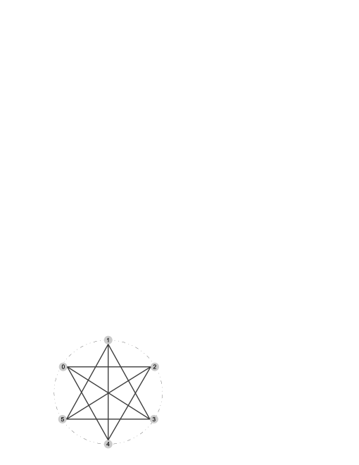
Figure 2: A translationally invariant graph state on the 1D torus ${\mathbb{T}}^{1}_{6}={\mathbb{Z}}_{6}$.

 

Figure 2 represents a translationally invariant graph state on the 1D torus ${\mathbb{T}}^{1}_{6}={\mathbb{Z}}_{6}$. The adjacency matrix $\Gamma$ is given by

$$\Gamma=\left(\begin{array}[]{cccccc}&&1&1&1&\\ &&&1&1&1\\ 1&&&&1&1\\ 1&1&&&&1\\ 1&1&1&&&\\ &1&1&1&&\end{array}\right)$$ (39)

and obviously only depends on the difference $x-y$ of the variables $x,y\in{\mathbb{Z}}_{6}$. Applying the Fourier transform, yields the polynomial $\hat{\gamma}=u^{2}+u^{3}+u^{4}=u^{-2}+u^{2}+u^{3}$. The symplectic cellular automaton, which creates the graph state as explained above is given by the matrix

$${\bf t}=\left(\begin{array}[]{cc}1&u^{-2}+u^{2}+u^{3}\\ 0&1\end{array}\right)\;.$$ (40)

Note that ${\bf t}$ is reflection invariant, since $\overline{{u^{3}}}=u^{3}$ is a reflection fix-point. $\lozenge$

We are going to present another example to show that the phase space vectors do not have to be reflection invariant, because not all invertible elements are monomials. But the invertibility of a fixed polynomial depends on the size of the torus and so a fixed phase space vector $\xi$ may define a translationally invariant stabilizer state for some $N$, but it is possible that there exists $N^{\prime}$, such that ${\mathcal{P}}_{1,N^{\prime}}\xi$ is not maximally isotropic, and therefore $\xi$ does not characterize a unique stabilizer state for $N^{\prime}$.

Example 4.4.

We consider for $p=2$ the phase space vector

$$\xi=(1+{u}+{u}^{3}){{u}^{-1}+{u}\choose 1}$$ (41)

on a one dimensional torus of variable size. Note that $\hat{\sigma}(\xi,\xi)=0$ holds for all $N$, so $\xi$ generates an isotropic subspace. The corresponding tensor product of Pauli operators is given by

$${\bf w}(\xi)=Z\otimes Y\otimes Y\otimes\openone\otimes X\otimes Z\;,$$ (42)

and is obviously not reflection invariant.

Let us first have a look at the case $N=7$. It is easy to show that $1+{u}+{u}^{3}$ is not invertible. We define $\tilde{\xi}=\xi/(1+{u}+{u}^{3})={{u}^{-1}+{u}\choose 1}$ and have that $\hat{\sigma}(\tilde{\xi},\xi)=0$, but $\tilde{\xi}\notin{\mathcal{P}}_{1,7}\xi$. So ${\mathcal{P}}_{1,7}\xi$ is not maximally isotropic, and there is no unique stabilizer state.

For $N=6$ the inverse of $1+{u}+{u}^{3}$ is given by ${u}+{u}^{4}+{u}^{5}$, so $\xi$ and $\tilde{\xi}$ generate the same subspace, which is actually maximally isotropic. So $\xi$ is indeed a valid column of a symplectic automaton, but starting from the “all spins up” state both CQCAs corresponding to

$${\bf t}=\left(\begin{array}[]{cc}{u}+{u}^{4}+{u}^{5}&(1+{u}+{u}^{3})({u}^{-1}+{u})\\ 0&(1+{u}+{u}^{3})\end{array}\right)\;,\quad\mbox{resp.}\quad\tilde{{\bf t}}=\left(\begin{array}[]{cc}1&{u}^{-1}+{u}\\ 0&1\end{array}\right)$$

prepare the same stabilizer state. $\lozenge$

5 Conclusions

We have analyzed the structure of Clifford quantum cellular automata that act on a $s$-dimensional lattice of $p$-level systems. The results which can be achieved depend on the dimension of the lattice and whether we put periodic boundary conditions or working with the infinite lattice.

We have characterized the group of CQCAs in terms of symplectic cellular automata on a suitable phase space. With the help of Fourier transform, this phase space can be identified with two-dimensional vectors of Laurent-polynomials, and symplectic cellular automata can be described by two-by-two matrices with Laurent-polynomial entries. We have shown that these entries must be reflection invariant and that up to some global shift the determinant of the matrix must be one, so the group of CQCAs is isomorphic to the special linear group of two-by-two matrices with reflection invariant polynomials as matrix elements.

We have proven that there is a correspondence between 1D CQCAs and 1D translationally invariant stabilizer states. For a fixed translationally invariant pure stabilizer state $\omega^{\otimes{\mathbb{Z}}}$, which is in particular a product state, every other translationally invariant pure stabilizer state $\varphi$ can be created by applying an appropriate CQCA $T_{\varphi}$ to the chosen product state: $\varphi=\omega^{\otimes{\mathbb{Z}}}\circ T_{\varphi}$.

Pure stabilizer states can be also characterized by maximally isotropic subspaces. We have characterized the phase space vectors, which generate maximally isotropic subspaces, namely their components must be coprime and reflection invariant.

In the one-dimensional case we have also more clarified the group structure of CQCAs. As we have shown, each one-dimensional CQCA can be decomposed into a product of elementary shear automata and local Fourier transforms, so the group of CQCAs is generated by this set of operations.

For periodic boundary conditions the techniques from infinitely extended lattices can be applied to a certain extend. According to the discussion of translationally invariant stabilizer states on the 1D lattice, we have proven that there is an analogous correspondence between CQCAs and translationally invariant stabilizer states with periodic boundary conditions even in any lattice dimension.

Appendix A Proofs and technicalities

A.1.  Ad Theorem 3.9

For the proof of Theorem 3.9 we need that a singly generated isotropic subspace can always be embedded into a singly generated maximally isotropic subspace:

Lemma A.1.

Let $0\neq\xi\in{\mathcal{P}}_{s}^{2}$ and ${\mathcal{P}}_{s}\xi$ be an isotropic, but not maximally isotropic ${\mathcal{P}}_{s}$-subspace. Then there exists a phase space vector $\eta\in{\mathcal{P}}_{s}^{2}$ such that ${\mathcal{P}}_{s}\eta\supsetneqq{\mathcal{P}}_{s}\xi$ is maximally isotropic.

Proof.

${\mathcal{P}}_{s}\xi$ is isotropic if and only if the equation $0=\hat{\sigma}(\xi,\xi)=\overline{{\xi}}_{+}\xi_{-}-\overline{{\xi}}_{-}\xi_{+}$ holds. We make a distinction of cases for this equation:

1. $\xi_{+}=0$ (analogously $\xi_{-}=0$): Then ${\mathcal{P}}_{s}\xi=\{0\}\oplus{\mathcal{P}}_{s}\xi_{-}$ and $\xi_{-}$ is not invertible since this would force ${\mathcal{P}}_{s}\xi=\{0\}\oplus{\mathcal{P}}_{s}$ to be maximally isotropic. So we can set $\eta=(0,1)$.

2. $\xi_{+}=f\xi_{-}$ (analogously $\xi_{-}=f\xi_{+}$) with $f$ reflection invariant: Then we have ${\mathcal{P}}_{s}\xi={\mathcal{P}}_{s}\xi_{-}(f,1)$. We set $\eta=(f,1)$ and get that ${\mathcal{P}}_{s}\eta$ is a maximally isotropic subspace since $0=\hat{\sigma}(\eta,\lambda)=f\lambda_{-}-\lambda_{+}$ implies $\lambda=\lambda_{-}\eta\in{\mathcal{P}}_{s}\eta$.

3. $\xi_{+}\neq 0\neq\xi_{-}$ and $\xi_{\pm}\neq f\xi_{\mp}$: Then $\xi=f\overline{{\xi}}$ with $f$ invertible, so $\xi$ is reflection invariant for some $n\in\frac{1}{2}{\mathbb{Z}}^{d}$. Because ${\mathcal{P}}_{s}\xi$ is not maximally isotropic we can find $\eta\notin{\mathcal{P}}_{s}\xi$ with $0=\hat{\sigma}(\xi,\eta)=u^{n}(\xi_{+}\eta_{-}-\xi_{-}\eta_{+})$. Since $\xi_{+}$ and $\xi_{-}$ are nonvanishing this implies $\xi=g\eta$ for some $g\in{\mathcal{P}}_{s}$. We can choose ${\rm gcd}(\eta_{+},\eta_{-})=1$ and ${\mathcal{P}}_{s}\eta$ to be maximally isotropic.

∎

A.2.  Ad Theorem 3.11

For a polynomial $f\in{\mathcal{P}}$ the coefficient of the monomial ${u}^{x}$ is $\langle{f}\rangle_{x}$. Recall that “degree”of a polynomial in $f\in{\mathcal{P}}$ is defined by ${\rm deg}({f}):=\max\{x|\langle{f}\rangle_{x}\not=0\}-\min\{x|\langle{f}\rangle_{x}\not=0\}$ and that the support is defined by ${\rm supp}(f):=\{x|\langle{f}\rangle_{x}\not=0\}$.

Lemma A.2.

Let $(\xi,\eta)$ be a symplectic cellular automaton which is invariant under the reflection at the origin: $\xi=\overline{{\xi}}$ and $\eta=\overline{{\eta}}$. If the degrees of column vectors fulfill ${\rm deg}({\xi})>{\rm deg}({\eta})$ then there exists a shear transformation ${{\bf g}({f})}$, with reflection invariant $f\in{\mathcal{P}}$, such that the symplectic transformation

$$(\xi^{\prime},\eta^{\prime})=(\xi,\eta){{\bf g}({f})}{\bf f}_{1}$$ (43)

satisfies ${\rm deg}({\xi,\eta})>{\rm deg}({\xi^{\prime},\eta^{\prime}})$ and ${\rm deg}({\xi^{\prime}})>{\rm deg}({\eta^{\prime}})$.

Proof.

Since $\xi$ and $\eta$ are reflection invariant, the degree is an even integer and we introduce $x:={\rm deg}({\xi})/2$, $y:={\rm deg}({\eta})/2$, as well as $n_{1}:=x-y>0$. We conclude from the identity $\hat{\sigma}(\xi,\eta)=1$ that

$$\langle{\hat{\sigma}(\xi,\eta)}\rangle_{x+y}=\langle{\xi_{+}}\rangle_{-x}\langle{\eta_{-}}\rangle_{y}-\langle{\xi_{-}}\rangle_{-x}\langle{\eta_{+}}\rangle_{y}=0$$ (44)

is valid. This implies that

$$\langle{\xi}\rangle_{x}=\langle{\xi}\rangle_{-x}=-f_{1}\langle{\eta}\rangle_{y}=-f_{1}\langle{\eta}\rangle_{-y}$$ (45)

for some $f_{1}\in{\mathbb{F}}$. Now $\langle{\xi+f_{1}({u}^{n_{1}}+{u}^{-{n_{1}}})\eta}\rangle_{\pm x}=0$ which implies that

$${\rm deg}({\xi+f_{1}({u}^{n_{1}}+{u}^{-{n_{1}}})\eta})<{\rm deg}({\xi})\;.$$ (46)

Now we observe

$$(\xi_{1},\eta_{1}) := (\xi,\eta){{\bf g}({f_{1}({u}^{n_{1}}+{u}^{-{n_{1}}})})}$$ (51)

$$= \left(\begin{array}[]{cc}\xi_{+}&\eta_{+}\\ \xi_{-}&\eta_{-}\end{array}\right){\left(\begin{array}[]{cc}1&0\\ {f_{1}({u}^{n_{1}}+{u}^{-{n_{1}}})}&1\end{array}\right)}$$

$$= \left(\begin{array}[]{cc}\xi_{+}+f_{1}({u}^{n_{1}}+{u}^{-{n_{1}}})\eta_{+}&\eta_{+}\\ \xi_{-}+f_{1}({u}^{n_{1}}+{u}^{-{n_{1}}})\eta_{-}&\eta_{-}\end{array}\right)$$ (54)

from which we conclude that ${\rm deg}({\xi_{1},\eta_{1}})<{\rm deg}({\xi,\eta})$. If ${\rm deg}({\xi_{1}})>{\rm deg}({\eta_{1}})$ we can find a shear transformation ${{\bf g}({f_{2}({u}^{n_{2}}+{u}^{-{n_{2}}})})}$ such that

$$(\xi_{2},\eta_{2})=(\xi_{1},\eta_{1}){{\bf g}({f_{2}({u}^{n_{2}}+{u}^{-{n_{2}}})})}$$ (55)

fulfills ${\rm deg}({\xi_{2},\eta_{2}})<{\rm deg}({\xi_{1},\eta_{1}})$. We can proceed this reduction until the $l$th step with $2l=|{\rm supp}(\xi)\setminus{\rm supp}(\eta)|$. The resulting symplectic cellular automaton

$$(\xi_{l},\eta_{l})=(\xi_{l-1},\eta_{l-1}){{\bf g}({f_{l}({u}^{n_{l}}+{u}^{-{n_{l}}})})}$$ (56)

then satisfies ${\rm deg}({\xi_{l}})\leq{\rm deg}({\eta_{l}})$. If ${\rm deg}({\xi_{l}})={\rm deg}({\eta_{l}})$ then, there is an appropriate constant $f_{l+1}\in{\mathbb{F}}$ such that

$$(\xi^{\prime},\eta^{\prime})=(\xi,\eta){{\bf g}({f})}{\bf f}_{1}=(-\eta_{l},\xi_{l}+f_{l+1}\eta_{l})$$ (57)

holds with ${\rm deg}({\xi^{\prime}})>{\rm deg}({\eta^{\prime}})$. Here $f$ is the reflection invariant polynomial

$$f=\sum_{j=1}^{l+1}f_{j}({u}^{n_{j}}+{u}^{-{n_{j}}})\;.$$ (58)

If ${\rm deg}({\xi_{l}})<{\rm deg}({\eta_{l}})$, then the shear transformation ${{\bf g}({f_{l+1}})}$ is not applied and we get

$$(\xi^{\prime},\eta^{\prime})=(\xi,\eta){{\bf g}({f})}{\bf f}_{1}=(-\eta_{l},\xi_{l})$$ (59)

with the polynomial $f=\sum_{j=1}^{l}f_{j}({u}^{n_{j}}+{u}^{-{n_{j}}})$. ∎

Proof of Theorem 3.11..

Let $(\xi_{0},\eta_{0})$ be a symplectic cellular automaton which is invariant under the reflection at the origin. Then, by Lemma A.2, there exists a symplectic cellular automaton $(\xi_{1},\eta_{1})$ and a shear transformation ${{\bf g}({f_{1}})}$ such that

$$(\xi_{0},\eta_{0})=(\xi_{1},\eta_{1}){{\bf g}({f_{1}})}{\bf f}_{1}$$ (60)

and ${\rm deg}({\xi_{1}})>{\rm deg}({\eta_{1}})$. Thus we can iterate this reduction process until $(\xi_{k},\eta_{k})$ is a constant symplectic transformation (corresponding to a QCA with single cell neighborhood), which can be decomposed into a product of local shear transformations ${{\bf g}({{w_{0}}})}$ and local Fourier transforms ${\bf f}_{c_{i}}$ with $c_{i}\in{\mathbb{F}}$. This yields the following decomposition of $(\xi_{0},\eta_{0})$:

$$(\xi_{0},\eta_{0})={{\bf g}({f_{r}})}{\bf f}_{c_{r}}\cdots{{\bf g}({f_{2}})}{\bf f}_{c_{2}}{{\bf g}({f_{1}})}{\bf f}_{c_{1}}\;.$$ (61)

∎

References

- [1] Conway, J. H.: On numbers and games, Academic Press, London (1976). Second edition: A. K. Peters, Wellesley/MA (2001).
- [2] Schumacher, B. and Werner, R. F.: Reversible quantum cellular automata, quant-ph/0405175
- [3] Krüger, O. and Werner, R. F.: Gaussian Quantum Cellular Automata, In: N. Cerf, G. Leuchs, E.S. Polzik (ed.), ”Quantum Information with continuous variables of atoms and light”, Imperial College Press (2007).
- [4] Feynman, R.: Simulating physics with computers, Int. J. Theor. Phys. 21, 467-488, (1982)
- [5] Raussendorf, R. and Briegel, H.-J.: Computational model underlying the one-way quantum computer, Quant. Inf. Comp. 2, No.6, 443-486 (2002)
- [6] Bratteli, O. and Robinson, D.: Operator algebras and quantum statistical mechanics. Volume I & II, Spinger-Verlag (1979)
- [7] Scutaru, H.: Some remarks on covariant completely positive maps, Rep. Math. Phys. 16 79-87 (1979)
- [8] Holevo, A. S.: Remarks on the classical capacity of quantum channel, quant-ph/0212025
- [9] Holevo, A. S.: Additivity conjecture and covariant channels, Proc. Conference ”Foundations of Quantum Information”, Camerino (2004)
- [10] Jacobson, N.: Lectures in abstract algebra. Volume I: Basic Concepts, Graduate Texts in Mathematics, No. 30., Springer-Verlag, New York-Berlin (1975)
- [11] Gottesman, D.: The Heisenberg representation of quantum computers, Published in Hobart 1998, Group theoretical methods in physics 32-43, quant-ph/9807006.
- [12] Bernstein, E. and Vazirani, U.: Quantum complexity theory, Proc. 25th Ann. ACM Symp. on Theory of Computing, 11-20 (1993)
- [13] Watrous, J.: On one-dimensional quantum cellular automata, Proc. 36th Ann. Symp. on Foundations of Computer Science, 528-537 (1995)
- [14] Zmud, E. M.: Symplectic geometry and projective representations of finite abelian groups, Math. USSR Sbornik, 16, 1-16 (1972)
- [15] Gottesman, D.: Stabilizer Codes and Quantum Error Correction, Ph.D. thesis, Caltech, quant-ph/9705052 (1997)
- [16] Nielsen, M. A. and Chuang, I. L.: Quantum Computation and Quantum Information, Cambridge University Press (2000)
- [17] Schlingemann, D.-M.: Cluster states, graphs and algorithms. Quant. Inf. Comp. 4 (4) (2004) 287-324
- [18] Daubechies, I. and Sweldens, W.: Factoring Wavelet transforms into lifting steps, J. Four. Anal. Appl. 4(3) (1998)
- [19] Brown, W. S.: On Euclid’s Algorithm and the Computation of Polynomial Greatest Common Divisors, J. Assoc. Comp. Mach., Vol. 18, No. 4, pp. 478-504 (1971)
- [20] McDuff, D. and Salamon, D.: Introduction to Symplectic Topology, Oxford Mathematical Monographs (1998)