Nanowire waveguide made from extremely anisotropic metamaterials

Abstract

Exact solutions are obtained for all the modes of wave propagation along an anisotropic cylindrical waveguide. Closed-form expressions for the energy flow on the waveguide are also derived. For extremely anisotropic waveguide where the transverse permittivity is negative ($\varepsilon_{\bot}<0$) while the longitudinal permittivity is positive ($\varepsilon_{||}>0$), only transverse magnetic (TM) and hybrid modes will propagate on the waveguide. At any given frequency the waveguide supports an infinite number of eigenmodes. Among the TM modes, at most only one mode is forward wave. The rest of them are backward waves which can have very large effective index. At a critical radius, the waveguide supports degenerate forward- and backward-wave modes with zero group velocity. These waveguides can be used as phase shifters and filters, and as optical buffers to slow down and trap light.

I Introduction

Since the realization of negative refraction Veselago in microwaves Shelby , there is renewed and intense interest in electromagnetic metamaterials. Negative refraction has added a new arena to physics, leading to new concepts such as perfect lens Pendry00 ; Lu05 , superlens Pendry00 ; Lu03 ; Fang , and focusing by plano-concave lens Vodo05 ; Vodo06 . Negative refraction has subsequently been realized in microwaves Parazzoli ; Parimi04 ; Parimi03 ; Cubukcu ; LuZ , THz waves, and optical wavelengths Berrier ; Dolling ; Soukoulis07 , in metamaterials made of wire and split-ring resonators Smith04 or photonic crystals Notomi ; Gralak ; Luo02 .

Metamaterials are artifically fabricated structures possessing certain desirable properties which are not available in natural materials. Metamaterials can have double negative index Shalaev or single negative index. Metamaterials can be periodic, such as photonic crystals Joannopoulos . They can also be non-periodic, such as the materials for cloaking Schurig06 . They can also be made to be anisotropic and have indefinite index Smith03 ; Hoffman ; Lu07 . Indefinite index matematerials can be used to make hyperlens LiuZ ; Smolyaninov . This range of properties opens an infinite possibilities to use matematerials in frequencies from microwave all the way up to the visible.

Wave propagation in waveguide of nanometer size Takahara has unique properties. In this paper, we consider wave propagation along anisotropic nanowires. In the case where the transverse permittivity is negative while the longitudinal one is positive ($\varepsilon_{\bot}<0$, $\varepsilon_{||}>0$), these indefinite index waveguides can support both forward and backward waves. High effective index can be obtained for these modes. These waveguides can also support degenerate modes which can be used to slow down and trap light.

In Sec. II, we derive the formulas for all the modes on the anisotropic cylinders. Exact solutions for all the modes and closed-form expressions for the energy flow will be obtained. Possible zero net-energy flow modes will also be discussed. The situation for trapping light is presented in Sec. III. In Sec. IV, we propose the realization of nanowires made of indefinite index medium, which is confirmed in finite-difference time-domain simulations. We conclude in Sec. V with possible applications for these anisotropic nanowires.

II Wave propagation and energy flow on anisotropic cylindrical waveguides

We consider wave propagation on a cylindrical waveguide. The axis of the waveguide is along the $z$-direction as shown in Fig. 1. The waveguide is nonmagnetic and has an anisotropic optical property

$$\varepsilon_{x}=\varepsilon_{y}=\varepsilon_{t}\neq\varepsilon_{z}.$$ (1)

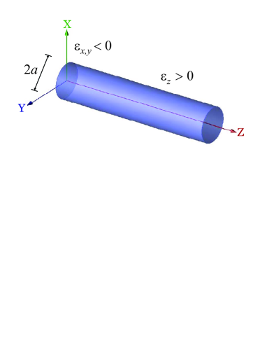
Figure 1: (Color online) An anisotropic cylindrical waveguide with axis along the $z$-axis. The longitudinal permittivity is positive while the transverse permittivity is negative.

The waves will propagation along the cylinder axis with

$${\bf E}={\bf E}_{0}e^{i(\beta z-\omega t)},\quad{\bf H}={\bf H}_{0}e^{i(\beta z-\omega t)}.$$ (2)

Here $\beta$ is the propagation wave number along the waveguide.

Due to the symmetry of the waveguide, all the field components can be expressed in terms of the longitudinal components $E_{z}$ and $H_{z}$. In the polar coordinate system, one has for the fields inside the waveguide $r<a$ with $a$ the radius,

$$E_{r} = i{1\over\varepsilon_{t}k_{0}^{2}-\beta^{2}}\Big{(}\beta\partial_{r}E_{z}+k_{0}{1\over r}\partial_{\phi}H_{z}\Big{)},$$

$$E_{\phi} = i{1\over\varepsilon_{t}k_{0}^{2}-\beta^{2}}\Big{(}\beta{1\over r}\partial_{\phi}E_{z}-k_{0}\partial_{r}H_{z}\Big{)},$$

$$H_{r} = i{1\over\varepsilon_{t}k_{0}^{2}-\beta^{2}}\Big{(}-\varepsilon_{t}k_{0}{1\over r}\partial_{\phi}E_{z}+\beta\partial_{r}H_{z}\Big{)},$$

$$H_{\phi} = i{1\over\varepsilon_{t}k_{0}^{2}-\beta^{2}}\Big{(}\varepsilon_{t}k_{0}\partial_{r}E_{z}+\beta{1\over r}\partial_{\phi}H_{z}\Big{)}.$$ (3)

Here $k_{0}$ is the wave number in the vacuum.

The wave equations for the longitudinal components inside the waveguide are

$$(\partial^{2}_{x}+\partial^{2}_{y})E_{z}+\varepsilon_{z}(k_{0}^{2}-\beta^{2}/\varepsilon_{t})E_{z}=0,$$

$$(\partial^{2}_{x}+\partial^{2}_{y})H_{z}+(\varepsilon_{t}k_{0}^{2}-\beta^{2})H_{z}=0.$$ (4)

The waveguide is free-standing in air, so the wave equations for $r>a$ are given by the above equations with the permittivity replaced by unity. The solutions are expressed in terms of the Bessel functions of various kinds

$$E_{z} = AJ_{n}(Kr)e^{in\phi},\ \quad r<a,$$ (5)

$$= CK_{n}(\kappa_{0}r)e^{in\phi},\quad r>a$$

and

$$H_{z} = BI_{n}(\kappa r)e^{in\phi},\qquad r<a,$$ (6)

$$= DK_{n}(\kappa_{0}r)e^{in\phi},\quad r>a.$$

The coefficients will be determined by matching the boundary conditions. Here

$$K = \sqrt{\varepsilon_{z}}\sqrt{k_{0}^{2}-\beta^{2}/\varepsilon_{t}},$$

$$\kappa = \sqrt{\beta^{2}-\varepsilon_{t}k_{0}^{2}},$$

$$\kappa_{0} = \sqrt{\beta^{2}-k_{0}^{2}}.$$ (7)

We only consider the extremely anisotropic case such that the longitudinal permittivity is positive while the transverse permittivity is negative

$$\varepsilon_{z}>0,\quad\varepsilon_{t}<0.$$ (8)

One can see that due to the anisotropic nature of the waveguide, $H_{z}$ and $E_{z}$ inside the waveguide will have completely different behaviors.

The continuity of $E_{z}$ and $H_{z}$ at the interface $r=a$ gives

$${C\over A}={J_{n}(Ka)\over K_{n}(\kappa_{0}a)},\quad{D\over B}={I_{n}(\kappa a)\over K_{n}(\kappa_{0}a)}.$$ (9)

The continuity of $E_{\phi}$ at the interface gives

$$in\beta{\kappa_{0}^{2}-\kappa^{2}\over k_{0}a^{2}\kappa_{0}^{2}\kappa^{2}}={B\over A}{I_{n}(\kappa a)\over J_{n}(Ka)}\Big{[}g_{n}(\kappa_{0}a)+h_{n}(\kappa a)\Big{]}$$ (10)

with the following defined functions

$$g_{n}(x) = -{K^{\prime}_{n}(x)\over xK_{n}(x)}={K_{n-1}(x)\over xK_{n}(x)}+{n\over x^{2}},$$

$$h_{n}(x) = {I^{\prime}_{n}(x)\over xI_{n}(x)}={I_{n-1}(x)\over xI_{n}(x)}-{n\over x^{2}}.$$ (11)

The continuity of $H_{\phi}$ at the interface gives

$$in\beta{\kappa^{2}-\kappa_{0}^{2}\over k_{0}a^{2}\kappa_{0}^{2}\kappa^{2}}={A\over B}{J_{n}(Ka)\over I_{n}(\kappa a)}\Big{[}g_{n}(\kappa_{0}a)-\varepsilon_{z}f_{n}(Ka)\Big{]}$$ (12)

with

$$f_{n}(x)={J^{\prime}_{n}(x)\over xJ_{n}(x)}={J_{n-1}(x)\over xJ_{n}(x)}-{n\over x^{2}}.$$ (13)

Thus we obtain the equation for all the modes

$$\Big{[}g_{n}(\kappa_{0}a)-\varepsilon_{z}f_{n}(Ka)\Big{]}\Big{[}g_{n}(\kappa_{0}a)+h_{n}(\kappa a)\Big{]}$$

$$=n^{2}\Big{[}(\kappa_{0}a)^{-2}-(\kappa a)^{-2}\Big{]}\Big{[}(\kappa_{0}a)^{-2}-\varepsilon_{t}(\kappa a)^{-2}\Big{]}.$$ (14)

For wave propagation on the cylindrical waveguide, the components of the Poynting vector are

$$S_{z} = {1\over 4\pi}(E_{r}H_{\phi}^{*}-E_{\phi}H_{r}^{*}),$$

$$S_{r} = -{1\over 4\pi}(E_{z}H_{\phi}^{*}-E_{\phi}H_{z}^{*}),$$

$$S_{\phi} = {1\over 4\pi}(E_{z}H_{r}^{*}-E_{r}H_{z}^{*}).$$ (15)

The physical Poynting vector is given by $\Re{\bf S}$.

The total energy flow along the waveguide is the sum of energy flow inside and outside the waveguide

$$P_{z}=P^{\rm in}_{z}+P^{\rm out}_{z}$$ (16)

with

$$P^{\rm in}_{z}=2\pi\int_{0}^{a}S_{z}rdr,\quad P^{\rm out}_{z}=2\pi\int_{a}^{\infty}S_{z}rdr.$$ (17)

Following Ref. Tsakmakidis06 , the total energy flow is normalized as

$$\langle P_{z}\rangle={P^{\rm in}_{z}+P^{\rm out}_{z}\over|P^{\rm in}_{z}|+|P^{\rm out}_{z}|}.$$ (18)

Thus one has $-1<\langle P_{z}\rangle<1$.

In the following, we discuss different modes in detail.

II.1 TE modes

For the transverse electric (TE) modes, $E_{z}=0$. The longitudinal magnetic field is given by Eq. (6). One has

$$E_{\phi} = i{k_{0}\over\kappa^{2}}\partial_{r}H_{z}=i{k_{0}\over\kappa}BI_{1}(\kappa r),\qquad r<a,$$ (19)

$$= i{k_{0}\over\kappa_{0}^{2}}\partial_{r}H_{z}=-i{k_{0}\over\kappa_{0}}DK_{1}(\kappa r),\quad r>a.$$

The continuity of $E_{\phi}$ at the interface requires that

$$h_{0}(\kappa a)+g_{0}(\kappa_{0}a)=0.$$ (20)

For materials without loss, each term on the left side is positive, thus there is no solution. The waveguide does not support TE modes. This is exactly like that of a metallic wire which does not support TE surface waves since current must flow along the waveguide.

Only when $\varepsilon_{t}>1$, the waveguide will support TE modes, like an ordinary dielectric fiber.

II.2 TM modes

For the transverse magnetic (TM) modes, $H_{z}=0$. The longitudinal electric field is given by Eq. (5). One has

$$H_{\phi} = -i\varepsilon_{z}{k_{0}\over K}AJ_{1}(Kr),\quad r<a,$$ (21)

$$= i{k_{0}\over\kappa_{0}}CK_{1}(\kappa_{0}r),\qquad r>a.$$

The continuity of $H_{\phi}$ leads to the equation

$$\varepsilon_{z}f_{0}(Ka)=g_{0}(\kappa_{0}a).$$ (22)

The solutions to this equation give all the TM modes.

II.2.1 Band structure of TM modes

We first consider the solutions for fixed and real values of $\varepsilon_{z}$ and $\varepsilon_{t}$. This is normally associated with a fixed $k_{0}$. It is convenient to consider solution in the form of $Ka$ or the reduced radius $k_{0}a$ as a function of $\kappa_{0}a$. The wave number along the waveguide can be obtained through $\beta=(k_{0}^{2}+\kappa_{0}^{2})^{1/2}$. Before we seek general solutions, it is better to consider the solutions in certain limits to reveal some important features of the TM modes on the anisotropic waveguide.

For the TM modes close to the light line, $\kappa_{0}a\to 0$, one has

$$Ka\simeq x_{0,m}-{\varepsilon_{z}\over x_{0,m}}(\kappa_{0}a)^{2}(\ln{\kappa_{0}a\over 2}+\gamma).$$

Here we have used $K_{0}(x)=-\ln(x/2)-\gamma$ for small augument with $\gamma$ the Euler constant. For complex $\varepsilon_{t}$ with $\Re\varepsilon_{t}<0$ and $\Im\varepsilon_{t}>0$, the real and imaginary parts of $\beta$ of the allowed modes will have the same signs. These modes are forward waves, similar to that of an ordinary optical fiber. We note that close to the light line, the property of the TM modes of the anisotropic waveguide is similar to that of an isotropic fiber with $\varepsilon=1+\varepsilon_{z}(1-\varepsilon_{t}^{-1})$.

In the limit of long wavelength or small waveguide radius, $k_{0}a\ll 1$, Eq. (22) is reduced to

$$\varepsilon_{z}f_{0}(\kappa_{0}a/\eta)=g_{0}(\kappa_{0}a)$$ (23)

with $\eta=\sqrt{-\varepsilon_{t}/\varepsilon_{z}}$. This equation gives an infinite number of solutions $\kappa_{0}a=\xi_{0,m}$ with $m=1,2,3,\cdots$. This indicates that the anisotropic waveguide supports infinite number of propagating modes, no matter how thin the waveguide is. For $\kappa_{0}a\to\infty$, since $g_{0}(\kappa_{0}a)\simeq(\kappa_{0}a)^{-1}\to 0$, one has $\xi_{m}\simeq\eta x_{1,m}$. Here $x_{n,m}$ is the $m$-th zero of $J_{n}(x)$ away from the origin. For the $m$-th TM band, one has $0\leq\kappa_{0}a\leq\xi_{0,m}$. The $m$-th band starts with $k_{0}a=x_{0,m}/\sqrt{\varepsilon_{z}-\varepsilon_{z}/\varepsilon_{t}}$ when $\kappa_{0}a=0$ and ends at $k_{0}a=0$ when $\kappa_{0}a=\xi_{0,m}$. The modes with $\kappa_{0}\gg k_{0}$ have $d(k_{0}a)/d(\kappa_{0}a)<0$ and are backward wave. It will be obvious if we include small imaginary part in $\varepsilon_{t}$ with $\Im\varepsilon_{t}>0$. The equation will give $\beta$ with the real and imaginary parts having opposite signs. The energy flow is opposite to the phase velocity, which will be discussed later.

For arbitrary values of $\kappa_{0}a$, the solution must be sought numerically. Since the right-hand side of Eq. (22) is always positive, the solution requires that $J_{1}(Ka)$ and $J_{0}(Ka)$ have different signs. For the $m$-th band, since $0\leq\kappa_{0}a\leq\xi_{0,m}$ with $\xi_{0,m}$ the solutions of Eq. (23), one has $x_{0,m}\leq Ka\leq\xi_{0,m}/\eta<x_{1,m}$. For each $\kappa_{0}a$ value, the $Ka$ value can be searched within $[x_{0,m},x_{1,m}]$ to satisfy Eq. (22). Once the corresponding $Ka$ is found, the reduced radius can be obtained as

$$k_{0}a={\sqrt{(-\varepsilon_{t}/\varepsilon_{z})(Ka)^{2}-(\kappa_{0}a)^{2}}\over\sqrt{1-\varepsilon_{t}}}.$$

For the $m$-th band, the corresponding transverse electric field $E_{z}$ will have $m$ nodes. The band structure for a waveguide with $\varepsilon_{t}=-3$ and $\varepsilon_{z}=2$ is shown in Fig. 2. The effective index of the waveguide $n_{\rm eff}\equiv\beta/k_{0}$ is also evaluated and plotted in Fig. 3.

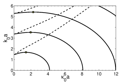
Figure 2: Band structure of the guided TM modes on an anisotropic waveguide of radius $a$ with $\varepsilon_{t}=-3$ and $\varepsilon_{z}=2$. Open circles denote the degenerate points of forward-wave and backward-wave modes. The dashed lines are for a dielectric waveguide with $\varepsilon=1+\varepsilon_{z}(1-\varepsilon_{t}^{-1})$.

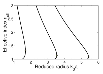
Figure 3: Effective index $n_{\rm eff}$ as a function of the reduced radius $k_{0}a$ for the first three bands of TM modes on an anisotropic waveguide with $\varepsilon_{t}=-3$ and $\varepsilon_{z}=2$. Open circles denote the degenerate points of forward-wave and backward-wave modes.

Unlike an ordinary fiber where for each band, $d(k_{0}a)/d(\kappa_{0}a)>0$, each TM band of the anisotropic waveguide starts with $d(k_{0}a)/d(\kappa_{0}a)>0$ for small $\kappa_{0}a$ or near the light line. At certain value of $\kappa_{0}a$ or $k_{0}a$ which is marked in Fig. 2, $d(k_{0}a)/d(\kappa_{0}a)=0$. Further increasing $\kappa_{0}a$ results in $d(k_{0}a)/d(\kappa_{0}a)<0$. The band ends at a finite $\kappa_{0}a=\xi_{0,m}$. Immediately below the point $k_{0}a$ where $d(k_{0}a)/d(\kappa_{0}a)=0$, each band has two modes with opposite signs of $d(k_{0}a)/d(\kappa_{0}a)$. One mode is forward wave and the other backward wave. This will be discussed later in the paper.

We next consider a waveguide of a fixed radius $a$ with the following permittivity

$$\varepsilon_{t} = {1\over 2}(1+\varepsilon_{a}-k_{p}^{2}/k_{0}^{2}),$$

$$\varepsilon_{z} = 2\varepsilon_{a}(k_{0}^{2}-k_{p}^{2})/[k_{0}^{2}(1+\varepsilon_{a})-k_{p}^{2}].$$ (24)

Here $\varepsilon_{a}$ and $k_{p}$ are positive constants. The realization of this property will be discussed later in Sec. IV. If $k_{0}<k_{p}/(1+\varepsilon_{a})^{1/2}$, one has $\varepsilon_{t}<0$ and $\varepsilon_{z}>0$. The band structure of the TM modes on this waveguide is obtained by numeric means and plotted in Fig. 4 with the corresponding effective index in Fig. 5. For this waveguide, there is no cutoff of $\kappa_{0}a$ for each band. This is because that as $k_{0}\to 0$, $\varepsilon_{z}\simeq 2\varepsilon_{a}$ and $\varepsilon_{t}\to-\infty$, thus $\eta=\sqrt{-\varepsilon_{t}/\varepsilon_{z}}\to\infty$. The cutoff $\xi_{0,m}\simeq\eta x_{1,m}\to\infty$.

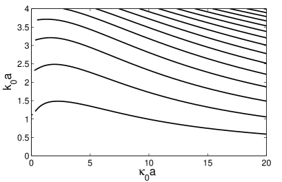
Figure 4: Band structure of the guided TM modes on an anisotropic waveguide of radius $a$ with $\varepsilon_{t}$ and $\varepsilon_{z}$ given by Eq. (24) with $a=10/k_{p}$ and $\varepsilon_{a}=2.25$.

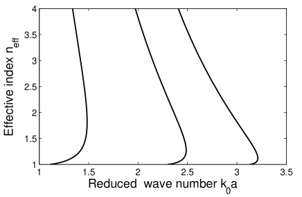
Figure 5: Effective index $n_{\rm eff}$ as a function of the reduced wave number $k_{0}a$ for the first three bands of TM modes on an anisotropic waveguide with $\varepsilon_{t}$ and $\varepsilon_{z}$ given by Eq. (24) with $a=10/k_{p}$ and $\varepsilon_{a}=2.25$.

We point out that the Padé approximant for the function $f_{0}(x)\equiv-x^{-1}J_{1}(x)/J_{0}(x)$ can be used to obtain good estimate of the solutions. This will be discussed in the Appendix.

If $\varepsilon_{t}>0$ and $\varepsilon_{z}<0$, the waveguide also supports TM modes. The details will not be presented here.

II.2.2 Energy flow of TM modes

Within the waveguide, one has $E_{z}=AJ_{0}(Kr)$, $E_{r}=i(\varepsilon_{z}\beta/\varepsilon_{t}K)AJ_{1}(Kr)$, and $H_{\phi}=i(\varepsilon_{z}k_{0}/K)AJ_{1}(Kr)$. So the Poynting vector component along the axis of the waveguide is

$$S_{z}={\beta\over\varepsilon_{t}k_{0}a^{2}}\Big{|}{J_{1}(Kr)\over J_{1}(Ka)}\Big{|}^{2}.$$ (25)

Here we set the coefficient $A=K/[\varepsilon_{z}k_{0}aJ_{1}(Ka)]$. Since $\varepsilon_{t}<0$, the energy flow inside the nanowire is always opposite to the phase velocity.

For the field in the air $r>a$, one has $E_{z}=CK_{0}(\kappa_{0}r)$, $E_{r}=i(\beta\/\kappa_{0})CK_{1}(\kappa_{0}r)$, and $H_{\phi}=i(k_{0}/\kappa_{0})CK_{1}(\kappa_{0}r)$, thus

$$S_{z}={\beta\over k_{0}a^{2}}\Big{|}{K_{1}(\kappa_{0}r)\over K_{1}(\kappa_{0}a)}\Big{|}^{2}.$$ (26)

Here the coefficient $C=-\kappa_{0}/[k_{0}aK_{1}(\kappa_{0}a)]$.

For the TM modes, one has

$$P^{\rm in}_{z} = {\beta\over 2\varepsilon_{t}k_{0}a^{2}}\int_{0}^{a}\Big{|}{J_{1}(Kr)\over J_{1}(Ka)}\Big{|}^{2}rdr,$$

$$P^{\rm out}_{z} = {\beta\over 2k_{0}a^{2}}\int_{a}^{\infty}\Big{|}{K_{1}(\kappa_{0}r)\over K_{1}(\kappa_{0}a)}\Big{|}^{2}rdr.$$ (27)

The above integrals can be carried out and more compact expressions for the energy flow can be obtained as

$$P^{\rm in}_{z} = {\beta\over 4\varepsilon_{t}k_{0}(Ka)^{2}}\Big{[}{1\over f_{0}^{2}(Ka)}+{2\over f_{0}(Ka)}+(Ka)^{2}\Big{]}$$

$$= -{\beta\over 4k_{0}\varepsilon_{z}^{2}f^{2}_{0}(Ka)}{\varepsilon_{z}^{2}f^{\prime}_{0}(Ka)\over\varepsilon_{t}Ka},$$

$$P^{\rm out}_{z} = {\beta\over 4k_{0}(\kappa_{0}a)^{2}}\Big{[}{1\over g_{0}^{2}(\kappa_{0}a)}+{2\over g_{0}(\kappa_{0}a)}-(\kappa_{0}a)^{2}\Big{]}$$ (28)

$$= -{\beta\over 4k_{0}g_{0}^{2}(\kappa_{0}a)}{g^{\prime}_{0}(\kappa_{0}a)\over\kappa_{0}a}.$$

Here $g^{\prime}_{0}(x)$ and $f^{\prime}_{0}(x)$ are the derivatives of $g_{0}(x)$ and $f_{0}(x)$, respectively.

For convenience, we set $\beta>0$ throughout the paper. Since $g^{\prime}_{0}(x)<0$ and $f^{\prime}_{0}(x)<0$, one has $P^{\rm in}_{z}<0$ and $P^{\rm out}_{z}>0$. In this convention, if $\langle P_{z}\rangle>0$, this indicates that the energy flow and the phase propagation are in the same directions and the mode is a forward-wave mode. Otherwise $\langle P_{z}\rangle<0$, the group velocity and the phase velocity are in the opposite direction and the mode is a backward-wave mode. The normalized energy flow for TM modes on a waveguide with $\varepsilon_{t}=-3$ and $\varepsilon_{z}=2$ is shown in Fig. 6. We note that for some portion of the bands the value of $\langle P_{z}\rangle$ is negative and thus these modes are backward waves.

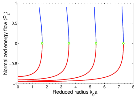
Figure 6: (Color online) Normalized energy flow $\langle P_{z}\rangle$ for the first four bands of the TM modes on an anisotropic waveguide with $\varepsilon_{t}=-3$ and $\varepsilon_{z}=2$. Here we set $\beta>0$. Open circles denote the degenerate points where $\langle P_{z}\rangle=0$.

II.2.3 Forward-wave and backward-wave TM modes

There are three ways to determine whether a mode is a forward wave or backward wave. One is through the sign of the derivative $d(k_{0}a)/d(\kappa_{0}a)$. From the band structure, we have already notice that for the modes near the light line, $d(k_{0}a)/d(\kappa_{0}a)>0$. These modes are forward waves. For large $\kappa_{0}a$ or small $k_{0}a$, one has $d(k_{0}a)/d(\kappa_{0}a)<0$, these modes are backward waves. From the band structure shown in Fig. 2, the majority of the modes are backward waves.

The second way is through the sign of $\langle P_{z}\rangle$. For the TM modes when $\kappa_{0}a\to\infty$, one has $f_{0}(Ka)\to 0$ since $g_{0}(\kappa_{0}a)\to 0$. One thus has $Ka\to x_{0,m}$. This solution leads to the divergence of $P^{\rm in}_{z}$ which is negative and the vanishing of $P^{\rm out}_{z}$ which is positive, subsequently $\langle P_{z}\rangle\to-1$, these modes are all backward waves. Correspondingly, one has $d(k_{0}a)/d(\kappa_{0}a)\to-\infty$ for $\kappa_{0}a\to\infty$. This is evident from the band structure shown in Fig. 2.

In the following, we prove that $d(k_{0}a)/d(\kappa_{0}a)\geq 0$ leads to $\langle P_{z}\rangle\geq 0$ and vice versa. We consider the derivative

$${d(Ka)\over d(\kappa_{0}a)}=-{\varepsilon_{z}\over\varepsilon_{t}Ka}\Big{[}\kappa_{0}a+(1-\varepsilon_{t})k_{0}a{d(k_{0}a)\over d(\kappa_{0}a)}\Big{]}.$$

Thus one has

$$\quad{d(Ka)\over d(\kappa_{0}a)}+{\varepsilon_{z}\kappa_{0}a\over\varepsilon_{t}Ka}\geq 0\quad{\rm if}\quad{d(k_{0}a)\over d(\kappa_{0}a)}\geq 0.$$

On the other hand, according to the eigen equation $\varepsilon_{z}f_{0}(Ka)=g_{0}(\kappa_{0}a)$, one has

$${d(Ka)\over d(\kappa_{0}a)}={g^{\prime}_{0}(\kappa_{0}a)\over\varepsilon_{z}f^{\prime}_{0}(Ka)}.$$

Making use of the above expression, one arrives at the inequality

$$-{\varepsilon_{z}^{2}f^{\prime}_{0}(Ka)\over\varepsilon_{t}Ka}-{g^{\prime}_{0}(\kappa_{0}a)\over\kappa_{0}a}\geq 0,$$

and subsequently

$$P^{\rm in}_{z}+P^{\rm out}_{z}\geq 0,\quad{\rm if}\quad{d(k_{0}a)\over d(\kappa_{0}a)}\geq 0.$$ (29)

Similarly one has

$$P^{\rm in}_{z}+P^{\rm out}_{z}\leq 0\quad{\rm if}\quad{d(k_{0}a)\over d(\kappa_{0}a)}\leq 0.$$ (30)

So the condition for $P_{z}=0$ can be allocated from the band structures as shown in Fig. 2, 4 when $d(k_{0}a)/d(\kappa_{0}a)=0$.

The third way to determine whether a mode is a forward or backward wave is through the relative sign of the real and imaginary parts of $\beta$ if dissipation is included. For example we consider $\varepsilon_{t}=-3+0.05i$ and $\varepsilon_{z}=2$. At $k_{0}a=1.6$, the wave numbers of the first three eigenmodes are $\beta a=\pm(1.7112+0.0067i),\pm(2.7250-0.0397i),\pm(7.5756-0.0676i)$. Since the free space wave length is $\lambda=3.927a$, this is a subwavelength waveguide. For the TM modes, exept for the first mode, all the other modes are backward-wave modes since for those modes $\Re\beta$ and $\Im\beta$ have different signs. The normalized energy flow is $\langle P_{z}\rangle=0.5151-0.0020i,-0.4002-0.0058i,-0.8760-0.0078$ for the above three modes, respectively. Here we set $\Re\beta>0$. The field and Poynting vector profiles are plotted in Fig. 7.

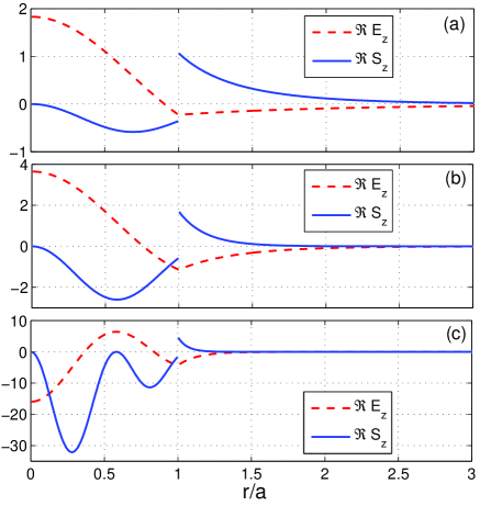
Figure 7: (Color online) The longitudinal electric field and Poynting vector for the first three TM mode on an anisotropic waveguide of radius $a$ with $\varepsilon_{t}=-3+0.05i$ and $\varepsilon_{z}=2$ at $k_{0}a=1.6$ with (a) $\beta a=1.7112+0.0067i$, (b) $\beta a=2.7250-0.0397i$, (c) $\beta a=7.5756-0.0676i$. The imaginary parts $\Im E_{z}$ and $\Im S_{z}$ are small and not plotted.

There is an interesting feature of the modes on the anisotropic waveguide. At a fixed $k_{0}$, for $a<a_{m}\equiv\sqrt{-\varepsilon_{t}/\varepsilon_{z}(1-\varepsilon_{t})}x_{0,m}/k_{0}$, the $m$-th band TM modes are backward waves. If the radius $a>a_{m}$, the waveguide supports two TM modes for the $m$-th band, one forward and one backward. At $a=a_{c}$, these two modes become degenerate and the total energy flow is zero. This can be seen in Fig. 2, 3, 6 where degenerate points are marked. Further increasing the radius, the waveguide will no longer support the $m$-th band. The critical radius $a_{c}$ is located such that $\langle P_{z}\rangle=0$, $d(k_{0}a)/d(\kappa_{0}a)=0$ or $dn_{\rm eff}/da=\infty$. These degenerate modes can be used to slow down and even trap light. This will be discussed in the next section.

II.3 Hybrid modes

The modes with both $E_{z}\neq 0$ and $H_{z}\neq 0$ are called hybrid modes. Their dispersions are contained in the solutions of Eq. (14) with $n\neq 0$. We recast the equation in the following form

$$\varepsilon_{z}f_{n}(Ka)=g_{n}(\xi)-{n^{2}(\xi^{-2}-y^{-2})(\xi^{-2}-\varepsilon_{t}y^{-2})\over g_{n}(\xi)+h_{n}(y)}.$$ (31)

Here we use the notation $\xi=\kappa_{0}a$ and $y=\kappa a$. Note that $Ka=y/\eta$ with $\eta=\sqrt{-\varepsilon_{t}/\varepsilon_{z}}$.

II.3.1 Band structure of hybrid modes

At a fixed wavelength $\lambda$ or wave number $k_{0}$, $\varepsilon_{t}$, $\varepsilon_{z}$ are constant. Since $Ka=y/\eta$, if we use $\xi=\kappa_{0}a$ as a free parameter, the eigen equation gives a single value of $Ka$ or $y$ for each $\xi$. Since $y=\sqrt{\xi^{2}+(1-\varepsilon_{t})(k_{0}a)^{2}}$, so the eigen equation actually gives the reduced radius $k_{0}a$ for each $\xi=\kappa_{0}a$.

In the limit of long wavelength or small waveguide radius, $k_{0}a\to 0$, Eq. (31) is reduced to

$$\varepsilon_{z}f_{n}(\xi/\eta)=g_{n}(\xi).$$ (32)

This will give a discrete set of solutions $\kappa_{0}a=\xi_{n,m}$ for each $n$. For $\eta$ and $\varepsilon_{z}$ not very small, the values $\xi_{n,m}$ can be obtained approximately by making use of the asymptotic behavior $g_{n}(x)\sim x^{-1}$ for $x\to\infty$ and the Padé approximant of $f_{n}(x)$, which will be discussed in the Appendix. The anisotropic waveguide supports infinite number of hybrid modes, no matter how thin the waveguide is.

Close to the light line, $\xi\to 0$, the eigen equation can be simplified. We consider the hybrid modes with different $n$ separately.

For $n=1$, one has $g_{1}(x)\simeq x^{-2}-\ln(x/2)-\gamma$ for $x\to 0$, thus Eq. (31) becomes

$$\varepsilon_{z}f_{1}(Ka)\simeq-2\big{(}\ln{\xi\over 2}+\gamma\big{)}+h_{1}(y)+{1+\varepsilon_{t}\over y^{2}}.$$ (33)

with $\xi\ll y$. One has the solution $Ka\to x_{1,m}$ for $\xi\to 0$. Note that throughout this paper, we use $x_{n,m}$ to denote the $m$-th zero of $J_{n}(x)$. Also that $x_{n,0}=0$ for $n\geq 1$. Since $x_{1,0}=0$, special care should be taken for solutions $Ka\sim 0$. Making use of the asymptotic behaviors $h_{n}(x)\simeq nx^{-2}+1/[2(n+1)]$ and $f_{n}(x)\simeq nx^{-2}-1/[2(n+1)]$ for $x\to 0$ with $n\geq 1$, one gets

$$Ka\simeq{1\over\eta}\sqrt{1+\varepsilon_{t}\over\ln(\xi/2)+\gamma-(\varepsilon_{z}+1)/8}.$$ (34)

From this expression, one can see that only if $\varepsilon_{t}<-1$, there will be solution for $Ka\sim 0$ when $\xi\to 0$. The above expression gives the dispersion of the first band with $n=1$. The $m$-th band will start with $Ka=x_{1,m-1}$ and end with $Ka=\xi_{1,m}/\eta$. One has $\xi_{1,1}<\eta x_{1,1}$. However if $-1<\varepsilon_{t}<0$, there will be no solution for $Ka<x_{1,1}$. All the allowed modes will have finite $Ka$. For the $m$-th band, one has $x_{1,m}\leq Ka\leq\xi_{1,m}/\eta$ with $\xi_{1,1}>\eta x_{1,1}$. The first band starts with $Ka=x_{1,1}$. For any $x_{1,m}>0$, one has

$$Ka\simeq x_{1,m}-{\varepsilon_{t}x_{1,m}\over(\eta x_{1,m})^{2}[-2(\ln(\xi/2)+\gamma)+h_{1}(\eta x_{1,m})]+\varepsilon_{t}+1}.$$ (35)

The hybrid modes near the light line with $n=1$ are all forward waves.

For $n\geq 3$, one has the following asymptotic behavior of $g_{n}(x)$ for $x\to 0$,

$$g_{n}(x)\simeq{n\over x^{2}}+{1\over 2(n-1)}+ax^{2}.$$ (36)

with $a=-1/[8(n-2)(n-1)^{2}]$. The eigen equation (31) is reduced to

$$a^{2}{\xi}^{6}+c_{2}\xi^{4}+c_{1}\xi^{2}+c_{0}=0$$ (37)

with

$$c_{2} = a\Big{(}{1\over n-1}+h_{n}-\varepsilon_{z}f_{n}\Big{)},$$

$$c_{1} = 2na+{1\over 4(n-1)^{2}}+{h_{n}-\varepsilon_{z}f_{n}\over 2(n-1)}-\varepsilon_{z}f_{n}h_{n}-n^{2}{\frac{\varepsilon_{t}}{y^{4}}},$$

$$c_{0} = {n\over n-1}+n(h_{n}-\varepsilon_{z}f_{n})+{n^{2}(1+\varepsilon_{t})\over y^{2}}.$$ (38)

The eigen modes on the light line are given by the equation $c_{0}=0$. The exsitence of solution requires that $c_{0}\geq 0$. Only the positive root with small magnitude of the above cubic polynomial will give the dispersion for the modes near the light line. Since $\xi$ is small, the physical solution can be approximated as $\xi^{2}=-c_{0}/c_{1}-c_{2}c_{0}^{2}/c_{1}^{3}-a^{2}c_{0}^{3}/c_{1}^{4}$. Those modes all have $Ka>x_{n,m}$ for the $m$-th band.

For $n=2$, the asymptotic behavior of $g_{n}(x)$ is still given by Eq. (36), but with a non-constant coefficient $a=[\ln(x/2)+\gamma]/4$. The eigen equation near the light line is reduced further from Eq. (37) to

$$(\kappa_{0}a)^{2}\big{(}\ln{\kappa_{0}a\over 2}+\gamma\big{)}+c_{0}=0$$ (39)

with $c_{0}$ given in Eq. (38) with $n=2$.

For the allowed eigenmodes of the $m$-th hybrid band, one has the range $0\leq\kappa_{0}a<\xi_{n,m}$ with $\xi_{n,m}$ the solutions of Eq. (32). The solutions near both ends of the above range can be obtained analytically as we have done. For arbitrary $\xi$ within this range, the solution must be obtained numerically. However only when $\varepsilon_{t}<-1$, one can have eigenmodes with $0<Ka<x_{n,1}$. For the $m$-th band, one has $x_{n,m}<Ka\leq\xi_{n,m}/\eta$. Otherwise, the solution for the first band requires $x_{n,1}<Ka\leq\xi_{n,1}/\eta$ with $\xi_{n,1}>\eta x_{n,1}$. The band structure for hybrid modes on a waveguide with $\varepsilon_{t}=-3$ and $\varepsilon_{z}=2$ is shown in Fig. 8. The effective index of the waveguide $n_{\rm eff}\equiv\beta/k_{0}$ is also evaluated and plotted in Fig. 9.

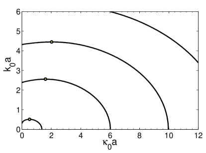
Figure 8: Band structure of the guided hybrid modes with $n=1$ on an anisotropic waveguide with $\varepsilon_{t}=-3$ and $\varepsilon_{z}=2$. Open circles denote the degeneracy of forward-wave and backward-wave modes.

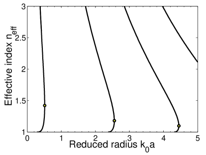
Figure 9: Effective index $n_{\rm eff}$ as a function of the reduced radius $k_{0}a$ for the first three bands of hybrid modes with $n=1$ on an anisotropic waveguide with $\varepsilon_{t}=-3$ and $\varepsilon_{z}=2$. Open circles denote the degeneracy of forward-wave and backward-wave modes.

II.3.2 Energy flow of hybrid modes

The energy flow can also be evaluated for hybrid modes. The expression for $S_{z}$ is much more complex than that of the TM modes. However the final expression for $P_{z}$ is much simpler than expected, once the integrals are all carried out. One has

$$P_{z}^{\rm in} = {\beta\over 4k_{0}}\Bigg{\{}-{\varepsilon_{z}^{2}\over\varepsilon_{t}Ka}(g_{n}+h_{n})f^{\prime}_{n}-{1\over\kappa a}(g_{n}-\varepsilon_{z}f_{n})h^{\prime}_{n}$$

$$+{2n^{2}\over(\kappa a)^{4}}\Big{[}{1+\varepsilon_{t}\over(\kappa_{0}a)^{2}}-{2\varepsilon_{t}\over(\kappa a)^{2}}\Big{]}\Bigg{\}},$$

$$P^{\rm out}_{z} = {\beta\over 4k_{0}}\Bigg{\{}-{1\over\kappa_{0}a}(2g_{n}+h_{n}-\varepsilon_{z}f_{n})g^{\prime}_{n}$$ (40)

$$-{2n^{2}\over(\kappa_{0}a)^{4}}\Big{[}{2\over(\kappa_{0}a)^{2}}-{1+\varepsilon_{t}\over(\kappa a)^{2}}\Big{]}\Bigg{\}}.$$

Here $f^{\prime}_{n}$, $g^{\prime}_{n}$, and $h^{\prime}_{n}$ are the derivatives of $f_{n}$, $g_{n}$, and $h_{n}$, respectively. In this derivation, we assume $\varepsilon_{t}$ and $\varepsilon_{z}$ are real, thus the arguments of the Bessel functions are all real. We set $A=\sqrt{g_{n}+h_{n}}/(k_{0}aJ_{n})$. Use has also been made of the following integrals which can not be found in any mathematics manual

$$\int_{0}^{x}\big{(}J^{\prime 2}_{n}(x)+{n^{2}\over x^{2}}J_{n}^{2}(x)\big{)}xdx = -{x^{3}\over 2}J^{2}_{n}(x)f^{\prime}_{n}(x),$$

$$\int_{0}^{x}\big{(}I^{\prime 2}_{n}(x)+{n^{2}\over x^{2}}I^{2}_{n}(x)\big{)}xdx = -{x^{3}\over 2}I^{2}_{n}(x)h^{\prime}_{n}(x),$$

$$\int_{x}^{\infty}\big{(}K^{\prime 2}_{n}(x)+{n^{2}\over x^{2}}K^{2}_{n}(x)\big{)}xdx = -{x^{3}\over 2}K^{2}_{n}(x)g^{\prime}_{n}(x).$$ (41)

Explicitly, one has

$$f^{\prime}_{n}(x) = -xf^{2}_{n}(x)-{2\over x}f_{n}(x)+{n^{2}\over x^{3}}-{1\over x},$$

$$h^{\prime}_{n}(x) = -xh^{2}_{n}(x)-{2\over x}h_{n}(x)+{n^{2}\over x^{3}}+{1\over x},$$

$$g^{\prime}_{n}(x) = xg^{2}_{n}(x)-{2\over x}g_{n}(x)-{n^{2}\over x^{3}}-{1\over x}.$$ (42)

We point out that the above expressions for $P_{z}$ can be readily modified for dielectric or metallic cylindrical waveguide with the exchange of $f_{n}(ix)=-h_{n}(x)$ and $ixf^{\prime}_{n}(ix)=-xh^{\prime}_{n}(x)$.

The normalized energy flow on a waveguide with $\varepsilon_{t}=-3$ and $\varepsilon_{z}=2$ for the hybrid modes with $n=1,2,3$ is plotted in Fig. 10.

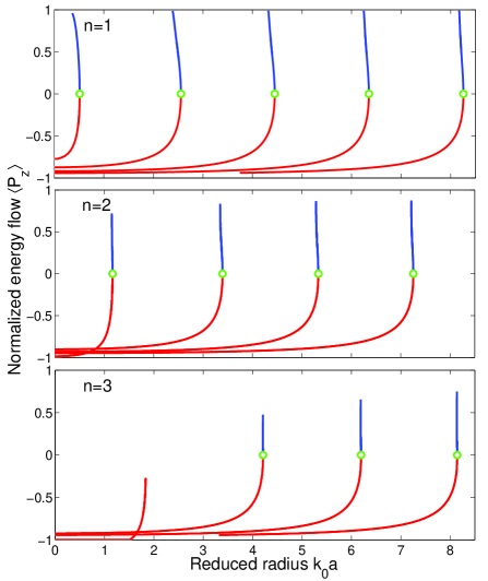
Figure 10: (Color online) Normalized energy flow $\langle P_{z}\rangle$ for the first few bands of the hybrid modes with $n=1,2,3$ on an anisotropic waveguide with $\varepsilon_{t}=-3$ and $\varepsilon_{z}=2$. Open circles denote the degeneracy points where $\langle P_{z}\rangle=0$.

II.3.3 Backward-wave and forward-wave hybrid modes

The hybrid modes have similar features as the TM modes that both forward waves and backward waves can co-exist within the same band. For $k_{0}a\to 0$, $\kappa\simeq\kappa_{0}$, the hybrid modes have $d(k_{0}a)/d(\kappa_{0}a)<0$ and are all backward waves. Only the modes near the light line can be forward waves. Making use of the expressions for $P_{z}$ in Eq. (40), one can prove that $d(k_{0}a)/d(\kappa_{0}a)\geq 0$ leads $P_{z}\geq 0$ and vice versa. The degeneracy of forward- and backward-wave modes is located at $d(k_{0}a)/d(\kappa_{0}a)=0$ or $\langle P_{z}\rangle=0$.

For the hybrid modes with $n=1,2$, the modes near the light line are forward waves since $d(k_{0}a)/d(\kappa_{0}a)>0$. However as can be seen in Fig. 10, the whole first band of the hybrid modes with $n=3$ are backward waves. Hybrid modes with higher $n$ will have more bands to be all backward waves. If one further increases the angular index $n$ of the hybrid modes, more hybrid mode bands will be all backward waves.

III Slow and trapped light

Recently Tsakmakidis et al Tsakmakidis proposed to trap light in a tapered waveguide with double negative index. The indefinite index waveguide we have studied so far in this paper can also be used to slow down and trap light. These waveguides can thus be used as optical buffers XiaF . The reason is that unlike the ordinary optical fiber, these waveguides support both forward and backward waves.

For the anisotropic waveguide we have considered, $\varepsilon_{t}<0$, one has $P^{\rm in}_{z}<0$ and $P^{\rm out}_{z}>0$ if one sets $\beta>0$. If $P_{z}=P^{\rm in}_{z}+P^{\rm out}_{z}<0$, the mode is a backward mode since the total energy flow is opposite to the phase velocity. Otherwise, the mode is a forward mode. At the critical radius $a_{c}$, the backward and forward modes become degenerate, the energy flow inside the waveguide cancels out that in the air. One can prove that at the critical radius $a_{c}$ where $P_{z}=0$, the group velocity is indeed zero. One does not need to know the material dispersion to locate the zero group velocity point. This is due to the fact that for these waveguides, the dispersion due to geometric confinement dominates the material dispersion at and around the critical radius.

The unique properties of the modes on anisotropic waveguide can be used to slow down and even trap light. Even though the waveguide supports infinite number of both TM and hybrid modes at any fixed radius and frequency, with appropriate laser coupling, the excitation of the hybrid modes in the waveguide can be suppressed or even eliminated. Among the TM modes, the first TM mode will be more favorably excited. Furthermore, due to the material dissipation, the first TM mode will propagate the longest distance. The rest of the TM modes will all decay out at about half the decay length of the first TM mode. It is the first TM band which can be used for slow light application. Unlike the double negative waveguide Tsakmakidis , the anisotropic waveguide will slow down and trap light if one increases the radius to the critical radius. A sketch of a slow light waveguide is shown in Fig. 11.

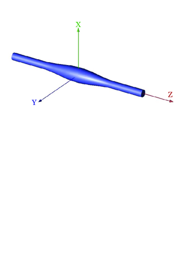
Figure 11: (Color online) A sketch of the slow light waveguide.

IV Realization of extremely anisotropic nanowires

These extremely anisotropic media can be realized in metamaterials. According to the effective medium theory Sihvola ; Lu07 , one has for multilayered structure of dielectric $\varepsilon_{a}$ and metal $\varepsilon_{m}$, the effective permittivities are

$$\varepsilon_{t} = f\varepsilon_{m}+(1-f)\varepsilon_{a},$$

$$\varepsilon_{z} = {\varepsilon_{a}\varepsilon_{m}\over f\varepsilon_{a}+(1-f)\varepsilon_{m}}.$$ (43)

Here $f$ is the filling ratio of the metal. For $f>f_{\rm min}\equiv\varepsilon_{a}/(\varepsilon_{a}-\Re\varepsilon_{m})$, one has $\Re\varepsilon_{t}<0$. A realization of the anisotropic nanowire is shown in Fig. 12.

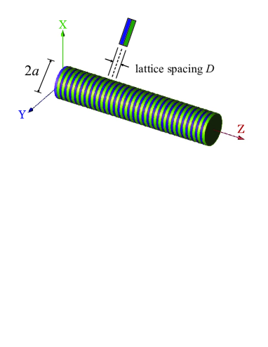
Figure 12: (Color online) A sketch of the realization of an anisotropic nanowire made of alternative disks of metal and dielectric.

We first consider a metamaterial waveguide at a fixed wavelength. For silver at $\lambda=488$ nm, one has $\varepsilon_{m}=-9.121+0.304i$ Palik . A nanowire made of alernative disks of silver and glass ($\varepsilon_{a}=2.25$) of equal thickness will have $\varepsilon_{t}=-3.436+0.152i$ and $\varepsilon_{z}=5.971+0.065i$ by using the effective medium theory. Here the disk thickness is 10 nm for both materials. For example if one sets $a=60$ nm, one has $k_{0}a=0.7725$. The first three TM modes will have $\beta a=2.2525-0.0747i,4.9318-0.1419i,7.4031-0.2088i$. Thus one has $\lambda_{\beta}\sim 167$ nm and phase refractive index $n_{\rm eff}=2.92$ for the first TM mode. The decay length is 803, 423, and 287 nm, respectively. After traveling about 420 nm along the nanowire, only the first one will survive.

Finite-difference time-domain (FDTD) simulations Taflove were performed to obtain the effective index $n_{\rm eff}$ of the metamaterial nanowire. The procedure is the following. We illuminate the free-standing nanowire of finite length with a Gaussian beam, then get $E_{z}$ after the termination of the simulation. The length of the waveguide is set to be larger than the decay length of the first TM mode. We get the phase from $E_{z}$, then determine $\beta$. Though the waveguide supports infinite number of modes including TM and hybrid modes, our method is legitimate due to the following two reasons. First that the excitation of hybrid modes is small due to the profile of the incident Gaussion beam. So mainly the TM modes are excited. Second that due to the dissipation in the metal, after certain distance, only the first TM mode will survive. Thus the phase propagation is mainly due to the first TM mode. The amplitide and phase propagation of $E_{z}$ along the above metamaterial nanowire is shown in Fig. 13.

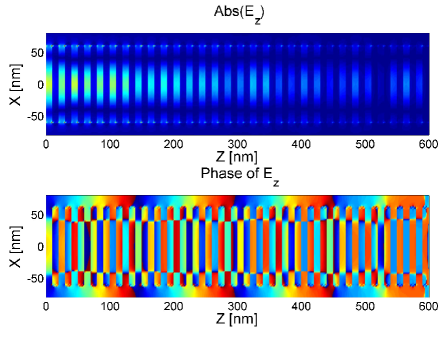
Figure 13: (Color online) FDTD simulation of the amplitude and phase propapation of the longitudinal electric field $E_{z}$ along the nanowire with radius $a=60$ nm at $\lambda=488$ nm. The metamaterial nanowire consists of alternative disks of silver and glass disks of thickness 10 nm.

The relation between the effective index $n_{\rm eff}$ and the nanowire radius $a$ is shown in Fig. 14. Very good agreement between FDTD simulations and analytical results has been obtained. However for small radius, there is noticeable discrepancy. This is expected since when the radius is comparable with the lattice spacing of the multilayered metamaterial, the effective medium theory will fail. We have also performed FDTD simulations for the nanowire with smaller lattice spacing. Better agreement is indeed obtained.

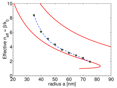
Figure 14: (Color online) The effective index $n_{\rm eff}$ of the first TM band on a nanowire with different radius at $\lambda=488$ nm. The nanowire is made of alternative disks of silver and (see Fig. 12). The disk thickness is 10 nm. Filled circle (green) is obtained from FDTD simulations. The dashed line (blue) is the fitting of simulation data. The solid line (red) is calculated from band equation with effective index $\varepsilon_{t}=-3.436+0.152i$ and $\varepsilon_{z}=5.971+0.065i$.

We also consider the band structure for different frequencies. The permittivity given by Eq. (24) can be realized through the multilayered heterostructure with Drude metal with $\varepsilon_{m}=1-k_{p}^{2}/k_{0}$ and dielectric $\varepsilon_{a}$. The nanowire is made of alternative disks of a Drude metal and a dielectric. The band structure and the effective index $n_{\rm eff}$ of the TM modes are shown in Fig. 4 and Fig. 5, respectively. One noticeable feature of these bands is the flatness of each band, which indicates small group velocity. We have erformed the FDTD simulation for different frequencies for nanowire with a fixed radius. The results are shown in Fig. 15. Again good agreement between FDTD simulations and analytical results is achieved.

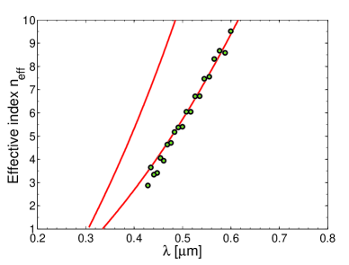
Figure 15: (Color online) The effective index $n_{\rm eff}$ for the TM modes on a nanowire with radius $a=40$ nm. The nanowire is a stack of equally thick alternative disks made of a Drude metal $\varepsilon_{m}=1-k_{p}^{2}/k_{0}(k_{0}+i\Gamma)$ and glass. Here $k_{p}a=1.64$ and $\Gamma a=0.0155$. The analytical curves (solid) are calculated by using real $\varepsilon_{m}$.

V conclusions

Indefinite index materials can be used to achieve negative refraction Hoffman and hyperlensing LiuZ ; Smolyaninov . They can also be used as superlens Lu07 . In this paper, we consider the wave propagation along a cylindrical waveguide with anisotropic optical constant. We have derived the eigenmodes equation and obtained the solutions for all the propagation modes. The field profiles and the energy flow on the waveguide are also analyzed. Closed-form expressions for the energy flow for all the modes are derived. For extremely anisotropic cylinder where the transverse component of the permittivity is negative and the longitudinal is positive ($\varepsilon_{t}<0$, $\varepsilon_{z}>0$), the waveguide supports TM and hybrid modes but not the TE modes. Among the supported TM modes, at most only one mode can be forward wave. The rest of them are backward waves.

The case that $\varepsilon_{t}>0$ and $\varepsilon_{z}<0$ can be discussed similarly. Anisotropic waveguides of cross section other than circle were also considered. The results will be published elsewhere.

Possible realization of these extremely anisotropic nanowires are proposed. Extensive FDTD simulations have been performed and confirmed our analytical results.

Two unique properties have been revealed for the modes on nanowire waveguides made of indefinite index metamaterials. The first is that the backward-wave modes can have very large effective index. These nanowires can be used as phase shifters and filters in optics and telecommunication. The second is that the waveguide supports modes of zero group velocity. This is due to the fact that the waveguide can support both forward and backward waves at a fixed radius. If the waveguide is tapered, at certain critical radius, the two modes will be degenerate and carry zero net energy flow. At other radii, these waveguides support modes with small group velocity. These waveguides can also be used as ultra-compact optical buffer XiaF in integrated optical circuits.

Appendix A Padé approximant of $f_{n}(x)$

Consider the function $f_{n}(x)=J^{\prime}_{n}(x)/[xJ_{n}(x)]$. Let $x_{n,m}$ be the $m$-th zero of the Bessel function $J_{n}(x)$. We also denote $x^{\prime}_{n,m}$ as the zeros of $J^{\prime}_{n}(x)$. In order to get the eigen modes on the anisotropic waveguide easily, we may need the inverse function $f^{-1}_{n}(x)$ in the interval $[x_{n,m},x^{\prime}_{n,m}]$. We consider the Padé approximant to the function $f_{n}(x)$,

$$f_{n}(x)\simeq{(x-x^{\prime}_{n,m})(x-x_{n,m}-b)\over c(x-x_{n,m})(x-x_{n,m}-a)}.$$ (44)

Instead of fixing the three unknowns through the coefficients of the Taylor expansion of $f_{n}(x)$, here we determine them by the exact values of $f_{n}(x)$ at some points. Since there are three unknowns, we only need the value of $f_{n}(x)$ at three points. For simplicity, we evaluate $f_{n}(x)$ at three evenly spaced points

$$f_{n,j}\equiv f_{n}(x_{n,m}+j\Delta/4)$$ (45)

for $j=1,2,3$. Here $\Delta=x^{\prime}_{n,m}-x_{n,m}$. One thus has $f_{n,j}=(4-j)(j\Delta-4b)/[jc(j\Delta-4a)$. We further define

$$\sigma_{1}=3f_{n,2}/f_{n,1},\quad\sigma_{2}=3f_{n,3}/f_{n,2}.$$ (46)

After some manipulations of the algebra, one obtains

$$a = {\Delta\over 4}\Big{(}2+{\sigma_{2}-\sigma_{1}^{-1}\over\sigma_{2}+\sigma_{1}^{-1}-2}\Big{)},$$

$$b = {\Delta\over 4}\Big{(}2-{\sigma_{1}-\sigma_{2}^{-1}\over\sigma_{1}+\sigma_{2}^{-1}-2}\Big{)},$$

$$c = -{1\over f_{2}}{\Delta-2b\over\Delta-2a}.$$ (47)

The inverse of the function $f_{n}(x)$ can be obtained as one of the roots of a quadratic equation. As it turns out, the expression obtained in this way gives very good approximation to $f^{-1}_{n}(x)$.

Once the inverse function is obtained, one has $Ka=f^{-1}_{0}(y)$ with $y=g_{0}(\kappa_{0}a)/\varepsilon_{z}$ for the TM modes. Together with the asymptotic expressions of $g_{n}(x)$ and $h_{n}(x)$, Eq. (44) can also be used to obtain approximate solutions of the hybrid modes.

References

- (1) V. Veselago, Soviet Physics USPEKHI 10, 509 (1968).
- (2) R. A. Shelby, D. R. Smith, and S. Schultz, Science 292, 77 (2001).
- (3) J. B. Pendry, Phys. Rev. Lett. 85, 3966 (2000).
- (4) W. T. Lu and S. Sridhar, Opt. Express 13, 10673 (2005).
- (5) W. T. Lu and S. Sridhar, Microwave Opt. Tech. Lett. 39, 282 (2003).
- (6) N. Fang et al., Science 308, 534 (2005).
- (7) P. Vodo, P. V. Parimi, W. T. Lu, and S. Sridhar, Appl. Phys. Lett. 86, 201108 (2005).
- (8) P. Vodo, W. T. Lu, Y. Huang, and S. Sridhar, Appl. Phys. Lett. 89, 084104 (2006).
- (9) C. G. Parazzoli et al., Phys. Rev. Lett. 90, 107401 (2003).
- (10) P. V. Parimi et al., Phys. Rev. Lett. 92, 127401 (2004).
- (11) P. V. Parimi, W. T. Lu, P. Vodo, and S. Sridhar, Nature (London) 426, 404 (2003).
- (12) E. Cubukcu et al., Nature (London) 423, 604 (2003).
- (13) Z. Lu et al., Phys. Rev. Lett. 95, 153901 (2005).
- (14) A. Berrier et al., Phys. Rev. Lett. 93, 073902 (2004).
- (15) G. Dolling, C. Enkrich, M. Wegener, C. M. Soukoulis, and S. Linden, Science 312, 892 (2006).
- (16) C. M. Soukoulis, S. Linden, and M. Wegener, Science 315, 47 (2007).
- (17) D. R. Smith, J. B. Pendry, and M. C. Wiltshire, Science, 305, 788 (2004).
- (18) M. Notomi, Phys. Rev. B 62, 10696 (2000).
- (19) B. Gralak, S. Enoch, and G. Tayeb, J. Opt. Soc. Am. A 17, 1012 (2000).
- (20) C. Luo et al., Phys. Rev. B 65, 201104 (2002).
- (21) V. M. Shalaev, Nat. Photonics 1, 41 (2007).
- (22) J. D. Joannopoulos, R. D. Meade, and J. N. Winn, Photonic Crystals: Molding the Flow of Light, Princeton Univ. Press (1995).
- (23) D. Schurig, J. J. Mock, B. J. Justice, S. A. Cummer, J. B. Pendry, A. F. Starr, D. R. Smith, Science 314, 977 (2006).
- (24) D. R. Smith and D. Schurig, Phys. Rev. Lett. 90, 077405 (2003); D. R. Smith, P. Kolinko, and D. Schurig, J. Opt. Soc. Am. B 21, 1032 (2004).
- (25) A. J. Hoffman et al., Nat. Mat. 6, 946 (2007).
- (26) W. T. Lu and S. Sridhar, preprint, arXiv: cond-mat.0710.4933 (2007).
- (27) Z. Liu et al., Science 315, 1686 (2007).
- (28) I. I. Smolyaninov, Y.-J. Hung, and C. C. Davis, Science 315, 1699 (2007).
- (29) J. Takahara et al., Opt. Lett. 22, 475 (1997).
- (30) K. L. Tsakmakidis, A. Klaedtke, D. A. Aryal, C. Jamois, and O. Hess, Appl. Phys. Lett. 89, 201103 (2006).
- (31) K. L. Tsakmakidis, A. D. Boardman, and O. Hess, Nature 450, 397 (2007).
- (32) F. Xia, L. Sekaric, and Y. Vlasov, Nat. Photonics 1, 65 (2007).
- (33) A. Sihvola, Electromagnetic mixing formulas and applications, The Institute Of Electrical Engineers, London (1999).
- (34) E. D. Palik, Handbook of Optical Constants of Solids, Academic Press (1981).
- (35) A. Taflove and S. C. Hagness, Computational Electrodynamics: The Finite-Difference Time-Domain Method, 3rd ed., Artech House Publishers, Norwood, MA (2005).