Probabilistic Embedding Of Discrete Sets As Continuous Metric Spaces

Abstract

Any symmetric affinity function $w:V\times V\to\mathbb{R}_{+}$ defined on a discrete set $V$ induces Euclidean space structure on $V$. In particular, an undirected graph specified by an affinity (or adjacency ) matrix can be considered as a metric topological space. We have calculated the visual representations of the probabilistic locus for a chain, a polyhedron, and a finite 2-dimensional lattice.

1 Introduction

Flatness is the essential property of Euclidean space. In particular, there is no distinguished point that serves as an origin, because it can be translated anywhere. This affine-geometric property of Euclidean space is generalized by the affine group of all invertible affine transformations from the space into itself consisting of a linear transformation described by a matrix $\mathcal{A}$ followed by a translation,

$$\bf{y}\,=\,\mathcal{A}\bf{x}+\bf{a}.$$

It is known that the affine geometry keeps the concepts of straight lines and parallel lines but not those of distance between points or value of angles, [1].

From a probabilistic point of view, the fact that there is no canonical choice of the origin can be interpreted as if it can be at any point in the space with a uniform probability. The interesting question arises when the probability $\pi_{x}>0$ to find the origin at the particular point $x\in V$ of some discrete set $V$ of $N$ points is not uniform,

$$\sum_{x\in V}\pi_{x}\,=\,1,$$ (1)

– What does such a space look like?

One way to describe the disparity between points in the set $V$ is by introducing an affinity function $w:V\times V\to\mathbb{R}_{+}\cup\{0\}$ encoding their pairwise relations or neighborhoods - two points $x\in V$ and $y\in V$ are neighbors, $x\sim y$, iff $w_{xy}>0$, but $w_{xy}=0$ otherwise. Then, the probability distribution $\pi$ is given by

$$\pi_{x}\,=\,\frac{\,\,\sum_{y\in V}w_{xy}\,\,}{\,\,\sum_{y,z\in V}w_{yz}\,\,}.$$ (2)

The affinity function $w_{xy}\geq 0$ defines an undirected weighted graph $G(V,E)$, in which $V$ is the set of nodes and $E\subseteq V\times V$ is the set of edges describing the relation between pairs of nodes.

The aim of this paper is to investigate the properties of the probabilistic locus satisfying (1) (a graph) specified by the arbitrary symmetric, non-degenerated matrix $w_{xy}\geq 0$ and to show that it can be regarded as the projective space $P\mathbb{R}^{(N-1)}$ of homogeneous coordinates obtained by projection from the origin $\pi$. Given a random walk defined on the graph $G(V,E)$, the projective geometry can be reduced to the metric geometry, which is realized by the introduction of a Euclidean scalar product, a distance, and a norm which can be directly related to the first-access times of nodes by random walkers.

The paper is organized as follows. In (Sec. 2), we introduce the probabilistic analog of affinity transformations that can be interpreted as random walks defined on the set $V$ with the structure determined by the matrix $w_{xy}\geq 0$. In (Sec. 3), we consider the probabilistic projective geometry for the space projected from the distinguished probability distribution $\pi$ induced by a simple stochastic process - a random walk - instead a distinguished point as in the usual projective geometry. In (Sec. 4), we perform a reduction from the probabilistic projective geometry to the probabilistic metric geometry by introducing the Euclidean space structure associated to the diffusion process defined on $V$ with respect to $w_{xy}\geq 0$. Then, in (Sec. 5), we demonstrate that the Euclidean characteristics can be interpreted in terms of the first-access properties of nodes by random walkers. Using the metric structure introduced in Sec. 4, we introduce a probabilistic topological space in Sec. 6. We conclude in Sec. 7 and give three visual representations of the probabilistic locus of a chain, a polyhedron, and a finite 2-dimensional lattice.

2 Probabilistic analog of affinity transformations

In a geometric setting, affine transformations [2] are precisely the functions that map straight lines to straight lines, i.e. preserves all linear combination in which the sum of the coefficients is 1. Their probabilistic analog in the class of stochastic matrices, $\sum_{y\in V}T_{xy}=1$, is given by the transition probability operators,

$$T_{xy}\,=\,\left(1-\beta_{x}\right)\delta_{xy}+\frac{\,\,\beta_{x}\,w_{xy}\,\,}{\,\,\sum_{y\in V}w_{xy}\,\,}$$ (3)

where $\beta_{x}\in\left[0,1\right]$ and $w_{xy}\geq 0$ is the symmetric affinity matrix describing the set of paths available from $x\in V$.

If points of the discrete set $V$ are interpreted as nodes of an undirected graph, then the transition operator (3) describes a ”lazy” random walk on $G(V,E)$ specified by the ”laziness” parameters $\beta_{x}$, such that a random walker stays in $x\in V$ with probability $1-\beta_{x}$, but moves to another node randomly chosen among the nearest neighbors with probability $\beta_{x}/\sum_{y}w_{yx}$. In particular, if $\beta_{x}=1$ uniformly for all $x\in V$, the operator (3) describes the usual random walks extensively studied in the classical surveys [3],[4].

Random walks provide us with an effective tool for the detailed structural analysis of connected undirected graphs exposing their symmetries. In [5], we have shown that the transition operator (3) gives the representation of the group of linear automorphisms of the undirected graph $G(V,E)$, in the class of stochastic matrices.

Discrete translational symmetry is obviously broken if the graph $G$ is either finite, or irregular. If the graph is finite but regular, then the transition probability operator (3) defines a symmetric Markov chain, in which the probability of moving to $y\in V$ given that a walker is at the node $x\in V$ is the same as the probability of moving backward. Finally, for a non-regular graph $G$ this property is replaced by time–reversibility that can be conveniently formulated in terms of the stationary random walks,

$$\pi_{x}T_{xy}\,=\,\pi_{y}T_{yx},$$ (4)

for every pair $x,y\in V$. It is well known (see [3]) that the stationary distribution of random walks $\pi$ defined on the undirected graph $G$ is given by (2) and is the left eigenvector of the transition operator (3) belonging to its primary Perron eigenvalue $\mu=1$. Since for any choice of $\beta_{x}\in[0,1]$ the matrix $T_{xy}\geq 0$ is a real positive stochastic matrix, it follows from the Perron-Frobenius theorem (see [8]) that its maximal eigenvalue $\mu=1$ is simple if the graph $G$ is connected. Any other distribution $\sigma$ defined on $V$ such that $\sigma_{x}\geq 0$ for any $x\in V$ and $\sum_{x\in V}\sigma_{x}=1$, asymptotically tends to the stationary distribution $\pi$ under the iterative actions of the transition operator (3),

$$\pi\,=\,\lim_{n\to\infty}\,\sigma\,T^{\,n}.$$ (5)

The self-adjoint operator associated to $T$ is given by

$$\widehat{T}\,=\,\frac{1}{2}\left(\pi^{1/2}T\pi^{-1/2}+\pi^{-1/2}T^{\top}\pi^{1/2}\right),$$ (6)

where $T^{\top}$ is the adjoint operator, and $\pi$ is defined as the diagonal matrix $\mathrm{diag}\left(\pi_{1},\ldots,\pi_{N}\right)$. While interesting in the spectral calculations of random walks characteristics, the symmetric matrix (6) is more convenient since its eigenvalues are real and bounded in the interval $\mu\in[-1,1]$ and the eigenvectors define an orthonormal basis.

3 Probabilistic projective geometry

An affine coordinate system on $V$ is prescribed by an affinely independent set of points for which the displacement vectors $\mathbf{e}_{y}={y}-{x}$, $y\in V$, $x\neq y$, form a basis of $V$ with respect to the point $x\in V$. A displacement vector $\mathbf{v}=\sum_{y\in V}v_{y}\mathbf{e}_{y}$ is identified with the coordinate $(N-1)$-tuple $\left(v_{1},\ldots,\{\,\,\}_{x},\ldots,v_{N}\right)$, in which the $x-$th component is missing. We can associate all points $V$ with their relative displacement vectors.

This is the distinguished probability distribution $\pi$ induced by a simple stochastic process - a random walk - is important for the defining an elementary coordinate system in the probabilistic projective space. Given a symmetric matrix $w_{xy}\geq 0$ and a vector $\beta_{x}\in[0,1]$, we can define the transition probability by the kernel (3) on $V$ and its self-adjoint counterpart (6). The complete set of real eigenvectors $\Psi=\{\psi_{1},\psi_{2},\ldots\psi_{N}\}$ of the symmetric matrix (6),

$$\left|\psi_{i}\right\rangle\widehat{T}\,=\,\mu_{i}\left|\psi_{i}\right\rangle,$$

ordered in accordance to their eigenvalues, $\mu_{1}=1>\mu_{2}\geq\ldots\mu_{N}\geq-1$, forms an orthonormal basis in $\mathbb{R}^{N}$,

$$\left\langle\psi_{x}|\psi_{y}\right\rangle\,=\,\delta_{xy},$$ (7)

associated to linear automorphisms of the affinity matrix $w_{xy}$, [5]. In (7), we have used Dirac’s bra-ket notations especially convenient for working with inner products and rank-one operators in Hilbert space.

Given the random walk defined by the operator (3), then the squared components of the eigenvectors $\Psi$ have very clear probabilistic interpretations. The first eigenvector $\psi_{1}$ belonging to the largest eigenvalue $\mu_{1}=1$ satisfies $\psi_{1,x}^{2}=\pi_{x}$ and describes the probability to find a random walker in $x\in V$. The norm in the orthogonal complement of $\psi_{1}$, $\sum_{i=2}^{N}\psi_{i,x}^{2}\,=\,1-\pi_{x}$, is nothing else but the probability that a random walker is not in $x$.

Looking back it is easy to see that the transition operator (6) defines a projective transformation on the set $V$ such that all vectors in $\mathbb{R}^{N}(V)$ collinear to the stationary distribution $\pi>0$ (2) are projected onto a common image point.

Geometric objects, such as points, lines, or planes, can be given a representation as elements in projective spaces based on homogeneous coordinates, [9]. Any vector of the Euclidean space $\mathbb{R}^{N}$ can be expanded into $\mathbf{v}=\sum_{k=1}^{N}\left\langle\mathbf{v}|\psi_{k}\right\rangle\left\langle\psi_{k}\right|$, as well as into the basis vectors

$$\psi^{\prime}_{s}\equiv\left(1,\frac{\,\psi_{s,2}\,}{\,\psi_{s,1}\,},\ldots,\frac{\,\psi_{s,N}\,}{\,\psi_{s,1}\,}\right),\quad s\,=\,2,\ldots,N,$$ (8)

which span the projective space $P\mathbb{R}_{\pi}^{(N-1)}$,

$$\mathbf{v\pi}^{-1/2}\,=\,\sum_{k=2}^{N}\left\langle\mathbf{v}|\psi^{\prime}_{k}\right\rangle\left\langle\psi^{\prime}_{k}\right|,$$

since we have always $\psi_{1,x}\equiv\sqrt{\pi_{x}}>0$ for any $x\in V$. The set of all isolated vertices $p$ of the graph $G(V,E)$ for which $\pi_{p}=0$ play the role of the plane at infinity, away from which we can use the basis $\Psi^{\prime}$ as an ordinary Cartesian system. The transition to the homogeneous coordinates (8) transforms vectors of $\mathbb{R}^{N}$ into vectors on the $(N-1)$-dimensional hyper-surface $\left\{\psi_{1,x}=\sqrt{\,\pi_{x}\,}\right\}$, the orthogonal complement to the vector of stationary distribution $\pi$.

4 Reduction to metric geometry

The key observation is that in homogeneous coordinates the operator $\left.\widehat{T}^{k}\right|_{P\mathbb{R}_{\pi}^{(N-1)}}$ defined on the $(N-1)$-dimensional hyper-surface $\left\{\psi_{1,x}=\sqrt{\,\pi_{x}\,}\right\}$ determines a contractive discrete-time affine dynamical system. The origin is the only fixed point of the map $\left.\widehat{T}^{k}\right|_{P\mathbb{R}_{\pi}^{(N-1)}}$,

$$\lim_{n\to\infty}\widehat{T}^{\,n}\xi\,=\,\left(1,0,\ldots 0\right),$$ (9)

for any $\xi\in P\mathbb{R}_{\pi}^{(N-1)}$ and the solutions consist in the linear system of points $\widehat{T}^{\,n}\xi$ that hop in the phase space (see Fig. 1) along the curves formed by collections of points that map into themselves under the consecutive action of $\widehat{T}$.

Figure 1: Any vector $\xi\in P\mathbb{R}_{\pi}^{(N-1)}$ asymptotically approaches the origin $\pi$ under the consecutive actions of the operator $\widehat{T}$.

The problem of random walks (3,6) defined on finite undirected graphs can be related to a diffusion process which describes the dynamics of a large number of random walkers. The symmetric diffusion process correspondent to the self-adjoint transition operator $\widehat{T}$ describes the time evolution of the normalized expected number of random walkers, ${\bf n}(t)\,\pi^{-1/2}\in V\times\mathbb{N}$,

$$\dot{\bf n}\,=\,\widehat{L}{\bf n},\quad\widehat{L}\,\equiv\,1-\widehat{T}$$ (10)

where $\widehat{L}$ is the normalized Laplace operator. Eigenvalues of $\widehat{L}$ are simply related to that of $\widehat{T}$, $\lambda_{k}=1-\mu_{k}$, $k=1,\ldots,N$, and the eigenvectors of both operators are identical. The analysis of spectral properties of the operator (10) is widely used in the spectral graph theory, [6].

It is important to note that the normalized Laplace operator (10) defined on $P\mathbb{R}_{\pi}^{(N-1)}$ is invertible,

$$\begin{array}[]{lcl}\widehat{L}^{-1}&=&\left(1-\widehat{T}\right)^{-1}\\ &=&\sum_{n\geq 1}\widehat{T}^{n}.\end{array}$$ (11)

since $\left.\widehat{T}^{k}\right|_{P\mathbb{R}_{\pi}^{(N-1)}}$ is a contraction mapping for any $k\geq 1$. The unique inverse operator,

$$\widehat{L}^{-1}\,=\,\sum_{s=2}^{N}\frac{\,\,\left|\psi^{\prime}_{s}\right\rangle\left\langle\psi^{\prime}_{s}\right|\,\,}{\,\,1-\mu_{s}\,\,},$$ (12)

is the Green function (or the Fredholm kernel) describing long-range interactions between eigenmodes of the diffusion process induced by the graph structure. The convolution with the Green’s function gives solutions to inhomogeneous Laplace equations.

In order to apply metric geometry to the graph $G(V,E)$, one needs to introduce the distances between points (nodes of the graph) and the angles between lines or vectors that can be done by determining the inner product between any two vectors $\xi$ and $\zeta$ in $P\mathbb{R}_{\pi}^{(N-1)}$ as

$$\left(\xi,\zeta\right)_{(w,\beta)}\,=\,\left(\xi,\widehat{L}^{-1}\zeta\right).$$ (13)

The dot product (13) is a symmetric real valued scalar function that allows us to define the (squared) norm of a vector $\xi\in P\mathbb{R}_{\pi}^{(N-1)}$ with respect to $(w,\beta)$ by

$$\left\|\,\xi\,\right\|^{2}_{(w,\beta)}\,=\,\left(\xi,\widehat{L}^{-1}\xi\right).$$ (14)

The (non-obtuse) angle $\theta\in[0,180^{\mathrm{o}}]$ between two vectors is then given by

$$\theta\,=\,\arccos\left(\frac{\,\,\left(\xi,\zeta\right)_{(w,\beta)}\,\,}{\,\,\left\|\,\xi\,\right\|_{(w,\beta)}\left\|\,\zeta\,\right\|_{(w,\beta)}\,\,}\right).$$ (15)

The Euclidean distance between two vectors in $P\mathbb{R}_{\pi}^{(N-1)}$ with respect to $(w,\beta)$ is defined by

$$\begin{array}[]{lcl}\left\|\xi-\zeta\right\|^{2}_{(w,\beta)}&=&\left\|\,\xi\,\right\|^{2}_{(w,\beta)}+\left\|\,\zeta\,\right\|^{2}_{(w,\beta)}-2\left(\xi,\zeta\right)_{(w,\beta)}\\ &=&\mathbb{P}_{\xi}\left(\xi-\zeta\right)+\mathbb{P}_{\zeta}\left(\xi-\zeta\right)\end{array}$$ (16)

where $\mathbb{P}_{\xi}\left(\xi-\zeta\right)\equiv\left\|\,\xi\,\right\|^{2}_{(w,\beta)}-\left(\xi,\zeta\right)_{(w,\beta)}$ and $\mathbb{P}_{\zeta}\left(\xi-\zeta\right)\equiv\left\|\,\zeta\,\right\|^{2}_{(w,\beta)}-\left(\xi,\zeta\right)_{(w,\beta)}$ are the lengths of the projections of $(\xi-\zeta)$ onto the unit vectors in the directions of $\xi$ and $\zeta$ respectively. It is clear that $\mathbb{P}_{\zeta}\left(\xi-\zeta\right)=\mathbb{P}_{\xi}\left(\xi-\zeta\right)=0$ if $\xi=\zeta.$

It is worth mentioning that the spectral representations of the Euclidean structure (13-16) defined for the graph nodes can be easily derived by taking into account that $\left\langle x\right.\left|\psi^{\prime}_{s}\right\rangle=\psi^{\prime}_{s,x}$.

5 Euclidean structure and the first-access characteristic times of graph nodes

The structure of Euclidean space introduced in the previous section can be related to a length structure $V\times V\to\mathbb{R}_{+}$ defined on a class of all admissible paths $\mathcal{P}$ between pairs of nodes in $G$. It is clear that every path $P(x,y)\in\mathcal{P}$ is characterized by some probability to be followed by a random walker which in particular depends upon the weights $w_{pq}>0$ of all edges $p\sim q$ that join it. Therefore, the path length statistics is a natural candidate for the length structure on $G$.

The theory of random walks on graphs offers the concepts to quantify the mutual accessibility of nodes in a graph. The access time or hitting time $h_{xy}$ is the expected number of steps before node $y$ is visited, starting from node $x$, [3]. Since the first step takes a walker to a neighbor $v\sim x$ and then the walker has to reach $y$ from there, the hitting time should be additive,

$$h_{xy}\,=\,1+\frac{\,\,\sum_{x\sim v}h_{vy}\,\,}{\,\,\sum_{z\in V}w_{xz}\,\,}$$ (17)

if $x\neq y$ and $h_{xx}=0.$ In general $h_{xy}$ is not a symmetric matrix except if the graph has a vertex-transitive automorphism group, [3].

The sum

$$d(x,y)\,=\,h_{xy}+h_{yx}$$ (18)

is called the commute time: this is the expected number of steps in a random walk starting at $x$ before node $y$ is visited and then node $x$ is reached again, [3].

The expected number of steps to first arrival of a random walker at $x\in V$ starting from another node randomly chosen with respect to the probability $\pi$,

$$f_{x}\,=\,\sum_{y\in V}\pi_{y}h_{yx},$$ (19)

is called the first-passage time to $x$.

All three quantities are well-known in the theory of random walks on graphs and can be calculated in the standard way, [3]. The most important observation for us is that their spectral representations,

$$\begin{array}[]{lcl}h_{xy}&=&\sum_{s=2}^{N}\,\left(\psi^{\prime 2}_{s,x}-\psi^{\prime}_{s,x}\psi^{\prime}_{s,y}\right)^{2}/\left(1-\mu_{s}\right),\\ d(x,y)&=&\sum_{s=2}^{N}\,\left(\psi^{\prime}_{s,x}-\psi^{\prime}_{s,y}\right)^{2}/\left(1-\mu_{s}\right),\\ f_{x}&=&\sum_{s=2}^{N}\,\,\psi^{\prime 2}_{s,x}\,/\left(1-\mu_{s}\right),\end{array}$$ (20)

coincide with those of the Euclidean quantities, $\mathbb{P}_{x}(x-y)$, $\left\|x-y\right\|^{2}_{(w,\beta)}$, and $\left\|x\right\|^{2}_{(w,\beta)}$ respectively.

6 Probabilistic topological space

In the previous sections, we have shown that given a symmetric affinity function $w:V\times V\to\mathbb{R}_{+}$, we can always define an Euclidean metric on $V$ based on the first-access properties of the standard stochastic process, the random walks defined on the set $V$ with respect to the matrix $w_{xy}\geq 0$.

In particular, we can introduce this metric on any undirected graph $G(V,E)$ converting it in a metric space. The Euclidean distance interpreted as the commute time induces the metric topology on $G(V,E)$. Namely, we define the open metric ball of radius $r$ about any point $x\in V$ as the set

$$B_{r}(x)\,=\,\left\{y\in V:d(x,y)<r\right\}.$$ (21)

These open balls generate a topology on $V$, making it a topological space. A set $U$ in the metric space is open if and only if for every point $x\in U$ there exists and $\varepsilon>0$ such that $B_{\varepsilon}(r)\subset U$, [7]. Explicitly, a subset of $V$ is called open if it is a union of (finitely or infinitely many) open balls.

7 Conclusion and examples

Systems consisting of many individual units that are tied by one or more specific types of interdependency are found everywhere in the world. Networks are often very complex and difficult to analyze. Being of rather large scale to be seen from a single viewpoint, they can often be abstracted as graphs, the natural mathematical tool for facilitating the analysis.

1.		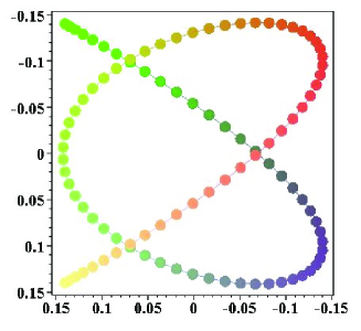2.
3.		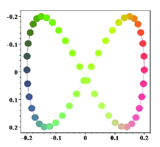4.

Figure 2: Probabilistic images of a chain ($N=100$) and a polyhedron ($N=50$).

Euclidean space has a decisive role in visual and propriomotor percepts, and in hearing thus determining our spatial perception. In addition, many of our feelings, of anger, fear and so on, have important links with parts of the body and hence indirectly with Euclidean space. In general, networks do not possess the structure of Euclidean space. Thus, a mental representation of any network emerges as a result of a long learning process jointly with the planning of movements in that and is always challenging to make the proper decisions on how to sustain the system and to cope with the new demand.

1.		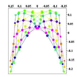2.

Figure 3: 1. Probabilistic image of a 2D-lattice ($N=10^{2}$). 2. The matrix plot of the probabilistic Euclidean distances (the commute times) between the nodes of the lattice $\mathcal{L}_{2}$.

In our paper, we have demonstrated that networks do possess the structure of Euclidean space, but in the probabilistic sense.

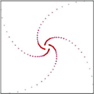
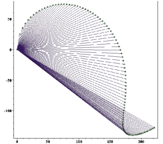
In order to illustrate the approach, we have shown the probabilistic images of a chain (1D-lattice of $N=100$ nodes) (see Fig. 2(1,2)), a polyhedron (a cycle of $N=50$ nodes) (see Fig. 2(3,4)), and a 2D-lattice $\mathcal{L}_{2}$ containing $10^{2}$ nodes (see Fig. 3). We suppose that all weights are equal $w_{xy}=1$, so that the respective affinity matrices are just the adjacency matrices of the graphs.

Random walks defined on the above networks embed them into the $(N-1)$-dimensional locus of Euclidean space, in which all nodes acquire certain norms quantified by the first-passage times to them from randomly chosen nodes. Indeed, the structure of $(N-1)$-dimensional vector spaces induced by random walks cannot be represented visually.

In order to obtain a 3D visual representation of these graphs, we have calculated their three major eigenvectors $\{\psi_{2},\psi_{3},\psi_{4}\},$ belonging to the largest eigenvalues $\mu_{k}<1$ of the symmetric transition operators (6). The $({\bf e}_{1},{\bf e}_{2},{\bf e}_{3})$-coordinates of the vertex $x\in V$ of the graph in 3D space have been taken equal to the relevant $x^{\mathrm{th}}$-components of three eigenvectors $\{\psi_{2},\psi_{3},\psi_{4}\}$. The radiuses of balls representing nodes in Figs. 2,3 have been taken proportional to the degrees of nodes. In Figs. 2.(1,3) and in Fig. 3(1), we have presented the the 3D images of the the chain, polyhedron , and the lattice $\mathcal{L}_{2}$. The connections between nodes represent the actual connections between them in the real space.

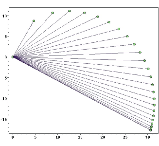
If we choose one node of a graph as a point of reference, we can draw the 2-dimensional projection of the $(N-1)$-dimensional locus by arranging other nodes at the distances calculated accordingly to (18) and under the angles (15) they are with respect to the chosen reference node. The examples are given in Fig.2(2,4).

In particular, in Fig.2(2), we have presented the 2-dimensional projection of the 99-dimensional Euclidean locus for a chain with respect to the marginal left node. The probabilistic Euclidean distance measured by the commute time (18) from the left end node is increasing node by node approximately as $\propto\sqrt{N}$ from $18.166$ random steps for the nearest neighbor node to $180.748$ random steps for the node at the opposite end of the chain ($x=100$). In Fig.2(4), the similar diagram is represented for the polyhedron. It is worth to mention that the symmetry of the polyhedron can also be seen in the image of its $49-$dimensional probabilistic locus. Chosen a vertex of the polyhedron as the reference node, the commute time with its nearest neighbors equals $9.899$ random steps, while it takes in average $35.355$ random steps in order to commute with the vertex on the circumcircle diametrically opposite to the origin.

In Fig.3(2), we have shown the matrix plot of the probabilistic Euclidean distances (the commute times) between all nodes of the lattice $\mathcal{L}_{2}$. The distances on the diagonal $d(x,x)=0$, and vary harmonically from 15 to 30 random steps for different pairs of nodes.

8 Acknowledgment

This work has been supported by the Volkswagen Foundation (Germany) in the framework of the project ”Network formation rules, random set graphs and generalized epidemic processes” (Contract no Az.: I/82 418).

References

- [1] H. Busemann, P.J. Kelly, Projectvie Geometry and Projective Metrics, in Pure and Applied Mathematics 3 (eds.) P.A.Smith, S. Eilenberg, Academic Press Inc., Publishers NY (1953).
- [2] D. Zwillinger, (Ed.). Affine Transformations. 4.3.2 in CRC Standard Mathematical Tables and Formulae. Boca Raton, FL: CRC Press, pp. 265-266 (1995).
- [3] Lovász, L. 1993 Random Walks On Graphs: A Survey. Bolyai Society Mathematical Studies 2: Combinatorics, Paul Erdös is Eighty, Keszthely (Hungary), p. 1-46.
- [4] Aldous,D.J., Fill, J.A. Reversible Markov Chains and Random Walks on Graphs. A book in preparation, available at www.stat.berkeley.edu/aldous/book.html.
- [5] Ph. Blanchard, D. Volchenkov, ”Intelligibility and first passage times in complex urban networks”, Proc. R. Soc. A doi:10.1098/rspa.2007.0329 (to be published in 2008).
- [6] Chung, F. 1997 Lecture notes on spectral graph theory, AMS Publications Providence.
- [7] D. Burago, Yu. Burago, S. Ivanov, A Course in Metric Geometry, Graduate Studies in Mathematics 33, AMS (2001).
- [8] Horn, R.A., Johnson, C.R., 1990 Matrix Analysis(chapter 8), Cambridge University Press.
- [9] A. Möbius, Der barycentrische Calcul (1827).