Smoothed Particle Hydrodynamics in Thermal Phases of a One Dimensional Molecular Cloud

Abstract

We present an investigation on effect of the ion-neutral (or ambipolar) diffusion heating rate on thermal phases of a molecular cloud. We use the modeling of ambipolar diffusion with two-fluid smoothed particle hydrodynamics, as discussed by Nejad-Asghar & Molteni. We take into account the ambipolar drift heating rate on the net cooling function of the molecular clouds, and we investigate the thermal phases in a self-gravitating magnetized one dimensional slab. The results show that the isobaric thermal instability criterion is satisfied in the outer parts of the cloud, thus, these regions are thermally unstable while the inner part is stable. This feature may be responsible for the planet formation in the outer parts of a collapsing molecular cloud and/or may also be relevant for the formation of star forming dense cores in the clumps.

I Introduction

In most plasmas, the forces acting on the ions are different from those acting on the electrons, so naively one would expect one species to be transported faster than the other, by diffusion or convection or some other process. If such differential transport has a divergence, then it will result in a change of the charge density, which will in turn create an electric field that will alter the transport of one or both species in such a way that they become equal. In astrophysics, ambipolar diffusion refers specifically to the decoupling of neutral particles from plasma. The neutral particles in this case are mostly hydrogen molecules in a cloud, and the plasma is composed of ions (mostly protons) and electrons, which are tied to the interstellar magnetic field.

Nejad-Asghar (2007) has recently made the assumption that the molecular cloud is initially an uniform ensemble which then fragments due to thermal instability. He finds that ambipolar drift heating is inversely proportional to density and its value, in outer parts of the cloud, can be significantly larger than the average heating rates of cosmic rays and turbulent motions. His results show that the isobaric thermal instability can occur in outer regions of the cloud. The rapid growth of thermal instability results a strong density imbalance between the cloud and the low-density surroundings; therefore it may produce the cloud fragmentation and formation of the condensations.

Many authors have developed computer codes that attempt to model ambipolar diffusion. Black & Scott (1982) used a two-dimensional, deformable-grid algorithm to follow the collapse of isothermal, non-rotating magnetized cloud. The three-dimensional work of MacLow et al. (1995) treats the two-fluid model in a version of the zeus magnetohydrodynamic code. An algorithm capable of using the smoothed particle hydrodynamics (SPH) to implement the ambipolar diffusion in a fully three-dimensional, self-gravitating system was developed by Hosking & Whitworth (2004). They described the SPH implementation of two-fluid technique that was tested by modeling the evolution of a dense core, which is initially thermally supercritical but magnetically subcritical. Nejad-Asghar & Molteni (2007) have recently optimized the two-fluid SPH implementation to test the pioneer works on the behavior of the ambipolar diffusion in an isothermal self-gravitating molecular layer.

In this paper, we include the SPH equivalent of the energy equation, which follows from the first law of thermodynamics. Here, we include the ambipolar drift heating rate in the net cooling function, and we investigate the thermal phases in the self-gravitating magnetized molecular layer. For this purpose, the two-fluid SPH technique and its algorithm are given in section 2. Section 3 devotes to the basic equations of the one dimensional molecular layer and its evolution by SPH. The summary and conclusion are presented in section 4.

II Numerical method

In two-fluid SPH technique of Hosking & Whitworth (2004), the initial SPH particles represent by two sets of molecular particles: magnetized ion SPH particles and non-magnetized neutral SPH particles. In this method, for each SPH particle we must create two separate neighbor lists: one for neighbors of the same species and another for those of different species. Consequently, each particle has two different smoothing lengths. In the following sections we refer to neutral particles as $\alpha$ and $\beta$, and ion particles as $a$ and $b$; the subscripts $1$ and $2$ refer to both ions and neutral particles. We adopt the usual smoothing spline-based kernel (Monaghan & Lattanzio 1985) and apply the symmetrized form proposed by Hernquist & Katz (1989)

$$W_{12}=W(\mid\textbf{r}_{1}-\textbf{r}_{2}\mid,h_{12})$$ (1)

where $\textbf{r}_{1}$, $\textbf{r}_{2}$ are positions of the particles $1$ and $2$, respectively. $h_{12}$ is the smoothing length of particle $1$ when considering neighbors of kind $2$. We update the adaptive smoothing length according to the octal-tree based nearest neighbor search algorithm (NNS).

The exact fraction of the total fluid that is ionized depends upon many factors (e.g. the neutral density, the cosmic ray ionization rate, how efficiently ionized metals are depleted on to dust grains). Here, we use the expression employed by Fiedler & Mouschovias (1992), which states that for $10^{8}<n<10^{15}\mathrm{m}^{-3}$,

$$\rho_{i}=\epsilon(\rho^{1/2}+\epsilon^{\prime}\rho^{-2}),$$ (2)

where in standard ionized equilibrium state, $\epsilon\sim 7.5\times 10^{-15}\mathrm{kg^{1/2}.m^{-3/2}}$ and $\epsilon^{\prime}\sim 4\times 10^{-44}\mathrm{kg^{5/2}.m^{-15/2}}$ are valid. In reality, the gas in this case is very weakly ionized, thus, we adopt the approximation $\rho=\rho_{n}+\rho_{i}\approx\rho_{n}$ in fluid equations. In this case, the molecular cloud is considered as global neutral which consists of a mixture of atomic and molecular hydrogen (with mass fraction $X$), helium (with mass fraction $Y$), and traces of $\mathrm{CO}$ and other rare molecules, thus, the mean molecular weight is given by $1/\mu=X/2+Y/4$.

The neutral density in place of neutral particles is estimated via usual summation over neighboring neutral particles

$$\rho_{n,\alpha}=\sum_{\beta}m_{\beta}W_{\alpha\beta},$$ (3)

while in place of ions, $\rho_{n,a}$, is given by interpolation technique from the values of the nearest neighbors. The ion density is evaluated via equation (2) as follows

$$\rho_{i,1}=1.8\times 10^{-9}\rho_{n,1}^{1/2}(1+3.5\times 10^{-17}\rho_{n,1}^{-5/2}),$$ (4)

for both places of ions and neutral particles. According to this new ion density, we update the mass of ion $a$ as

$$m_{a}^{new}=m_{a}^{old}\frac{\rho_{a}^{new}}{\rho_{a}^{old}},$$ (5)

in each time step so that the usual summation law

$$\rho_{i,a}=\sum_{\beta}m_{b}W_{ab},$$ (6)

for ions might being appropriate.

The SPH form of the drift velocity of ion particle $a$ is given by Hosking & Whitworth (2004) as

$$v_{d,a}=\frac{1}{\gamma_{AD}\rho_{n,a}}[-\frac{1}{\mu_{0}\rho_{i,a}}\sum_{b}\frac{m_{b}}{\rho_{i,b}}B_{b}B_{a}\frac{dW_{ab}}{dz_{a}}~{}~{}~{}~{}~{}~{}~{}~{}$$

$$-\sum_{b}m_{b}\Pi_{ab}\frac{dW_{ab}}{dz_{a}}].$$ (7)

where $\Pi_{ab}$ is the artificial viscosity between ion particles $a$ and $b$

$$\Pi_{ab}=\cases{\frac{\alpha^{*}a_{ab}\mu_{ab}+\beta^{*}\mu_{ab}^{2}}{\bar{\rho}_{ab}},&if $\textbf{v}_{ab}.\textbf{r}_{ab}<0$,\cr 0,&otherwise,}$$ (8)

where $\bar{\rho}_{ab}=\frac{1}{2}(\rho_{a}+\rho_{b})$ is an average density, $\alpha^{*}\sim 1$ and $\beta^{*}\sim 2$ are the coefficients, $a_{ab}=\frac{1}{2}(a_{a}+a_{b})$ is the mean sound speed, and $\mu_{ab}$ is defined as its usual form

$$\mu_{ab}=-\frac{\textbf{v}_{ab}\cdot\textbf{r}_{ab}}{\bar{h}_{ab}}\frac{1}{r_{ab}^{2}/\bar{h}_{ab}^{2}+0.001}$$ (9)

with $\bar{h}_{ab}=\frac{1}{2}(h_{a}+h_{b})$. Nejad-Asghar, Khesali & Soltani (2008) has recently considered the coefficients in the Monaghan’s standard artificial viscosity as time variable, and a restriction on them is proposed such that avoiding the undesired effects in the subsonic regions. Here, we use the Monaghan’s standard artificial viscosity, since the cloud contraction is quasi-hydrostatic and there is not supersonic motions and shock formation during this contraction.

It is better to keep in mind the second golden rule of SPH which is to rewrite formulae with the density inside operators (Monaghan 1992). In this case, the drift velocity is interpolated as

$$v_{d,a}=\frac{1}{\gamma_{AD}\rho_{n,a}}[-\frac{1}{2\mu_{0}\rho_{i,a}}\sum_{b}\frac{m_{b}}{\rho_{i,b}}(B_{b}^{2}-B_{a}^{2})\frac{dW_{ab}}{dz_{a}}~{}~{}$$

$$-\rho_{i,a}\sum_{b}\frac{m_{b}}{\rho_{i,b}}\Pi_{ab}\frac{dW_{ab}}{dz_{a}}],$$ (10)

where two extra density terms are introduced, one outside and one inside the summation sign. This comes as a result of the approximation to the volume integral needed to perform function interpolation (Nejad-Asghar & Molteni 2007).

There is no analytical expression that allows to calculate the value of drift velocity of the neutral particles. Here, we use the interpolation technique that starts at the nearest neighbor, then add a sequence of decreasing corrections, as information from other neighbors is incorporated (e.g., Press et al. 1992). These drift velocities at neutral places are used to estimate the drag acceleration

$$a_{drag,\alpha}=\gamma_{AD}\rho_{i,\alpha}v_{d,\alpha},$$ (11)

instead the method of Hosking & Whitworth (2004) who used the expression of Monaghan & Kocharayan (1995). In the usual symmetric form, the self-gravitating SPH acceleration equation for neutral particle $\alpha$ is

$$\frac{dv_{\alpha}}{dt}=g_{\alpha}-\sum_{\beta}m_{\beta}(\frac{p_{\alpha}}{\rho^{2}_{\alpha}}+\frac{p_{\beta}}{\rho^{2}_{\beta}}+\Pi_{\alpha\beta})\frac{dW_{\alpha\beta}}{dz_{\alpha}}+a_{drag,\alpha}$$ (12)

where $g_{\alpha}$ is the gravitational acceleration of particle $\alpha$.

The ion momentum equation assuming instantaneous velocity update so that we have

$$v_{a}=\sum_{\beta}\frac{m_{\beta}}{\rho_{\beta}}v_{\beta}W_{a\beta}+v_{d,a}$$ (13)

where the first term on the right-hand side gives the neutral velocity field at the ion particle $a$, calculated using a standard SPH approximation. Finally, the magnetic induction equation in SPH is

$$\frac{dB_{a}}{dt}=\sum_{b}\frac{m_{b}}{\rho_{b}}B_{a}v_{ab}\frac{dW_{ab}}{dz_{a}}.$$ (14)

where the usual notation is used.

In ambipolar diffusion process, the ion particles are physically diffused through the neutral fluid, thus, the ions will be bared in the boundary regions of the cloud (i.e. without any neutral particles in their neighbors). We check the position of ions before making a tree and nearest neighbor search, so that we send out the bared ion particles in the boundary regions of the simulation at next time-step. Both the cloud and boundary regions contain ion and neutral particles. We set up boundary particles ($4h_{1}$ up and down in $z$) using the linear extrapolation approach (from the values of the inner particles) to attribute the appropriate drift velocity, drag acceleration, pressure acceleration, and the magnetic induction rate to the boundary particles. The algorithm of the two-fluid SPH for simulation of thermal phases in a one dimensional molecular cloud is shown in Fig. 1.

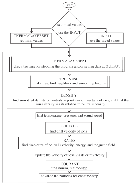
Figure 1: Algorithm of the two-fluid smoothed particle hydrodynamics for simulation of thermal phases in a one dimensional molecular cloud.

III layer evolution

III-A basic equations

We write the continuity equation of neutral part as its common form

$$\frac{d\rho}{dt}=-\rho\frac{\partial v}{\partial z},$$ (15)

while, the relation (2) is used to determine the ion density wherever it is required in the two-fluid equations. The momentum equation of neutral part then becomes

$$\frac{dv}{dt}=g-\frac{1}{\rho}\frac{\partial}{\partial z}(p+\frac{B^{2}}{2\mu_{0}})$$ (16)

where the gravitational acceleration $g$ obeys the poisson’s equation

$$\frac{\partial g}{\partial z}=-4\pi G\rho,$$ (17)

and the pressure is given by the ideal gas equation of state

$$p=\frac{k_{B}}{\mu m_{\mathrm{H}}}\rho T$$ (18)

where $m_{\mathrm{H}}$ is the mass of hydrogen atom and the temperature $T$ is approximated the same as for both neutral and ion fluids ($T_{i}=T_{n}=T$).

The thermal energy per unit mass is

$$u(T)=(\frac{5}{4}X+\frac{3}{8}Y)\frac{k_{B}T}{m_{H}}$$ (19)

where the mean internal (rotation and vibration) energy of an $\mathrm{H_{2}}$ molecule is included. The energy equation follows from the first law of thermodynamics, that is

$$\frac{du}{dt}=-\frac{p}{\rho}\frac{\partial v}{\partial z}-\Omega_{(\rho,T)},$$ (20)

where $\Omega_{(\rho,T)}$ is the net cooling function

$$\Omega_{(\rho,T)}\equiv\Lambda_{(n)}(\frac{T}{10\mathrm{K}})^{\beta_{(n)}}-(\Gamma_{CR}+\Gamma_{AD}),$$ (21)

where $\Gamma_{CR}$ and $\Gamma_{AD}$ are the heating rates due to cosmic rays and ambipolar diffusion, respectively, and $\Lambda_{(n)}$ and $\beta_{(n)}$ are the parameters for the gas cooling function that here we use the polynomial fitting functions, outlined by Nejad-Asghar (2007), as follows

$$\log\left(\frac{\Lambda_{(n)}}{\mathrm{J.kg^{-1}.s^{-1}}}\right)=-8.98-0.87(\log\frac{n}{n_{0}})$$

$$-0.14(\log\frac{n}{n_{0}})^{2},$$ (22)

$$\beta_{(n)}=3.07-0.11(\log\frac{n}{n_{0}})-0.13(\log\frac{n}{n_{0}})^{2},$$ (23)

where $n_{0}=10^{12}\mathrm{m^{-3}}$.

The magnetic fields are directly evolved by charged fluid component, as follows:

$$\frac{dB}{dt}=-B\frac{\partial v}{\partial z}+\frac{\partial}{\partial z}(Bv_{d}),$$ (24)

where the last term outlines the ambipolar diffusion effect with drift velocity,

$$v_{d}=-\frac{1}{\gamma_{AD}\epsilon\rho\rho_{i}}\frac{\partial}{\partial z}(\frac{B^{2}}{2\mu_{0}}),$$ (25)

which is obtained by assumption that the pressure and gravitational force on the charged fluid component are negligible compared to the Lorentz force because of the low ionization fraction. The notation $\gamma_{AD}\sim 3.5\times 10^{10}\mathrm{m^{3}/kg.s}$ in drift velocity represents the collision drag coefficient.

III-B results

The chosen physical scales for length and time are $[l]=200\mathrm{AU}$, and $[t]=10^{3}\mathrm{yr}$, respectively, so that velocity unit is approximately $[v]=1\mathrm{km.s^{-1}}$. The Newtonian constant of gravitation is set $G=1[m]^{-1}[l]^{3}[t]^{-2}$ for which the calculated mass unit is $[m]=4.5\times 10^{29}\mathrm{kg}$. Consequently, the derived physical scale for density, energy per unit mass, and drag coefficient are $[\rho]=1.7\times 10^{-11}\mathrm{kg.m^{-3}}$, $[u]=10^{6}\mathrm{J.kg^{-1}}$, and $\gamma_{AD}=1.8\times 10^{10}[l]^{3}[m]^{-1}[t]^{-1}$, respectively. In this manner, the numerical values of $\epsilon$ and $\epsilon^{\prime}$ are $1.8\times 10^{-9}[l]^{-3/2}[m]^{1/2}$ and $3.5\times 10^{-17}[l]^{-15/2}[m]^{5/2}$, respectively. The magnetic field is scaled in units such that the constant $\mu_{0}$ is unity. Since the magnetic flux density has dimensions

$$[B]=\frac{[m]}{[t][charge]},$$ (26)

while $\mu_{0}$ has dimensions

$$[\mu_{0}]=\frac{[m][l]}{[charge]^{2}},$$ (27)

specifying $\mu_{0}=1$ therefore scales the magnetic field equal to $[B]=5.1\mathrm{nT}$. With aforementioned units, the thermal energy per unit mass (19) is represented by $8.3\times 10^{-3}(5X/4+3Y/8)T$, the heating rates due to cosmic rays and ambipolar diffusion are $\Gamma_{CR}=1.1\times 10^{-3}[u]/[t]$ and

$$\Gamma_{AD,\alpha}=\gamma_{AD}\rho_{i,\alpha}v_{d,\alpha}^{2},$$ (28)

respectively, and the parameters for the gas cooling function are

$$\log\left(\frac{\Lambda_{\alpha}}{[u]/[t]}\right)=-4.48-0.87(\log\frac{\rho_{\alpha}}{2.24\times 10^{-4}})$$

$$-0.14(\log\frac{\rho_{\alpha}}{2.24\times 10^{-4}})^{2},$$ (29)

$$\beta_{\alpha}=3.07-0.11(\log\frac{\rho_{\alpha}}{2.24\times 10^{-4}})$$

$$-0.13(\log\frac{\rho_{\alpha}}{2.24\times 10^{-4}})^{2}.$$ (30)

The initial conditions for this simulation are a parallel magnetic field directed perpendicular to the $z$-axis so that the initial ratio of magnetic to gas pressure is everywhere a constant ($\alpha_{0}=1$), and a density profile given by

$$\rho=\frac{\rho_{0}}{\cosh^{2}(z/z_{\infty})}$$ (31)

where $\rho_{0}$ is the initial central density and $z_{\infty}\equiv c_{s}\sqrt{(1+\alpha_{0})/2\pi G\rho_{0}}$ is a length-scale parameter according to the initial sound speed $c_{s}$ (see Fig. 1 of Nejad-Asghar & Molteni 2007). The magnetic field is assumed to be frozen in the fluid of charged particles and the central density is assumed to be $\rho_{0}=2.24\times 10^{-4}[\rho]$. We choose a molecular cloud with the mass fraction of molecular hydrogen and helium are $X=0.75$ and $Y=0.25$, respectively, and have initial uniform temperature of $T_{0}=50\mathrm{K}$. We assume that the cloud layer is spread from $z=-93.2[l]$ to $z=+93.2[l]$ (according to Fig. 1 of Nejad-Asghar & Molteni 2007). The initial values of the cooling and heating functions are shown in Figure 2a. As presented in this figure, the isobaric thermal instability criterion,

$$\frac{\partial\Lambda}{\partial\rho}>\frac{\partial\Gamma}{\partial\rho},$$ (32)

is satisfied in the outer parts of the cloud, thus, these regions are thermally unstable while the inner part is stable as outlined by Nejad-Asghar (2007).

The present SPH code has the main features of the TreeSPH class so that the nearest neighbors searching are calculated by means of this procedure. We integrate the SPH equations using the one order simple integration scheme. The selection of time-step, $\Delta t$, is of great importance. There are several time-scales that can be defined locally in the system. For each particle $1$, we calculate the smallest of these time-scales using its smallest smoothing length, $h_{1}$, i.e.

$$\Delta t_{1}=C_{cour}\min[\frac{h_{1}}{|v_{1}|},\frac{h_{1}}{v_{A,1}},\frac{h_{1}}{a_{1}}],$$ (33)

where $v_{A}=B/\sqrt{\mu_{0}\rho_{i}}$ is the Alfvén speed of ion fluid and $C_{cour}$ is the Courant number which in this paper is adopted equal to $0.3$ (for numerical stability). The evolution were carried out to time $<u>/<\Lambda,\Gamma>\sim 0.43/0.025=17.2[t]$ so that the stability of the outer parts of the cloud may be revealed. The values of the cooling and heating rates versus position (and neutral density) are shown in Fig. 2b-d, at times $t=3.5[t]$, $10.5[t]$ and $17.2[t]$, respectively.

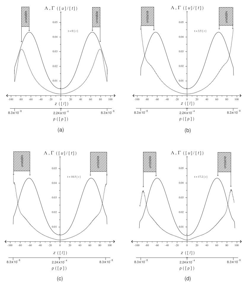
Figure 2: The values of the cooling (solid) and heating (dash) functions versus position (and neutral density), at initial time and $t=3.5[t]$, $10.5[t]$ and $17.2[t]$, respectively. Thermal unstable regions are shaded in this figure.

IV Summary and conclusions

In the preceding work of Nejad-Asghar & Molteni (2007), two-fluid SPH implementation was used to check the pioneer works on behavior of the ambipolar diffusion in an isothermal self-gravitating layer. In this paper, we include the SPH equivalent of the energy equation that can be obtained from the first law of thermodynamics. Here, we incorporate the ambipolar drift heating in the net cooling function, and we investigate the thermal phases in the self-gravitating magnetized molecular layer.

The values of the cooling and heating functions are shown in Figure 2. According to this figure, the isobaric thermal instability criterion is satisfied in the outer parts of the cloud, thus, these regions are thermally unstable while the inner part is stable. The SPH equations were integrated, and the evolution were carried out to time $17.2[t]$ so that the stability of the outer parts of the cloud is revealed.

It is obvious that the instability of the cloud at the outer parts, causes the formation two relative cool regions in that area. The rapid growth of thermal instability results a strong density imbalance between the cloud and the low-density surroundings. This feature may be responsible for the planet formation in the outer parts of a collapsing molecular cloud and/or may also be conscientious for the formation of star forming dense cores in the clumps.

References

- [1] D.C. Black and H. Scott, Astrophys. J., vol. 263, p. 696, 1982.
- [2] R.A. Fiedler and T.C. Mouschovias, Astrophys. J., vol. 391, p. 199, 1992.
- [3] L. Hernquist and N. Katz, Astrophys. J. Sup., vol. 70, p. 419, 1989.
- [4] J.G. Hosking and A.P. Whitworth, Mon. Not. Royal Aston. Soc., vol. 347, p. 994, 2004.
- [5] M.M. MacLow, M.L. Norman, A. Konigl and M. Wardle, Astrophys. J., vol. 442, p. 726, 1995.
- [6] J.J. Monaghan, Ann. Rev. Astron. Astrophys., vol. 30, p. 543, 1992.
- [7] J.J. Monaghan and A. Kocharyan, Comp. Phys. Commun., vol. 87, p. 225, 1995.
- [8] J.J. Monaghan and J.C. Lattanzio, Astron. Astrophys., vol. 149, p. 135, 1985.
- [9] M. Nejad-Asghar, Mon. Not. Royal Aston. Soc., vol. 379, p. 222, 2007.
- [10] M. Nejad-Asghar and D. Molteni, Joint Eroup. National Astron. Meeting, Yerevan, Armenia, 20-25 August, 2007, asto-ph0802.2437.
- [11] M. Nejad-Asghar, A.R. Khesali and J. Soltani, Astophys. Space Sci., vol. 313, p. 425, 2008.