Abstract

In this article, we study the final-state rescattering effects in the decay $B^{0}\to\eta_{c}K^{*}$, the numerical results indicate the corrections are comparable with the contribution from the naive factorizable amplitude, and the total amplitudes can accommodate the experimental data.

PACS numbers: 13.20.He; 14.40.Lb

Key Words: Final-state interactions, $B$-decay

1 Introduction

The nonleptonic decays of the $B$ meson have attracted much attention in studying the nonperturbative dynamics of QCD, final-state interactions and CP violation. The exclusive $B$ to charmonia decays are of great importance since the decays $B\to J/\psi K,\eta_{c}K,\chi_{cJ}K$ are regarded as the golden channels for studying CP violation. The quantitative understanding of those decays depends on our knowledge about the nonperturbative hadronic matrix elements of the operators entering the effective weak Hamiltonian. The $B$ factories (BaBar, Belle, etc) have measured the color-suppressed decays to a charmonium and a $K$ (or $K^{*}$) meson with relatively large branching fractions [1], for examples, $\rm{Br}(B^{0}\to J/\psi K^{0})=(8.72\pm 0.33)\times 10^{-4}$, $\rm{Br}(B^{+}\to J/\psi K^{+})=(10.07\pm 0.35)\times 10^{-4}$, $\rm{Br}(B^{0}\to\eta_{c}K^{0})=(9.9\pm 1.9)\times 10^{-4}$, $\rm{Br}(B^{+}\to\eta_{c}K^{+})=(9.1\pm 1.3)\times 10^{-4}$, $\rm{Br}(B^{0}\to\eta_{c}K^{*0})=(1.6\pm 0.7)\times 10^{-3}$, etc, which take place through the process $b\to sc\bar{c}$ (or more precise $\bar{b}\to\bar{s}c\bar{c}$, they relate with each other by charge conjunction, in this article, we calculate the amplitudes for the process $b\to sc\bar{c}$, then take charge conjunction to obtain the branching fraction.) at the quark-level.

Recently, the BaBar Collaboration measured the processes $B^{0}\to\eta_{c}K^{*0}$, $B^{0}\to\eta_{c}(2S)K^{*0}$, $B^{0}\to h_{c}K^{*0}$, $B^{+}\to h_{c}K^{+}$ and $\eta_{c}(2S)\to K\bar{K}\pi$ from the $B$-decays to $(K\bar{K}\pi)K^{+}$, $(K\bar{K}\pi)K^{*0}$, $\eta_{c}\gamma K^{+}$ and $\eta_{c}\gamma K^{*0}$. The branching fractions are $\rm{Br}(B^{0}\to\eta_{c}K^{*0})=(5.7\pm 0.6\pm 0.9)\times 10^{-4}$, $\rm{Br}(B^{0}\to\eta_{c}(2S)K^{*0})<3.9\times 10^{-4}$, $\rm{Br}(B^{+}\to h_{c}K^{+})\rm{Br}(h_{c}\to\eta_{c}\gamma)<4.8\times 10^{-5}$ and $\rm{Br}(B^{0}\to h_{c}K^{*0})\rm{Br}(h_{c}\to\eta_{c}\gamma)<2.2\times 10^{-4}$ at the $90\%$ C.L. [2].

The decays $B\rightarrow J/\psi K,\eta_{c}K,\chi_{cJ}K$ have been calculated with the QCD-improved factorization approach [3, 4], there are infrared divergence in vertex corrections and logarithmical divergence in spectator corrections beyond the leading twist approximation for the $S$-wave charmonia and in the leading twist approximation for the $P$-wave charmonia, moreover, the predicted branching fractions are too small to accommodate the experimental data [5, 6, 7, 8, 9, 10]. The decay $B\rightarrow J/\psi K^{*}$ has also been studied with the QCD-improved factorization approach, the factorization breaks down even at the twist-2 level for transverse hard spectator interactions [11].

In Refs.[12, 13, 14], the soft nonfactorizable contributions in the decays $B\to J/\psi K,\chi_{c0}K,\chi_{c1}K,\eta_{c}K$ are studied with the light-cone QCD sum rules, the predicted small branching fractions cannot accommodate the (relatively large) experimental data.

In Ref.[15], the authors study the decays $B\to J/\psi K$, $\chi_{c0}K$, $\chi_{c1}K$, $\eta_{c}K$, $J/\psi K^{*}$, $\chi_{c0}K^{*}$, $\chi_{c1}K^{*}$, $\eta_{c}K^{*}$ with the perturbative QCD approach based on $k_{T}$ factorization theorem, and the branching fractions $\rm{Br}(B\to\eta_{c}K)$ and $\rm{Br}(B^{0}\to\eta_{c}K^{*0})$ ($2.64^{+2.71}_{-2.58}\times 10^{-4}$) are too small to take into account the experimental data [2].

Final-state interactions play an important role in the hadronic $B$-decays, the color-suppressed neutral modes such as $B^{0}\to D^{0}\pi^{0},\pi^{0}\pi^{0},\rho^{0}\pi^{0},K^{0}\pi^{0}$ are enhanced substantially by the long-distance rescattering effects [16]. In Refs.[17, 18], the authors study the rescattering effects of the intermediate charmed mesons for the decays $B^{-}\to\chi_{c0}K^{-},h_{c}K^{-}$ and observe the final-state interactions can lead to larger branching fractions to account the experimental data. The factorizable amplitude in the decay $B^{0}\to\eta_{c}K^{*}$ is too small to accommodate the experimental data [2], so it is intersecting to study the effects of the final-state interactions.

The article is arranged as: in Section 2, we study the final-state rescattering effects in the decay $B^{0}\to\eta_{c}K^{*}$; in Section 3, the numerical result and discussion; and Section 4 is reserved for conclusion.

2 Final-state rescattering effects in the decay $B^{0}\to\eta_{c}K^{*}$

The effective weak Hamiltonian for the decay modes $b\rightarrow sc\bar{c}$ can be written as (for detailed discussion of the effective weak Hamiltonian, one can consult Ref.[19])

$$H_{w}=\frac{G_{F}}{\sqrt{2}}\left\{V_{cb}V_{cs}^{*}\left[C_{1}(\mu){\cal O}_{1}(\mu)+C_{2}(\mu){\cal O}_{2}(\mu)\right]-V_{tb}V_{ts}^{*}\sum_{i=3}^{10}C_{i}(\mu){\cal O}_{i}(\mu)\right\}\,,$$ (1)

where $V_{ij}$’s are the CKM matrix elements, $C_{i}$’s are the Wilson coefficients calculated at the renormalization scale $\mu\sim O(m_{b})$ and the relevant operators ${\cal O}_{i}$ are given by

$${\cal O}_{1} = (\overline{s}_{\alpha}b_{\alpha})_{V-A}(\overline{c}_{\beta}c_{\beta})_{V-A}\,,$$

$${\cal O}_{2} = (\overline{s}_{\alpha}b_{\beta})_{V-A}(\overline{c}_{\beta}c_{\alpha})_{V-A}\,,$$

$${\cal O}_{3(5)} = (\overline{s}_{\alpha}b_{\alpha})_{V-A}\sum_{q}(\overline{q}_{\beta}q_{\beta})_{V-A(V+A)}\,,$$

$${\cal O}_{4(6)} = (\overline{s}_{\alpha}b_{\beta})_{V-A}\sum_{q}(\overline{q}_{\beta}q_{\alpha})_{V-A(V+A)}\,,$$

$${\cal O}_{7(9)} = {3\over 2}(\overline{s}_{\alpha}b_{\alpha})_{V-A}\sum_{q}e_{q}(\overline{q}_{\beta}q_{\beta})_{V+A(V-A)}\,,$$

$${\cal O}_{8(10)} = {3\over 2}(\overline{s}_{\alpha}b_{\beta})_{V-A}\sum_{q}e_{q}(\overline{q}_{\beta}q_{\alpha})_{V+A(V-A)}\,,$$ (2)

$\alpha$ and $\beta$ are color indexes. We can reorganize the color-mismatched quark fields into color singlet states by Fierz transformation (for example, ${\cal{O}}_{2}=\frac{1}{3}{\cal{O}}_{1}+2{\cal\widetilde{O}}_{1}$, ${\cal\widetilde{O}}_{1}=(\overline{s}\frac{\lambda^{a}}{2}b)_{V-A}(\overline{c}\frac{\lambda^{a}}{2}c)_{V-A}$, $\lambda^{a}$’s are the Gell-Mann matrices), and obtain the factorizable amplitude,

$$\langle\eta_{c}(p_{3})K^{*}(p_{4})|H_{w}|B(P)\rangle = \frac{G_{F}}{\sqrt{2}}\left\{V_{cb}V_{cs}^{*}(C_{1}+\frac{C_{2}}{3})-V_{tb}V_{ts}^{*}(C_{3}-C_{5}+\frac{C_{4}-C_{6}}{3})\right\}$$ (3)

$$\langle\eta_{c}(p_{3})|\overline{c}\gamma_{\mu}(1-\gamma_{5})c|0\rangle\langle K^{*}(p_{4})|\overline{s}\gamma^{\mu}(1-\gamma_{5})b|B(P)\rangle$$

$$= \frac{G_{F}}{\sqrt{2}}\left\{V_{cb}V_{cs}^{*}(C_{1}+\frac{C_{2}}{3})-V_{tb}V_{ts}^{*}(C_{3}-C_{5}+\frac{C_{4}-C_{6}}{3})\right\}$$

$$2P\cdot\epsilon^{*}_{4}f_{\eta_{c}}M_{K^{*}}A_{0}(p_{3}^{2})\,,$$

where we have used the standard definitions for the weak form-factors (we write down all form-factors to be used in this article) [20, 21],

$$\langle D(p)|\overline{s}\gamma_{\mu}(1-\gamma_{5})b|B(P)\rangle = (P+p)_{\mu}F_{1}(q^{2})-\frac{M_{B}^{2}-M_{D}^{2}}{q^{2}}q_{\mu}[F_{1}(q^{2})-F_{0}(q^{2})]\,,$$

$$\langle V(p)|\overline{s}\gamma_{\mu}(1-\gamma_{5})b|B(P)\rangle = i{\epsilon_{\mu}}^{\nu\alpha\beta}\epsilon^{*}_{\nu}P_{\alpha}p_{\beta}\frac{2V(q^{2})}{M_{B}+M_{V}}-\frac{2M_{V}q\cdot\epsilon^{*}}{q^{2}}q_{\mu}A_{0}(q^{2})$$ (4)

$$-\left[\epsilon_{\mu}^{*}-\frac{q\cdot\epsilon^{*}}{q^{2}}q_{\mu}\right](M_{B}+M_{V})A_{1}(q^{2})+$$

$$\left[(P+p)_{\mu}-\frac{M_{B}^{2}-M_{V}^{2}}{q^{2}}q_{\mu}\right]q\cdot\epsilon^{*}\frac{A_{2}(q^{2})}{M_{B}+M_{V}}\,,$$

the $\epsilon_{\mu}$ is the polarization vector of the vector meson and $q_{\mu}=P_{\mu}-p_{\mu}$. In this article, we use the value of the $B\to K^{*}$ form-factor $A_{0}(q^{2})$ from the light-cone QCD sum rules [22],

$$A_{0}(q^{2}) = \frac{1.364}{1-q^{2}/M_{B}^{2}}-\frac{0.990}{1-q^{2}/36.78}\,.$$ (5)

The factorizable amplitude (see Eq.(3)) at the tree level is too small to accommodate the experimental data.

The decays $B^{0}\to DD_{s}$, $DD_{s}^{*}$, $D^{*}D_{s}$, $D^{*}D_{s}^{*}$ are color enhanced due to the large Wilson coefficient $C_{2}$,

$$\langle D_{s}(q)D^{*}(p)|H_{w}|B(P)\rangle = \sqrt{2}G_{F}V_{cb}V_{cs}^{*}(C_{2}+\frac{C_{1}}{3})P\cdot\epsilon^{*}f_{D_{s}}M_{D^{*}}A_{0}(q^{2})\,,$$

$$\langle D_{s}^{*}(q)D(p)|H_{w}|B(P)\rangle = \sqrt{2}G_{F}V_{cb}V_{cs}^{*}(C_{2}+\frac{C_{1}}{3})P\cdot\epsilon^{*}f_{D_{s}^{*}}M_{D^{*}_{s}}F_{1}(q^{2})\,,$$ (6)

we write down only the amplitudes appear in the final expressions. In the heavy quark limit, the weak form-factors $A_{0}(q^{2})$ and $F_{1}(q^{2})$ can be related to the universal Isgur-Wise form-factor $\xi(\omega)$ [23],

$$F_{1}(q^{2}) = \frac{M_{B}+M_{D}}{2\sqrt{M_{B}M_{D}}}\xi\left(\frac{M_{B}^{2}+M_{D}^{2}-q^{2}}{2M_{B}M_{D}}\right)\,,$$

$$A_{0}(q^{2}) = \frac{M_{B}+M_{D^{*}}}{2\sqrt{M_{B}M_{D^{*}}}}\xi\left(\frac{M_{B}^{2}+M_{D^{*}}^{2}-q^{2}}{2M_{B}M_{D^{*}}}\right)\,,$$ (7)

where $\xi(\omega)=\left(\frac{2}{1+\omega}\right)^{2}$, which is compatible with the experimental data for the semileptonic decays $B\to D^{*}(D)l\nu_{l}$ [24].

The decay $B^{0}\to\eta_{c}K^{*}$ can also take place through the decay cascades $B^{0}\to DD_{s}$, $DD_{s}^{*}$, $D^{*}D_{s}$, $D^{*}D_{s}^{*}$ $\to\eta_{c}K^{*}$, the rescattering amplitudes of $DD_{s}$, $DD_{s}^{*}$, $D^{*}D_{s}$, $D^{*}D_{s}^{*}$ $\to\eta_{c}K^{*}$ may play an important role.

The final-state interactions can be described by the following effective lagrangians,

$$\mathcal{L}_{\eta_{c}D^{*}D} = -ig_{\eta_{c}D^{*}D}\eta_{c}\left[\partial^{\mu}D{D}_{\mu}^{*\dagger}-{D}_{\mu}^{*}\partial^{\mu}{D}^{\dagger}\right]\,,$$ (8)

$$\mathcal{L}_{\eta_{c}D^{*}D^{*}} = g_{\eta_{c}D^{*}D^{*}}\varepsilon^{\mu\nu\alpha\beta}\eta_{c}\partial_{\mu}{D}_{\nu}^{*\dagger}\partial_{\alpha}{D}_{\beta}^{*}\,,$$ (9)

$$\mathcal{L}_{DDV} = -ig_{DDV}D_{i}^{\dagger}{\stackrel{{\scriptstyle\leftrightarrow}}{{\partial}}}_{\mu}D^{j}(\mathbb{V}^{\mu})^{i}_{j}\,,$$ (10)

$$\mathcal{L}_{D^{*}DV} = -2f_{D^{*}DV}\varepsilon^{\mu\nu\alpha\beta}(\partial_{\mu}\mathbb{V}_{\nu})^{i}_{j}\left[D_{i}^{\dagger}{\stackrel{{\scriptstyle\leftrightarrow}}{{\partial}}}_{\alpha}D_{\beta}^{*j}-D^{*\dagger}_{\beta i}{\stackrel{{\scriptstyle\leftrightarrow}}{{\partial}}}_{\alpha}D^{j}\right]\,,$$ (11)

$$\mathcal{L}_{D^{*}D^{*}V} = ig_{D^{*}D^{*}V}D^{*\nu\dagger}_{i}{\stackrel{{\scriptstyle\leftrightarrow}}{{\partial}}}_{\mu}D^{*j}_{\nu}(\mathbb{V}^{\mu})^{i}_{j}+4if_{D^{*}D^{*}V}D^{*\dagger}_{i\mu}(\partial^{\mu}\mathbb{V}^{\nu}-\partial^{\nu}\mathbb{V}^{\mu})^{i}_{j}D^{*j}_{\nu}\,,$$ (12)

where the indexes $i,j$ stand for the flavors of the light quarks, $D^{(*)}$=$(\bar{D}^{(*)0}$, $D^{(*)-}$, $D_{s}^{(*)-})^{T}$, $\mathbb{V}$ is the $3\times 3$ matrix for the nonet vector mesons,

$$\mathbb{V} = \left(\begin{array}[]{ccc}\frac{\rho^{0}}{\sqrt{2}}+\frac{\omega}{\sqrt{2}}&\rho^{+}&K^{*+}\\ \rho^{-}&-\frac{\rho^{0}}{\sqrt{2}}+\frac{\omega}{\sqrt{2}}&K^{*0}\\ K^{*-}&\bar{K}^{*0}&\phi\end{array}\right).$$ (16)

The lagrangians $\mathcal{L}_{DDV}$, $\mathcal{L}_{D^{*}DV}$ and $\mathcal{L}_{D^{*}D^{*}V}$ are taken from Ref.[16], and the $\mathcal{L}_{\eta_{c}D^{*}D}$ and $\mathcal{L}_{\eta_{c}D^{*}D^{*}}$ are constructed from the heavy quark theory in this article. In the heavy quark limit, the strong coupling constants $f_{D^{*}DV}$, $f_{D^{*}D^{*}V}$, $g_{DDV}$ and $g_{D^{*}D^{*}V}$ can be related to the basic parameters $\lambda$ and $\beta$ in the heavy quark effective Lagrangian (one can consult Ref.[25] for the heavy quark effective lagrangian and relevant parameters, we neglect them for simplicity),

$$f_{D^{*}DV} = \frac{f_{D^{*}D^{*}V}}{M_{D^{*}}}=\frac{\lambda g_{V}}{\sqrt{2}}\,,$$

$$g_{DDV} = g_{D^{*}D^{*}V}=\frac{\beta g_{V}}{\sqrt{2}}\,,$$ (17)

where $g_{V}=5.8$ from the vector meson dominance theory [26]. The strong coupling constants $g_{\eta_{c}D^{*}D}$ and $g_{\eta_{c}D^{*}D^{*}}$ are estimated with the universal Isgur-Wise form-factor at zero recoil $\xi(1)$ and the assumption of dominance of the intermediate $\eta_{c}$ meson for the pseudoscalar heavy quark current $\overline{c}i\gamma_{5}c$,

$$g_{\eta_{c}D^{*}D} = \frac{2m_{c}}{f_{\eta_{c}}}\approx\frac{M_{\eta_{c}}}{f_{\eta_{c}}}\,,$$

$$g_{\eta_{c}D^{*}D^{*}} = \frac{g_{\eta_{c}D^{*}D}}{M_{D^{*}}}\,.$$ (18)

The rescattering effects can be taken into account by twelve Feynman diagrams, see Fig.1. We calculate the absorptive parts (or imaginary parts) of the rescattering amplitudes $\textbf{Abs}(i)$ by the Cutkosky rule, $\textbf{Abs}(i)=\widetilde{\textbf{Abs}}(i)\frac{G_{F}}{\sqrt{2}}V_{cb}V_{cs}^{*}(C_{2}+\frac{C_{1}}{3})$,

$$\widetilde{\textbf{Abs}}(a) = \frac{|\vec{p}_{1}|}{8\pi^{2}M_{B}}\int d\Omega\left[f_{D_{s}}M_{D^{*}}g_{\eta_{c}D^{*}D}g_{DDV}A_{0}(p_{2}^{2})\right]\frac{\mathcal{F}^{2}(M_{D},t)}{t-M_{D}^{2}}$$

$$p_{2}\cdot\epsilon_{4}^{*}p_{2}\cdot\epsilon_{1}^{*}q\cdot\epsilon_{1}\,,$$

$$\widetilde{\textbf{Abs}}(b) = \frac{|\vec{p}_{1}|}{8\pi^{2}M_{B}}\int d\Omega\left[f_{D_{s}^{*}}M_{D_{s}^{*}}g_{\eta_{c}D^{*}D}g_{DDV}F_{1}(p_{1}^{2})\right]\frac{\mathcal{F}^{2}(M_{D_{s}},t)}{t-M_{D_{s}}^{2}}$$

$$p_{2}\cdot\epsilon_{4}^{*}p_{2}\cdot\epsilon_{1}^{*}q\cdot\epsilon_{1}\,,$$

$$\widetilde{\textbf{Abs}}(c) = -\frac{|\vec{p}_{1}|}{4\pi^{2}M_{B}}\int d\Omega\left[f_{D_{s}}M_{D^{*}}g_{\eta_{c}D^{*}D^{*}}f_{D^{*}DV}A_{0}(p_{2}^{2})\right]\frac{\mathcal{F}^{2}(M_{D^{*}},t)}{t-M_{D^{*}}^{2}}$$

$$\epsilon^{\mu\nu\alpha\beta}\epsilon^{\mu^{\prime}\nu^{\prime}\alpha^{\prime}\beta}p_{4\mu}\epsilon_{4\nu}p_{2\alpha}p_{1\mu^{\prime}}p_{2\nu^{\prime}}q_{\alpha^{\prime}}\,,$$

$$\widetilde{\textbf{Abs}}(d) = -\frac{|\vec{p}_{1}|}{4\pi^{2}M_{B}}\int d\Omega\left[f_{D_{s}^{*}}M_{D^{*}_{s}}g_{\eta_{c}D^{*}D^{*}}f_{D^{*}DV}F_{1}(p_{1}^{2})\right]\frac{\mathcal{F}^{2}(M_{D^{*}_{s}},t)}{t-M_{D^{*}_{s}}^{2}}$$

$$\epsilon^{\mu\nu\alpha\beta}\epsilon^{\mu^{\prime}\beta\alpha^{\prime}\beta^{\prime}}p_{4\mu}\epsilon_{4\nu}p_{2\alpha}q_{\mu^{\prime}}p_{1\alpha^{\prime}}p_{2\beta^{\prime}}\,,$$

$$\widetilde{\textbf{Abs}}(e) = \frac{|\vec{p}_{1}|}{8\pi^{2}M_{B}}\int d\Omega\left[f_{D_{s}^{*}}M_{D^{*}_{s}}g_{\eta_{c}D^{*}D}F_{1}(p_{2}^{2})\right]\frac{\mathcal{F}^{2}(M_{D^{*}},t)}{t-M_{D^{*}}^{2}}$$

$$\left[-g_{D^{*}D^{*}V}p_{2}\cdot\epsilon_{4}^{*}p_{1}\cdot\epsilon^{*}(q)\epsilon(q)\cdot\epsilon_{2}p_{1}\cdot\epsilon^{*}_{2}\right.$$

$$-2f_{D^{*}D^{*}V}p_{4}\cdot\epsilon_{2}p_{1}\cdot\epsilon^{*}_{2}p_{1}\cdot\epsilon^{*}(q)\epsilon(q)\cdot\epsilon^{*}_{4}$$

$$\left.+2f_{D^{*}D^{*}V}p_{4}\cdot\epsilon(q)p_{1}\cdot\epsilon^{*}(q)p_{1}\cdot\epsilon^{*}_{2}\epsilon_{2}\cdot\epsilon^{*}_{4}\right]\,,$$

$$\widetilde{\textbf{Abs}}(f) = \frac{|\vec{p}_{1}|}{8\pi^{2}M_{B}}\int d\Omega\left[f_{D_{s}}M_{D^{*}}g_{\eta_{c}D^{*}D}A_{0}(p_{1}^{2})\right]\frac{\mathcal{F}^{2}(M_{D^{*}_{s}},t)}{t-M_{D^{*}_{s}}^{2}}$$

$$\left[-g_{D^{*}D^{*}V}p_{2}\cdot\epsilon_{4}^{*}p_{1}\cdot\epsilon^{*}(q)\epsilon(q)\cdot\epsilon_{2}p_{1}\cdot\epsilon^{*}_{2}\right.$$

$$-2f_{D^{*}D^{*}V}p_{4}\cdot\epsilon_{2}p_{1}\cdot\epsilon^{*}_{2}p_{1}\cdot\epsilon^{*}(q)\epsilon(q)\cdot\epsilon^{*}_{4}$$

$$\left.+2f_{D^{*}D^{*}V}p_{4}\cdot\epsilon(q)p_{1}\cdot\epsilon^{*}(q)p_{1}\cdot\epsilon^{*}_{2}\epsilon_{2}\cdot\epsilon^{*}_{4}\right]\,,$$

$$\widetilde{\textbf{Abs}}(g) = -\widetilde{\textbf{Abs}}(h)\,\,\text{ (in SU(3) limit})\,,$$

$$\widetilde{\textbf{Abs}}(i) = -\widetilde{\textbf{Abs}}(j)\,\,\text{ (in SU(3) limit})\,,$$

$$\widetilde{\textbf{Abs}}(k) = -\widetilde{\textbf{Abs}}(l)\,\,\text{ (in SU(3) limit})\,,$$ (19)

where $\vec{p}_{1}$ is the 3-momentum of the on-shell intermediate mesons $D,D^{*},D_{s},D_{s}^{*}$ in the rest frame of the $B$ meson, for example, in the process $B^{0}\to D^{*}(p_{1})D_{s}(p_{2})\to\eta_{c}(p_{3})K^{*}(p_{4})$, $t=q^{2}$, $q=p_{1}-p_{3}=p_{4}-p_{2}$, $\epsilon^{\mu}_{i}$ is the polarization vector of the vector meson $i$. The off-shell effects of the $t$-channel exchanged mesons $D$, $D^{*}$, $D_{s}$ and $D_{s}^{*}$ are taken into account by introducing a monopole form-factor [16],

$$\mathcal{F}(M_{i},t)=\frac{\Lambda_{i}^{2}-M_{i}^{2}}{\Lambda_{i}^{2}-t},$$ (20)

and the cutoff $\Lambda_{i}$ are parameterized as

$$\Lambda_{i}=M_{i}+\alpha\Lambda_{\rm{QCD}}\,,$$ (21)

where $\alpha$ is a free parameter and $\Lambda_{\rm{QCD}}=0.225\rm{GeV}$. In fact, the $g_{s}\mathcal{F}(M_{i},t)$ are the momentum dependent strong coupling constants, we can vary the parameter $\alpha$ to change the effective strong couplings, here we use the notation $g_{s}$ to denote all the strong coupling constants.

The dispersive parts (or real parts) of the rescattering amplitudes can be obtained via the dispersion relation,

$$\textbf{Dis}(i)(M_{B}^{2})={1\over\pi}\textbf{P}\int_{s_{th}}^{\infty}{\textbf{Abs}(i)(s^{\prime})\over s^{\prime}-M_{B}^{2}}ds^{\prime}\,,$$ (22)

where the thresholds $s_{th}$ are given by $s_{th}=(M_{D}+M_{D^{*}_{s}})^{2}$ , $(M_{D^{*}}+M_{D_{s}})^{2}$, $(M_{D}+M_{D_{s}})^{2}$, $(M_{D^{*}}+M_{D^{*}_{s}})^{2}$ for any specific diagram. There are large uncertainties due to the cut-off procedure, even one assume that the integrals are dominated by the region close to the pole $M_{B}^{2}$ [17, 18]. In this article, we assume the dominating contributions of the rescattering amplitudes come from the absorptive parts, which originate from the on-shell intermediate states in the decay cascades, the dispersive parts of the amplitudes are of minor importance and can be taken into account by introducing a phenomenological parameter $\rho$, $\textbf{Dis}(i)=\rho\textbf{Abs}(i)$, $\rho\leq 30\%$.

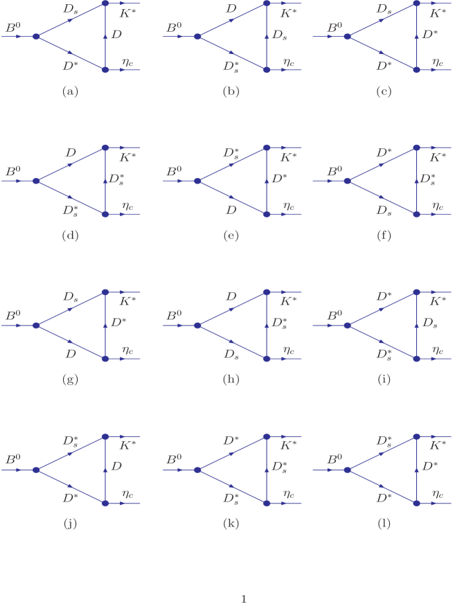
Figure 1: The Feynman diagrams for the final-state interactions.

3 Numerical result and discussions

The CKM matrix elements are taken as $V_{cs}=0.97296\pm 0.00024$, $V_{cb}=(41.6\pm 0.6)\times 10^{-3}$, $V_{tb}=0.999100^{+0.000034}_{-0.000004}$ and $V_{ts}=-(40.6\pm 2.7)\times 10^{-3}$ [1, 27]. We take the next-to-leading order Wilson coefficients calculated in the naive dimensional regularization scheme for $\mu=\overline{m_{b}}(m_{b})=4.40{\rm\,GeV}$ and $\Lambda_{\overline{\rm MS}}^{(5)}=225\,{\rm MeV}$, $C_{1}(\mu)=-0.185$, $C_{2}(\mu)=1.082$, $C_{3}(\mu)=0.014$, $C_{4}(\mu)=-0.035$, $C_{5}(\mu)=0.009$ and $C_{6}(\mu)=-0.041$ [19], here we have neglected the Wilson coefficients $C_{7},C_{8},C_{9},C_{10}$ in numerical calculation due to their small values. The masses of the mesons are taken as $M_{B}=5.279\,\rm{GeV}$, $M_{K^{*}}=0.892\,\rm{GeV}$, $M_{D}=1.87\,\rm{GeV}$, $M_{D_{s}}=1.97\,\rm{GeV}$, $M_{D^{*}}=2.010\,\rm{GeV}$ and $M_{D_{s}^{*}}=2.112\,\rm{GeV}$ [1], and $M_{\eta_{c}}=2.986\,\rm{GeV}$ [2].

The values of the decay constants $f_{D}$, $f_{D_{s}}$, $f_{D^{*}}$ and $f_{D^{*}_{s}}$ vary in a large range from different approaches, for examples, the potential model, QCD sum rules and lattice QCD, etc [30, 31, 32]. For the $f_{D}$, we take the experimental data from the CLEO Collaboration, $f_{D}=222.6\pm 16.7^{+2.8}_{-3.4}\,\,\rm{MeV}$ [33, 34]. The value $f_{D_{s}}=(0.274\pm 0.013)\,\rm{GeV}$ from the CLEO Collaboration shows the $SU(3)$ breaking effect is rather large [35], $\frac{f_{D_{s}}}{f_{D}}=1.23$, while most of theoretical calculations indicate $\frac{f_{D_{s}}}{f_{D}}\approx 1.1$, we take the value $f_{D^{*}}=f_{D}=(0.22\pm 0.02)\,\rm{GeV}$ and $f_{D^{*}_{s}}=f_{D_{s}}=(0.24\pm 0.02)\,\rm{GeV}$.

The decay constant $f_{\eta_{c}}$ can be estimated with the QCD sum rules [36] or phenomenological potential models, the values from those approaches are compatible with each other, we can take the value $f_{\eta_{c}}=(0.35\pm 0.02)\,\rm{GeV}$ [37, 38, 39].

The basic parameters $\lambda$ and $\beta$ in the heavy quark effective Lagrangian are estimated with the vector meson dominance theory [28, 29], $\lambda=0.56\,\rm{GeV}^{-1}$ and $\beta=0.9$. The corresponding values of the strong coupling constants are

$$f_{D^{*}DV} = 2.30\,\rm{GeV}^{-1}\,,$$

$$f_{D^{*}D^{*}V} = 4.61\,,$$

$$g_{DDV} = 3.69\,,$$

$$g_{D^{*}D^{*}V} = 3.69\,,$$ (23)

while the values from the light-cone QCD sum rules are much smaller [40, 41]. In this article, the strong coupling constants $g_{\eta_{c}D^{*}D}$ and $g_{\eta_{c}D^{*}D^{*}}$ are estimated with the universal Isgur-Wise form-factor at zero recoil $\xi(1)$ and the assumption of dominance of the intermediate $\eta_{c}$ meson for the pseudoscalar heavy quark current $\overline{c}i\gamma_{5}c$. We take the results from the vector meson dominance theory for consistence. However, we may overestimate the final-state rescattering effects due to the larger strong coupling constants, and have to compensate them with suitable $\alpha$.

The parameters $\alpha$ and $\rho$ are taken to be $\rho=0.3$, $\alpha=1.4-1.8$. The contributions from the rescattering effects are somewhat sensitive to the parameter $\alpha$ (or the constant $\Lambda_{i}$ in the form-factors), the $\Lambda_{i}$ is of the order of the mass of radial excitations of the charmed mesons [17, 18].

Finally we obtain the numerical results for the branching fractions,

$$\rm{Br}(B^{0}\to\eta_{c}K^{*}) = (3.25-4.09)\times 10^{-4}\,\,\,\text{(Tree amplitude)}\,,$$

$$\rm{Br}(B^{0}\to\eta_{c}K^{*}) = (3.90-5.31)\times 10^{-4}\,\,\,\text{(Tree+Abs amplitude)}\,,$$

$$\rm{Br}(B^{0}\to\eta_{c}K^{*}) = (4.83-6.94)\times 10^{-4}\,\,\,\text{(Tree+Abs+Dis amplitude)}\,,$$

$$\rm{Br}(B^{0}\to\eta_{c}K^{*}) = (5.7\pm 0.6\pm 0.9)\times 10^{-4}\,\,\,\text{(Experimental data)}\,.$$ (24)

4 Conclusion

In this article, we study the final-state rescattering effects in the decay $B^{0}\to\eta_{c}K^{*}$, the numerical results indicate the corrections are comparable with the contribution from the naive factorizable amplitude, and the total amplitudes can accommodate the experimental data.

References

• [1] W. M. Yao et al, J. Phys. G33 (2006) 1.
• [2] B. Aubert et al, arXiv:0804.1208.
• [3] M. Beneke, G. Buchalla, M. Neubert and C. T. Sachrajda, Nucl. Phys. B606 (2001) 245.
• [4] M. Beneke, G. Buchalla, M. Neubert and C. T. Sachrajda, Nucl. Phys. B591 (2000) 313.
• [5] J. Chay and C. Kim, hep-ph/0009244.
• [6] H. Y. Cheng and K. C. Yang, Phys. Rev. D63 (2001) 074011.
• [7] Z. Z. Song, C. Meng and K. T. Chao, Eur. Phys. J. C36 (2004) 365.
• [8] Z. Z. Song and K. T. Chao, Phys. Lett. B568 (2003) 127.
• [9] Z. Z. Song, C. Meng, Y. J. Gao and K. T. Chao, Phys. Rev. D69 (2004) 054009.
• [10] T. N. Pham and G. H. Zhu, Phys. Lett. B619 (2005) 313.
• [11] H. Y. Cheng, Y. Y. Keum and K. C. Yang, Phys. Rev. D65 (2002) 094023.
• [12] B. Melic, Phys. Rev. D68 (2003) 034004.
• [13] L. Li, Z. G. Wang and T. Huang, Phys. Rev. D70 (2004) 074006.
• [14] B. Melic, Phys. Lett. B591 (2004) 91.
• [15] C. H. Chen and H. N. Li, Phys. Rev. D71 (2005) 114008.
• [16] H. Y. Cheng, C. K. Chua and A. Soni, Phys. Rev. D71 (2005) 014030.
• [17] P. Colangelo, F. De Fazio and T. N. Pham, Phys. Lett. B542 (2002) 71.
• [18] P. Colangelo, F. De Fazio and T. N. Pham, Phys. Rev. D69 (2004) 054023.
• [19] G. Buchalla, A. J. Buras and M. E. Lautenbacher, Rev. Mod. Phys. 68 (1996) 1125.
• [20] M. Wirbel, B. Stech and M. Bauer, Z. Phys. C29 (1985) 637.
• [21] M. Bauer, B. Stech and M. Wirbel, Z. Phys. C34 (1987) 103.
• [22] P. Ball and R. Zwicky, Phys. Rev. D71 (2005) 014029.
• [23] M. Neubert, Phys. Rept. 245 (2004) 259.
• [24] Z. Luo and J. L. Rosner, Phys. Rev. D64 (2001) 094001.
• [25] R. Casalbuoni, A. Deandrea, N. Di Bartolomeo, R. Gatto, F. Feruglio and G. Nardulli, Phys. Rept. 281 (1997) 145.
• [26] M. Bando, T. Kugo and K.Yamawaki, Phys. Rept. 164 (1988) 217.
• [27] A. Hocker and Z. Ligeti, Ann. Rev. Nucl. Part. Sci. 56 (2006) 501.
• [28] C. Isola, M. Ladisa, G. Nardulli and P. Santorelli, Phys. Rev. D68 (2003) 114001.
• [29] P. Colangelo, F. De Fazio and T. N. Pham, Phys. Lett. B597 (2004) 291.
• [30] Z. G. Wang, W. M. Yang and S. L. Wan, Nucl. Phys. A744 (2004) 156.
• [31] J. Bordes, J. Penarrocha and K. Schilcher, JHEP 0511 (2005) 014.
• [32] L. Lellouch and C. J. David, Phys. Rev. D64 (2001) 094501.
• [33] M. Artuso et al, Phys. Rev. Lett. 95 (2005) 251801.
• [34] G. Bonvicini et al, Phys. Rev. D70 (2004) 112004.
• [35] T. K. Pedlar et al, Phys. Rev. D76 (2007) 072002.
• [36] M. A. Shifman, A. I. Vainshtein and V. I. Zakharov, Nucl. Phys. B147 (1979) 385, 448.
• [37] Z. G. Wang, W. M. Yang and S. L. Wan, Phys. Lett. B615 (2005) 79.
• [38] N. G. Deshpande and J. Trampetic, Phys. Lett. B339 (1994) 270.
• [39] V. A. Novikov, L. B. Okun, M. A. Shifman, A. I. Vainshtein, M. B. Voloshin and V. I. Zakharov, Phys. Rept. 41 (1978) 1.
• [40] Z. G. Wang, Nucl. Phys. A796 (2007) 61.
• [41] Z. G. Wang, Eur. Phys. J. C52 (2007) 553.