1 Introduction

Undirected graphical models, also known as Markov random fields (MRFs), are used in a variety of domains, including artificial intelligence, natural language processing, image analysis, statistical physics, and spatial statistics, among others. A Markov random field (MRF) is specified by an undirected graph $G=(V,E)$, with vertex set $V=\{1,2,\ldots,p\}$ and edge set $E\subset V\times V$. The structure of this graph encodes certain conditional independence assumptions among subsets of the $p$-dimensional discrete random variable $X=(X_{1},X_{2},\ldots,X_{p})$, where variable $X_{i}$ is associated with vertex $i\in V$. A fundamental problem is the graphical model selection problem: given a set of $n$ samples $\{x^{(1)},x^{(2)},\ldots,x^{(n)}\}$ from a Markov random field, estimate the structure of the underlying graph. The sample complexity of such an estimator is the minimal number of samples $n$, as a function of the graph size $p$ and possibly other parameters such as the maximum node degree $d$, required for the probability of correct identification of the graph to converge to one. Another important property of any model selection procedure is its computational complexity.

Due to both its importance and difficulty, structure learning in random fields has attracted considerable attention. The absence of an edge in a graphical model encodes a conditional independence assumption. Constraint-based approaches (Spirtes et al., 2000) estimate these conditional independencies from the data using hypothesis testing, and then determine a graph that most closely represents those independencies. Each graph represents a model class of graphical models; learning a graph then is a model class selection problem. Score-based approaches combine a metric for the complexity of the graph, with a goodness of fit measure of the graph to the data (for instance, log-likelihood of the maximum likelihood parameters given the graph), to obtain a score for each graph. The score is then used together with a search procedure that generates candidate graph structures to be scored. The number of graph structures grows super-exponentially, however, and Chickering (1995) shows that this problem is in general NP-hard.

A complication for undirected graphical models is that typical score metrics involve the normalization constant (also called the partition function) associated with the Markov random field, which is intractable (#P) to compute for general undirected models. The space of candidate structures in scoring based approaches is thus typically restricted to either directed models—Bayesian networks—or simple undirected graph classes such as trees (Chow and Liu, 1968), polytrees (Dasgupta, 1999) and hypertrees (Srebro, 2003). Abbeel et al. (2006) propose a method for learning factor graphs based on local conditional entropies and thresholding, and analyze its behavior in terms of Kullback-Leibler divergence between the fitted and true models. They obtain a sample complexity that grows logarithmically in the graph size $p$, but the computational complexity grows at least as quickly as ${\mathcal{O}}(p^{d+1})$, where $d$ is the maximum neighborhood size in the graphical model. This order of complexity arises from the fact that for each node, there are $\binom{p}{d}={\mathcal{O}}(p^{d})$ possible neighborhoods of size $d$ for a graph with $p$ vertices. Csiszár and Talata (2006) show consistency of a method that uses pseudo-likelihood and a modification of the BIC criterion, but this also involves a prohibitively expensive search.

In work subsequent to the initial conference version of this work (Wainwright et al., 2007), other researchers have also studied the problem of model selection in discrete Markov random fields. For the special case of bounded degree models, Bresler et al. (2008) describe a simple search-based method, and prove under relatively mild assumptions that it can recover the graph structure with $\Theta(d\log p)$ samples. However, in the absence of additional restrictions, the computational complexity of the method is ${\mathcal{O}}(p^{d+1})$. Santhanam and Wainwright (2008) analyze the information-theoretic limits of graphical model selection, providing both upper and lower bounds on various model selection procedures, but these methods also have prohibitive computational cost.

The main contribution of this paper is to present and analyze the computational and sample complexity of a simple method for graphical model selection. Our analysis is high-dimensional in nature, meaning that both the model dimension $p$ as well as the maximum neighborhood size $d$ may tend to infinity as a function of the size $n$. Our main result shows that under mild assumptions, consistent neighborhood selection is possible with sample complexity $n=\Omega(d^{3}\log p)$ and computational complexity ${\mathcal{O}}(\max\{n,p\}p^{3})$, when applied to any graph with $p$ vertices and maximum degree $d$. The basic approach is straightforward: it involves performing $\ell_{1}$-regularized logistic regression of each variable on the remaining variables, and then using the sparsity pattern of the regression vector to infer the underlying neighborhood structure.

The technique of $\ell_{1}$ regularization for estimation of sparse models or signals has a long history in many fields; for instance, see Tropp (2006) for one survey. A surge of recent work has shown that $\ell_{1}$-regularization can lead to practical algorithms with strong theoretical guarantees (e.g., Candes and Tao (2006), Donoho and Elad (2003), Meinshausen and Bühlmann (2006), Ng (2004), Tropp (2006), Wainwright (2006), Zhao and Yu (2007)). Despite the well-known computational intractability of discrete MRFs, our method is computationally efficient; it involves neither computing the normalization constant (or partition function) associated with the Markov random field, nor a combinatorial search through the space of graph structures. Rather, it requires only the solution of standard convex programs, with an overall computational complexity of order ${\mathcal{O}}(\max\{p,n\}\,p^{3})$ (Koh et al., 2007), and is thus well-suited to high dimensional problems. Conceptually, like the work of Meinshausen and Bühlmann (2006) on covariance selection in Gaussian graphical models, our approach can be understood as using a type of pseudo-likelihood, based on the local conditional likelihood at each node. In contrast to the Gaussian case, where the exact maximum likelihood estimate can be computed exactly in polynomial time, this use of a surrogate loss function is essential for discrete Markov random fields, given the intractability of computing the exact likelihood.

The remainder of this paper is organized as follows. We begin in Section 2 with background on discrete graphical models, the model selection problem, and logistic regression. In Section 3, we state our main result, develop some of its consequences, and provide a high-level outline of the proof. Section 4 is devoted to proving a result under stronger assumptions on the sample Fisher information matrix itself, whereas Section 5 provides concentration results linking the population matrices to the sample versions. In Section 6, we provide some experimental results to illustrate the practical performance of our method, and the close agreement between theory and practice, and we conclude in Section 7.

Notation:

For the convenience of the reader, we summarize here notation to be used throughout the paper. We use the following standard notation for asymptotics: we write $f(n)={\mathcal{O}}(g(n))$ if $f(n)\leq Kg(n)$ for some constant $K<\infty$, and $f(n)=\Omega(g(n))$ if $f(n)\geq K^{\prime}g(n)$ for some constant $K^{\prime}>0$. The notation $f(n)=\Theta(g(n))$ means that $f(n)={\mathcal{O}}(g(n))$ and $f(n)=\Omega(g(n))$. Given a vector $x\in{\mathbb{R}}^{d}$ and parameter $q\in[1,\infty]$, we use $\|x\|_{q}$ to denote the usual $\ell_{q}$ norm. Given a matrix $X\in{\mathbb{R}}^{a\times b}$ and parameter $q\in[1,\infty]$, we use $|\!|\!|X|\!|\!|_{{q}}$ to denote the induced matrix-operator norm (viewed as a mapping from $\ell_{q}^{b}\rightarrow\ell_{q}^{a}$); see Horn and Johnson (1985). Two examples of particular importance in this paper are the spectral norm $|\!|\!|X|\!|\!|_{{2}}$, corresponding to the maximal singular value of $X$, and the $\ell_{\infty}$ matrix norm, given by $|\!|\!|X|\!|\!|_{{\infty}}=\max\limits_{j=1,\ldots,a}\sum_{k=1}^{b}|X_{jk}|$. We make use of the bound $|\!|\!|X|\!|\!|_{{\infty}}\leq\sqrt{a}|\!|\!|X|\!|\!|_{{2}}$, for any square matrix $X\in{\mathbb{R}}^{a\times a}$.

2 Background and problem formulation

We begin by providing some background on Markov random fields, defining the problem of graphical model selection, and describing our method based on neighborhood logistic regression.

2.1 Markov random fields

Given an undirected graph $G$ with vertex set $V=\{1,\ldots,p\}$ and edge set $E$, a Markov random field (MRF) consists of random vector $X=(X_{1},X_{2},\ldots,X_{p})$, where the random variable $X_{s}$ is associated with vertex $s\in V$. The random vector $X\in{\mathcal{X}}^{p}$ is said to be pairwise Markov with respect to the graph if its probability distribution factorizes as $\mathbb{P}(x)\propto\exp\left\{\sum_{(s,t)\in E}\phi_{st}(x_{s},x_{t})\right\}$, where each $\phi_{st}$ is a mapping from pairs $(x_{s},x_{t})\in{\mathcal{X}}_{s}\times{\mathcal{X}}_{t}$ to the real line. An important special case is the Ising model, in which $X_{s}\in\{-1,1\}$ for each vertex $s\in V$, and $\phi_{st}(x_{s},x_{t})=\theta_{st}x_{s}x_{t}$ for some parameter $\theta^{*}_{st}\in{\mathbb{R}}$, so that the distribution takes the form

$$\mathbb{P}_{{{\theta^{*}}}}(x)=\frac{1}{Z({{\theta^{*}}})}\exp\left\{\sum_{(s,t)\in E}\theta^{*}_{st}x_{s}x_{t}\right\}.$$ (1)

The partition function $Z({{\theta^{*}}})$ ensures that the distribution sums to one. The Ising model has proven useful in many domains, including statistical physics, where it describes the behavior of gases or magnets, in computer vision for image segmentation, and in social network analysis.

2.2 Graphical model selection

Suppose that we are given a collection $\{x^{(i)}\}=\{x^{(1)},\ldots,x^{(n)}\}$ of $n$ samples, where each $p$-dimensional vector $x^{(i)}$ is drawn in an i.i.d. manner from a distribution $\mathbb{P}_{{{\theta^{*}}}}$ of the form (1). It is convenient to view the parameter vector ${{\theta^{*}}}$ as a $\binom{p}{2}$-dimensional vector, indexed by pairs of distinct vertices, but non-zero if and only if the vertex pair $(s,t)$ belongs to the unknown edge set $E$ of the underlying graph $G$. The goal of graphical model selection is to infer the edge set $E$ of the graphical model defining the probability distribution that generates the samples. In this paper, we study the slightly stronger criterion of signed edge recovery: in particular, given a graphical model with parameter ${{\theta^{*}}}$, we define the edge sign vector

$$E^{*} := \begin{cases}\operatorname{sign}(\theta^{*}_{st})&\mbox{if $(s,t)\in E$}\\ 0&\mbox{otherwise.}\end{cases}$$ (2)

Note that the weaker graphical model selection problem amounts to recovering the vector $|E^{*}|$ of absolute values.

The classical notion of statistical consistency applies to the limiting behavior of an estimation procedure as the sample size $n$ goes to infinity, with the model size $p$ itself remaining fixed. In many contemporary applications of graphical models (e.g., gene microarrays, social networks etc.), the model dimension $p$ is comparable or larger than the sample size $n$, so that the relevance of such “fixed $p$” asymptotics is doubtful. Accordingly, the goal of this paper is to develop the broader notion of high-dimensional consistency, in which both the model dimension and the sample size are allowed to increase, and we study the scaling conditions under which consistent model selection is achievable.

More precisely, we consider sequences of graphical model selection problems, indexed by the sample size $n$, number of vertices $p$, and maximum node degree $d$. We assume that the sample size $n$ goes to infinity, and both the problem dimension $p=p(n)$ and $d=d(n)$ may also scale as a function of $n$. The setting of fixed $p$ or $d$ is covered as a special case. Let $\widehat{E}_{n}$ be an estimator of the signed edge pattern $E^{*}$, based on the $n$ samples. Our goal is to establish sufficient conditions on the scaling of the triple $(n,p,d)$ such that our proposed estimator is consistent in the sense that

$$\mathbb{P}\left[\widehat{E}_{n}=E^{*}\right] \rightarrow 1\qquad\mbox{as $n\rightarrow+\infty$}.$$

We sometimes call this property sparsistency, as a shorthand for consistency of the sparsity pattern of the parameter $\theta^{*}$.

2.3 Neighborhood-based logistic regression

Note that recovering the signed edge vector $E^{*}$ of an undirected graph $G$ is equivalent to recovering, for each vertex $r\in V$, its neighborhood set $\mathcal{N}(r):=\{t\in V\,\mid\,(r,t)\in E\}$, along with the correct signs $\operatorname{sign}(\theta^{*}_{rt})$ for all $t\in\mathcal{N}(r)$. To capture both the neighborhood structure and sign pattern, we define the signed neighborhood set

$$\mathcal{N}_{\pm}(r) := \left\{\operatorname{sign}(\theta^{*}_{rt})\,t\;\mid\;t\in\mathcal{N}(s)\right\}.$$ (3)

The next step is to observe that this signed neighborhood set $\mathcal{N}_{\pm}(r)$ can be recovered from the sign-sparsity pattern of the $(p-1)$-dimensional subvector of parameters

$$\theta^{*}_{\backslash r} := \left\{\theta^{*}_{ru},\;u\in V\backslash r\right\}$$

associated with vertex $r$. In order to estimate this vector $\theta^{*}_{\backslash r}$, we consider the structure of the conditional distribution of $X_{r}$ given the other variables $X_{\backslash r}=\{X_{t}\,\mid\,t\in V\backslash\{r\}\}$. A simple calculation shows that under the model (1), this conditional distribution takes the form

$$\mathbb{P}_{{{\theta^{*}}}}(x_{r}\,\mid x_{\backslash r}) = \frac{\exp\left(2x_{r}\left[\sum_{t\in V\backslash r}\theta^{*}_{rt}x_{t}\right]\right)}{\exp\left(2x_{r}[\sum_{t\in V\backslash r}\theta^{*}_{rt}x_{t}]\right)+1}.$$ (4)

Thus, the variable $X_{r}$ can be viewed as the response variable in a logistic regression in which all of the other variables $X_{\backslash r}$ play the role of the covariates.

With this set-up, our method for estimating the sign-sparsity pattern of the regression vector $\theta^{*}_{\backslash r}$ (and hence the neighborhood structure $\mathcal{N}_{\pm}(r)$) is based on computing the $\ell_{1}$-regularized logistic regression of $X_{r}$ on the other variables $X_{\backslash r}$. Explicitly, given a set of $n$ i.i.d. samples $\{x^{(1)},x^{(2)},\ldots,x^{(n)}\}$, this regularized regression problem is a convex program, of the form

$$\min\limits_{\theta_{\backslash r}\in{\mathbb{R}}^{p-1}}\left\{\ell(\theta;\{x^{(i)}\})+\lambda_{n}\|\theta_{\backslash r}\|_{1}\right\}$$

, where $\lambda_{n}>0$ is a regularization parameter, to be specified by the user, and

$$\ell(\theta;\{x^{(i)}\}) := -\frac{1}{n}\sum_{i=1}^{n}\log\mathbb{P}_{\theta}(x^{(i)}_{r}\,\mid x^{(i)}_{\backslash r})$$ (5)

is the rescaled negative log likelihood. (The rescaling factor $1/n$ in this definition is for later theoretical convenience.) Following some algebraic manipulation, the regularized negative log likelihood can be written as

$$\min\limits_{\theta_{\backslash r}\in{\mathbb{R}}^{p-1}}\left\{\frac{1}{n}\sum_{i=1}^{n}f(\theta;x^{(i)})-\sum_{u\in V\backslash r}\theta_{ru}\widehat{\mu}_{ru}+\lambda_{n}\|\theta_{\backslash r}\|_{1}\right\},$$ (6)

where

$$f(\theta;x) := \log\left(\exp(\sum_{t\in V\backslash r}\theta_{rt}x_{t})+\exp(-[\sum_{t\in V\backslash r}\theta_{rt}x_{t}])\right)$$ (7)

is a rescaled logistic loss, and $\widehat{\mu}_{ru}:=\frac{1}{n}\sum_{i=1}^{n}x^{(i)}_{r}x^{(i)}_{u}$ are empirical moments. Note the objective function (6) is convex but not differentiable, due to the presence of the $\ell_{1}$-regularizer. By Lagrangian duality, the problem (6) can be re-cast as a constrained problem over the ball $\|\theta_{\backslash r}\|_{1}\leq C(\lambda_{n})$. Consequently, by the Weierstrass theorem, the minimum over $\theta_{\backslash s}$ is always achieved.

Accordingly, let $\widehat{\theta}^{n}_{\backslash r}$ be an element of the minimizing set of problem (6). Although $\widehat{\theta}^{n}_{\backslash r}$ need not be unique in general since the problem (6) need not be strictly convex, our analysis shows that in the regime of interest, this minimizer $\widehat{\theta}^{n}_{\backslash r}$ is indeed unique. We use $\widehat{\theta}^{n}_{\backslash r}$ to estimate the signed neighborhood $\mathcal{N}_{\pm}(r)$ according to

$$\widehat{\mathcal{N}}_{\pm}(r) := \left\{\operatorname{sign}(\widehat{\theta}_{ru})u\;\mid\;u\in V\backslash r,\;\widehat{\theta}_{su}\neq 0\right\}.$$ (8)

We say that the full graph $G$ is estimated consistently, written as the event $\{\widehat{G}=G(p,d)\}$, if $\widehat{\mathcal{N}}_{\pm}(r)=\mathcal{N}_{\pm}(r)$ for all $r\in V$.

3 Method and theoretical guarantees

Our main result concerns conditions on the sample size $n$ relative to the parameters of the graphical model—more specifically, the number of nodes $p$ and maximum node degree $d$—that ensure that the collection of signed neighborhood estimates (8), one for each node $r$ of the graph, agree with the true neighborhoods, so that the full graph $G(p,d)$ is estimated consistently. In this section, we begin by stating the assumptions that underlie our main result, and then give a precise statement of the main result. We then provide a high-level overview of the key steps involved in its proof, deferring detail to later sections. Our analysis proceeds by first establishing sufficient conditions for correct signed neighborhood recovery—that is, $\{\widehat{\mathcal{N}}_{\pm}(r)=\mathcal{N}_{\pm}(r)\}$—for some fixed node $r\in V$. By showing that this neighborhood consistency is achieved at exponentially fast rates, we can then use a union bound over all $p$ nodes of the graph to conclude that consistent graph selection $\{\widehat{G}=G(p,d)\}$ is also achieved.

3.1 Assumptions

Success of our method requires certain assumptions on the structure of the logistic regression problem. These assumptions are stated in terms of the Hessian of the likelihood function ${\mathbb{E}}\{\log\mathbb{P}_{\theta}[X_{r}\,\mid\,X_{\backslash r}]\}$, as evaluated at the true model parameter $\theta^{*}_{\backslash r}\in{\mathbb{R}}^{p-1}$. More specifically, for any fixed node $r\in V$, this Hessian is a $(p-1)\times(p-1)$ matrix of the form

$$Q^{*}_{r} := {\mathbb{E}}_{{{\theta^{*}}}}\left\{\nabla^{2}\log\mathbb{P}_{{{\theta^{*}}}}[X_{r}\,\mid\,X_{\backslash r}]\right\}.$$ (9)

For future reference, we calculate the explicit expression

$$Q^{*}_{r} = {\mathbb{E}}_{{{\theta^{*}}}}\left[\eta(X;{{\theta^{*}}})X_{\backslash r}X_{\backslash r}^{T}\right]$$ (10)

where

$$\eta(u;\theta) := \frac{4\exp\left(2u_{r}\left[\sum_{t\in V\backslash r}\theta_{rt}u_{t}\right]\right)}{(\exp\left(2u_{r}[\sum_{t\in V\backslash r}\theta_{rt}u_{t}]\right)+1)^{2}}$$ (11)

is the variance function. Note that the matrix $Q^{*}_{r}$ is the Fisher information matrix associated with the local conditional probability distribution. Intuitively, it serves as the counterpart for discrete graphical models of the covariance matrix ${\mathbb{E}}[XX^{T}]$ of Gaussian graphical models, and indeed our assumptions are analogous to those imposed in previous work on the Lasso for Gaussian linear regression (Meinshausen and Bühlmann, 2006, Tropp, 2006, Zhao and Yu, 2007).

In the following we write simply $Q^{*}$ for the matrix $Q^{*}_{r}$, where the reference node $r$ should be understood implicitly. Moreover, we use $S:=\{(r,t)\;\mid\;t\in\mathcal{N}(r)\}$ to denote the subset of indices associated with edges of $r$, and ${{S^{c}}}$ to denote its complement. We use $Q^{*}_{SS}$ to denote the $d\times d$ sub-matrix of $Q^{*}$ indexed by $S$. With this notation, we state our assumptions:

[A1] Dependency condition:

The subset of the Fisher information matrix corresponding to the relevant covariates has bounded eigenvalues: there exists a constant $C_{min}>0$ such that

$$\Lambda_{min}(Q^{*}_{SS})\,\geq\;C_{min}.$$ (12)

Moreover, we require that $\Lambda_{max}({\mathbb{E}}_{{{\theta^{*}}}}[X_{\backslash r}X_{\backslash r}^{T}])\leq D_{\operatorname{max}}$. These conditions ensure that the relevant covariates do not become overly dependent. (As stated earlier, we have suppressed notational dependence on $r$; thus this condition is assumed to hold for all $r\in V$.)

[A2] Incoherence condition:

Our next assumption captures the intuition that the large number of irrelevant covariates (i.e., non-neighbors of node $r$) cannot exert an overly strong effect on the subset of relevant covariates (i.e., neighbors of node $r$). To formalize this intuition, we require the existence of an $\alpha_{\operatorname{{\scriptstyle{}}}}\in(0,1]$ such that

$$|\!|\!|Q^{*}_{{{S^{c}}}S}(Q^{*}_{SS})^{-1}|\!|\!|_{{\infty}} \leq 1-\alpha_{\operatorname{{\scriptstyle{}}}}.$$ (13)

3.2 Statement of main result

We are now ready to state our main result on the performance of neighborhood logistic regression for graphical model selection. Naturally, the limits of model selection are determined by the minimum value over the parameters $\theta^{*}_{rt}$ for pairs $(r,t)$ included in the edge set of the true graph. Accordingly, we define the parameter

$$\theta^{*}_{\operatorname{min}} = \min_{(r,t)\in E}|\theta^{*}_{rt}|.$$ (14)

With this definition, we have the following

Theorem 1.

Consider a sequence of graphs $\{G(p,d)\}$ such that conditions $A1$ and $A2$ are satisfied by the population Fisher information matrices $Q^{*}$. If the sample size $n$ satisfies

$$n>Ld^{3}\log(p)$$ (15)

for some constant $L$, and the minimum value $\theta^{*}_{\operatorname{min}}$ decays no faster than ${\mathcal{O}}(1/d)$, then for the regularization sequence $\lambda_{n}=2\sqrt{\frac{\log p}{n}}$, the estimated graph $\widehat{G}(\lambda_{n})$ obtained by neighborhood logistic regression satisfies

$$\mathbb{P}[\widehat{G}(\lambda_{n})=G(p,d)] = {\mathcal{O}}\left(\exp\left(-K\frac{n}{d^{3}}-3\log(p)\right)\right)\;\rightarrow\;0$$ (16)

for some constant $K$.

Remarks:

For model selection in graphical models, one is typically interested in node degrees $d$ that remain bounded (e.g., $d={\mathcal{O}}(1)$), or that grow only weakly with graph size (say $d=o(p$). In such cases, the growth condition (15) allows the number of observations to be substantially smaller than the graph size, i.e., the “large $p$, small $n$” regime. In particular, the graph size $p$ can grow exponentially with the number of observations (i.e, $p(n)=\exp(n^{\alpha})$ for some $\alpha\in(0,1)$.

In terms of the choice of regularization, the sequence $\lambda_{n}$ needs to satisfy the following conditions:

$$n\lambda_{n}^{2}>2\log(p),\quad\mbox{and}\quad\sqrt{d}\lambda_{n}={\mathcal{O}}(\theta^{*}_{\operatorname{min}}).$$

Under the growth condition (15), the choice $\lambda_{n}=2\sqrt{\frac{\log p}{n}}$ suffices as long as $\theta^{*}_{\operatorname{min}}$ decays no faster than ${\mathcal{O}}(1/d)$.

The analysis required to prove Theorem 1 can be divided naturally into two parts. First, in Section 4, we prove a result (stated as Proposition 1) for “fixed design” matrices. More precisely, we show that if the dependence (A1) mutual incoherence (A2) conditions hold for the sample Fisher information matrix

$$Q^{n} := \widehat{{\mathbb{E}}}\left[\eta(X;{{\theta^{*}}})X_{\backslash r}X_{\backslash r}^{T}\right]\;=\;\frac{1}{n}\sum_{i=1}^{n}\eta(x^{(i)};{{\theta^{*}}})x^{(i)}_{\backslash r}(x^{(i)}_{\backslash r})^{T}$$ (17)

then the growth condition (15) and choice of $\lambda_{n}$ from Theorem 1 are sufficient to ensure that the graph is recovered with high probability. Interestingly, our analysis shows that if the conditions are imposed directly on the sample Fisher information matrices and $\theta^{*}_{\operatorname{min}}=\Theta(1)$, then the weaker growth condition $n=\Omega(d^{2}\log(p))$ suffices for asymptotically exact graph recovery.

The second part of the analysis, provided in Section 5, is devoted to showing that under the specified growth conditions (A3), imposing incoherence and dependence assumptions on the population version of the Fisher information $Q^{*}$ guarantees (with high probability) that analogous conditions hold for the sample quantities $Q^{n}$. While it follows immediately from the law of large numbers that the empirical Fisher information $Q^{n}_{AA}$ converges to the population version $Q^{*}_{AA}$ for any fixed subset $A$, the delicacy is that we require controlling this convergence over subsets of increasing size. The analysis therefore requires some large-deviations bounds, so as to provide exponential control on the rates of convergence.

3.3 Primal-dual witness for graph recovery

At a high-level, at the core of our proof lies the notion of a primal-dual witness. In particular, we explicitly construct an optimal primal-dual pair, namely, a primal solution $\widehat{\theta}$, along with an associated subgradient vector $\widehat{z}$ (which can be interpreted as a dual solution), such that the Karush-Kuhn-Tucker (KKT) conditions associated with the convex program (6) are satisfied. Moreover, we show that under the stated assumptions on $(n,p,d)$, the primal-dual pair $(\widehat{\theta},\widehat{z})$ can be constructed such that they act as a witness—that is, a certificate guaranteeing that the method correctly recovers the graph structure.

Let us write the convex program (6) in the form

$$\min\limits_{\theta_{\backslash r}\in{\mathbb{R}}^{p-1}}\left\{\ell(\theta;\{x^{(i)}\})+\lambda_{n}\|\theta_{\backslash r}\|_{1}\right\},$$ (18)

where

$$\ell(\theta;\{x^{(i)}\})\,=\,\ell(\theta)\,=\,\frac{1}{n}\sum_{i=1}^{n}f(\theta;x^{(i)})-\sum_{u\in V\backslash r}\theta_{ru}\widehat{\mu}_{ru}$$ (19)

is the negative log likelihood associated with the logistic regression model. The KKT conditions associated with this model can be expressed as follows

$$\nabla\ell(\widehat{\theta})+\lambda_{n}\widehat{z} = 0$$ (20)

where the dual or subgradient vector $\widehat{z}\in{\mathbb{R}}^{p-1}$ satisfies the properties

$$\widehat{z}_{rt}=\operatorname{sign}(\widehat{\theta}_{rt})\quad\mbox{if $\widehat{\theta}_{i}\neq 0$, and}\quad|\widehat{z}_{rt}|\leq 1\quad\mbox{otherwise}.$$ (21)

One way to understand this vector $\widehat{z}$ is as a subgradient, meaning an element of the subdifferential of the $\ell_{1}$-norm (see Rockafellar, 1970). An alternative interpretation is based on the constrained equivalent to problem (18), involving the constraint $\|\theta\|_{1}\leq C(\lambda_{n})$. This $\ell_{1}$-constraint is equivalent to the family of constraints ${\vec{v}}^{T}\theta\leq C$, where the vector ${\vec{v}}\in\{-1,+1\}^{p-1}$ ranges over all possible sign vectors. In this formulation, the optimal dual vector is simply the conic combination

$$\lambda_{n}\widehat{z}=\sum_{{\vec{v}}\in\{-1,+1\}^{p-1}}\alpha^{*}_{v}{\vec{v}},$$ (22)

where $\alpha^{*}_{v}\geq 0$ is the Lagrange multiplier associated with the constraint ${\vec{v}}^{T}\theta\leq C$.

The KKT conditions (20) and (21) must be satisfied by any optimal pair $(\widehat{\theta},\widehat{z})$ to the convex program (18). In order for this primal-dual pair to correctly specify the graph structure, we require furthermore that the following properties are satisfied:

$$\operatorname{sign}(\widehat{z}_{rt})=\operatorname{sign}(\theta^{*}_{rt})\qquad\mbox{for all $(r,t)\in S:=\{(r,t)\,\mid\,t\in\mathcal{N}(r)\}$, $\quad$ and}$$ (23a)

$$\widehat{\theta}_{{S^{c}}}=0\quad\mbox{where ${{S^{c}}}:=\{(r,u)\,\mid\,(r,u)\notin E\}$}.$$ (23b)

We now construct our witness pair $(\widehat{\theta},\widehat{z})$ as follows. First, we set $\widehat{\theta}_{S}$ as the minimizer of the partial penalized likelihood,

$$\widehat{\theta}_{S}=\arg\min_{(\theta_{S},0)\in{\mathbb{R}}^{p-1}}\left\{\ell(\theta;\{x^{(i)}\})+\lambda_{n}\|\theta_{S}\|_{1}\right\},$$ (24)

and set $\widehat{z}_{S}=\operatorname{sign}(\widehat{\theta}_{S})$. We then set $\widehat{\theta}_{{S^{c}}}=0$ so that condition (23b) holds. Finally, we obtain $\widehat{z}_{{{S^{c}}}}$ from equation (20) by plugging in the values of $\widehat{\theta}$ and $\widehat{z}_{S}$. Thus, our construction satisfies conditions (23b) and (20). The remainder of the analysis consists of showing that our conditions on $(n,p,d)$ imply that, with high-probability, the remaining conditions (23a) and (21) are satisfied.

This strategy is justified by the following lemma, which provides sufficient conditions for shared sparsity and uniqueness of the optimal solution:

Lemma 1 (Shared sparsity and uniqueness).

If there exists an optimal primal solution $\widehat{\theta}$ with associated optimal dual vector $\widehat{z}$ such that $\|\widehat{z}_{{{S^{c}}}}\|_{\infty}<1$, then any optimal primal solution $\widetilde{\theta}$ must have $\widetilde{\theta}_{{{S^{c}}}}=0$. Moreover, if the Hessian sub-matrix $[\nabla^{2}\ell(\widehat{\theta})]_{SS}\succ 0$, then $\widehat{\theta}$ is the unique optimal solution.

Proof.

By Lagrangian duality, the penalized problem (18) can be written as an equivalent constrained optimization problem over the ball $\|\theta\|_{1}\leq C(\lambda_{n})$, for some constant $C(\lambda_{n})<+\infty$. Since the Lagrange multiplier associated with this constraint—namely, $\lambda_{n}$—is strictly positive, the constraint is active at any optimal solution, so that $\|\theta\|_{1}$ is constant across all optimal solutions. Consider the representation of $\widehat{z}$ as the convex combination (22) of sign vectors ${\vec{v}}\in\{-1,+1\}^{p-1}$, where the weights $\alpha^{*}_{v}$ are non-negative and sum to one. Since $\alpha^{*}$ is an optimal vector of Lagrange multipliers for the optimal primal solution $\widehat{\theta}$, it follows (Bertsekas, 1995) that any other optimal primal solution $\widetilde{\theta}$ must minimize the associated Lagrangian (i.e., satisfy equation (20)), and moreover must satisfy the complementary slackness conditions $\alpha^{*}_{v}[{\vec{v}}^{T}\theta-C]=0$ for all sign vectors $v$. But these conditions imply that $\widehat{z}^{T}\widetilde{\theta}=C=\|\widetilde{\theta}\|_{1}$, which cannot occur if $\widetilde{\theta}_{j}\neq 0$ for some index $j$ for which $|\widehat{z}_{j}|<1$. We thus conclude that $\widetilde{\theta}_{{{S^{c}}}}=0$ for all optimal primal solutions.

Finally, given that all optimal solutions satisfy $\theta_{{{S^{c}}}}=0$, we may consider the restricted optimization problem subject to this set of constraints. If the principal submatrix of the Hessian is positive definite, then this sub-problem is strictly convex, so that the optimal solution must be unique. ∎

In our primal-dual witness proof, we exploit this lemma by constructing a primal-dual pair $(\widehat{\theta},\widehat{z})$ such that $\|\widehat{z}_{S^{c}}\|_{\infty}<1$. Moreover, under the conditions of Theorem 1, we prove that the sub-matrix of the sample Fisher information matrix is strictly positive definite with high probability, so that the primal solution $\widehat{\theta}$ is guaranteed to be unique.

4 Analysis under sample Fisher matrix assumptions

We begin by establishing model selection consistency when assumptions are imposed directly on the sample Fisher matrix $Q^{n}$, as opposed to on the population matrix $Q^{*}$, as in Theorem 1. In particular, we define the “good event”

$$\mathcal{M}(\{x^{(i)}\}) := \left\{\{x^{(i)}\}\,\mid\,\mbox{$Q^{n}=\widehat{{\mathbb{E}}}[\nabla^{2}\ell({{\theta^{*}}})]$ satisfies $A1$ and $A2$}\right\}.$$ (25)

We then state the following

Proposition 1 (Consistency for fixed design).

If $n>Ld^{2}\log(p)$ for a suitably large constant $L$, and the minimum value $\theta^{*}_{\operatorname{min}}$ decays no faster than ${\mathcal{O}}(1/\sqrt{d})$, then for the regularization sequence $\lambda_{n}=2\sqrt{\frac{\log p}{n}}$, the estimated graph $\widehat{G}(\lambda_{n})$ obtained by neighborhood logistic regression satisfies

$$\mathbb{P}[\widehat{G}(\lambda_{n})=G(p,d)\,\mid\,\mathcal{M}(\{x^{(i)}\})] = {\mathcal{O}}\left(\exp\left(-n\lambda_{n}^{2}-\log(p)\right)\right)\;\rightarrow\;0.$$ (26)

Loosely stated, this result guarantees that if the sample Fisher information matrix is “good”, then the conditional probability of successful graph recovery converges to zero at the specified rate. The remainder of this section is devoted to the proof of Proposition 1.

4.1 Key technical results

We begin with statements of some key technical lemmas that are central to our main argument, with their proofs deferred to Appendix A. The central object is the following expansion, obtained by re-writing the zero-subgradient condition as

$$\nabla\ell(\widehat{\theta};\{x^{(i)}\})-\nabla\ell({{\theta^{*}}};\{x^{(i)}\}) = W^{n}-\lambda_{n}\widehat{z},$$ (27)

where we have introduced the short-hand notation $W^{n}$ for the $(p-1)$-vector

$$W^{n}:=-\nabla\ell({{\theta^{*}}};\{x^{(i)}\})\;=\;$$

$$-\frac{1}{n}\sum_{i=1}^{n}x^{(i)}_{\backslash r}\left\{x^{(i)}_{r}-\frac{\exp(\sum_{t\in V\backslash r}\theta^{*}_{rt}x^{(i)}_{t})-\exp(-[\sum_{t\in V\backslash r}\theta^{*}_{rt}x^{(i)}_{t}])}{\exp(\sum_{t\in V\backslash r}\theta^{*}_{rt}x^{(i)}_{t})+\exp(-[\sum_{t\in V\backslash r}\theta^{*}_{rt}x^{(i)}_{t}])}\right\}$$

$$= -\frac{1}{n}\sum_{i=1}^{n}x^{(i)}_{\backslash r}\left\{x^{(i)}_{r}-\mathbb{P}_{{{\theta^{*}}}}[x_{r}=1\,\mid\,x^{(i)}_{\backslash r}]+\mathbb{P}_{{{\theta^{*}}}}[x_{r}=-1\,\mid\,x^{(i)}_{\backslash r}]\right\}.$$

For future reference, note that ${\mathbb{E}}_{{{\theta^{*}}}}[W^{n}]=0$. Next, applying the mean-value theorem coordinate-wise to the expansion (27) yields

$$\nabla^{2}\ell({{\theta^{*}}};\{x^{(i)}\})\;[\widehat{\theta}-{{\theta^{*}}}] = W^{n}-\lambda_{n}\widehat{z}+R^{n},$$ (28)

where the remainder term takes the form

$$R^{n}_{j} = \left[\nabla^{2}\ell(\bar{\theta}^{(j)};\{x^{(i)}\})-\nabla^{2}\ell({{\theta^{*}}};\{x^{(i)}\})\right]_{j}^{T}\,(\widehat{\theta}-{{\theta^{*}}}),$$ (29)

with $\bar{\theta}^{(j)}$ a parameter vector on the line between ${{\theta^{*}}}$ and $\widehat{\theta}$, and with $[\cdot]_{j}^{T}$ denoting the $j$th row of the matrix. The following lemma addresses the behavior of the term $W^{n}$ in this expansion:

Lemma 2.

If $n\lambda_{n}^{2}>\log(p)$, then for the specified mutual incoherence parameter $\alpha_{\operatorname{{\scriptstyle{}}}}\in(0,1]$, we have

$$\mathbb{P}\left(\frac{2-\alpha_{\operatorname{{\scriptstyle{}}}}}{\lambda_{n}}\|W^{n}\|_{\infty}\geq\frac{\alpha_{\operatorname{{\scriptstyle{}}}}}{4}\right) = {\mathcal{O}}\left(\exp\left(-n\lambda_{n}^{2}+\log(p)\right)\right)\rightarrow 0.$$ (30)

See Appendix A.1 for the proof of this claim.

The following lemma establishes that the sub-vector $\widehat{\theta}_{S}$ is an $\ell_{2}$-consistent estimate of the true sub-vector $\theta^{*}_{S}$:

Lemma 3 ($\ell_{2}$-consistency of primal subvector).

If $\lambda_{n}d\leq\frac{C_{min}^{2}}{10D_{\operatorname{max}}}$, then as $n\rightarrow+\infty$, we have

$$\|\widehat{\theta}_{S}-\theta^{*}_{S}\|_{2}={\mathcal{O}}_{p}\left(\sqrt{d}\lambda_{n}\right)\,\rightarrow\,0.$$ (31)

See Appendix A.2 for the proof of this claim.

Our final technical lemma provides control on the the remainder term (29):

Lemma 4.

If $n\lambda^{2}_{n}>\log(p)$ and $d\lambda_{n}$ is sufficiently small, then for mutual incoherence parameter $\alpha_{\operatorname{{\scriptstyle{}}}}\in(0,1]$, we have

$$\mathbb{P}\left(\frac{2-\alpha_{\operatorname{{\scriptstyle{}}}}}{\lambda_{n}}\|R^{n}\|_{\infty}\geq\frac{\alpha_{\operatorname{{\scriptstyle{}}}}}{4}\right) = {\mathcal{O}}(\exp\left(-n\lambda_{n}^{2}+\log(p)\right))\;\rightarrow\;0.$$ (32)

See Appendix A.3 for the proof of this claim.

4.2 Proof of Proposition 1

Using these lemmas, we can now complete the proof of Proposition 1. Recalling our shorthand $Q^{n}=\nabla^{2}_{\theta}\ell({{\theta^{*}}};\{x^{(i)}\})$, we re-write condition (28) in block form as:

$$Q^{n}_{{S^{c}}S}\;[\widehat{\theta}_{S}-\theta^{*}_{S}] = W^{n}_{{S^{c}}}-\lambda_{n}\widehat{z}_{S^{c}}+R^{n}_{{S^{c}}},$$ (33a)

$$Q^{n}_{SS}\;[\widehat{\theta}_{S}-\theta^{*}_{S}] = W^{n}_{S}-\lambda_{n}\widehat{z}_{S}+R^{n}_{S}.$$ (33b)

Since the matrix $Q^{n}_{SS}$ is invertible by assumption, the conditions (33) can be re-written as

$$Q^{n}_{{S^{c}}S}\;(Q^{n}_{SS})^{-1}\;\left[W^{n}_{S}-\lambda_{n}\widehat{z}_{S}+R^{n}_{S}\right] = W^{n}_{{S^{c}}}-\lambda_{n}\widehat{z}_{S^{c}}+R^{n}_{{S^{c}}}.$$ (34)

Rearranging yields the condition

$$\left[W^{n}_{{S^{c}}}-R^{n}_{{S^{c}}}\right]-Q^{n}_{{S^{c}}S}\,(Q^{n}_{SS})^{-1}\left[W^{n}_{S}-R^{n}_{S}\right]+\lambda_{n}Q^{n}_{{S^{c}}S}\,(Q^{n}_{SS})^{-1}\widehat{z}_{S} =\lambda_{n}\widehat{z}_{S^{c}}.$$ (35)

Strict dual feasibility

We now demonstrate that for the dual sub-vector $\widehat{z}_{S^{c}}$ defined by equation (35), we have $\|\widehat{z}_{S^{c}}\|_{\infty}<1$. Using the triangle inequality and the mutual incoherence bound (13), we have that

$$\|\widehat{z}_{S^{c}}\|_{\infty} \leq |\!|\!|Q^{n}_{{S^{c}}S}\,(Q^{n}_{SS})^{-1}|\!|\!|_{{\infty}}\left[\frac{\|W^{n}_{S}\|_{\infty}}{\lambda_{n}}+\frac{\|R^{n}_{S}\|_{\infty}}{\lambda_{n}}+1\right]$$

$$\qquad+\frac{\|R^{n}_{S^{c}}\|_{\infty}}{\lambda_{n}}+\frac{\|W^{n}_{S^{c}}\|_{\infty}}{\lambda_{n}}$$

$$\leq (1-\alpha_{\operatorname{{\scriptstyle{}}}})+(2-\alpha_{\operatorname{{\scriptstyle{}}}})\left[\frac{\|R^{n}\|_{\infty}}{\lambda_{n}}+\frac{\|W^{n}\|_{\infty}}{\lambda_{n}}\right]$$ (37)

Next, applying Lemmas 2 and 4, we have

$$\|\widehat{z}_{S^{c}}\|_{\infty} \leq (1-\alpha_{\operatorname{{\scriptstyle{}}}})+\frac{\alpha_{\operatorname{{\scriptstyle{}}}}}{4}+\frac{\alpha_{\operatorname{{\scriptstyle{}}}}}{4}\;=\;1-\frac{\alpha_{\operatorname{{\scriptstyle{}}}}}{2}.$$

with probability converging to one.

Correct sign recovery:

We next show that our primal sub-vector $\widehat{\theta}_{S}$ defined by equation (24) satisfies sign consistency, meaning, $\operatorname{sgn}(\widehat{\theta}_{S})=\operatorname{sgn}(\theta^{*}_{S})$. In order to establish this, it suffices to show that

$$\left\|\theta_{S}-\theta^{*}_{S}\right\|_{\infty} \leq \frac{\theta^{*}_{\operatorname{min}}}{2}$$

where we recall the notation $\theta^{*}_{\operatorname{min}}:=\min_{(r,t)\in E}|\theta^{*}_{rt}|$. From Lemma 3, we have $\|\theta_{S}-\theta^{*}_{S}\|_{2}={\mathcal{O}}_{p}(\sqrt{d}\lambda_{n})$, so that

$$\frac{2}{\theta^{*}_{\operatorname{min}}}\|\theta_{S}-\theta^{*}_{S}\|_{\infty} \leq \frac{2}{\theta^{*}_{\operatorname{min}}}\|\theta_{S}-\theta^{*}_{S}\|_{2}$$ (38)

$$= {\mathcal{O}}\left(\frac{\sqrt{d}\lambda_{n}}{\theta^{*}_{\operatorname{min}}}\right)$$ (39)

Since $\theta^{*}_{\operatorname{min}}$ decays no faster than $\Theta(1/\sqrt{d})$, the right-hand side is upper bounded by ${\mathcal{O}}(\lambda_{n}d)$, which can be made smaller than $1$ by choosing $\lambda_{n}$ sufficiently small, as asserted in Proposition 1.

5 Uniform convergence of sample information matrices

In this section, we complete the proof of Theorem 1 by showing that if the dependency ($A1$) and incoherence ($A2$) assumptions are imposed on the population Fisher information matrix then under the specified scaling of $(n,p,d)$, analogous bounds hold for the sample Fisher information matrices with probability converging to one. These results are not immediate consequences of classical random matrix theory (e.g., Davidson and Szarek (2001)), since the elements of $Q^{n}$ are highly dependent.

Recall the definitions

$$Q^{*}:={\mathbb{E}}_{{{\theta^{*}}}}\left[\eta(X;{{\theta^{*}}})X_{\backslash r}X_{\backslash r}^{T}\right],\quad\mbox{and}\quad Q^{n}:=\widehat{{\mathbb{E}}}\left[\eta(X;{{\theta^{*}}})X_{\backslash r}X_{\backslash r}^{T}\right],$$ (40)

where ${\mathbb{E}}_{{\theta^{*}}}$ denotes the population expectation, and $\widehat{{\mathbb{E}}}$ denotes the empirical expectation, and the variance function $\eta$ was defined previously equation (11). The following lemma asserts the eigenvalue bounds in Assumption $A1$ hold with high probability for sample covariance matrices:

Lemma 5.

Suppose that assumption $A1$ holds for the population matrix $Q^{*}$ and ${\mathbb{E}}_{{{\theta^{*}}}}[XX^{T}]$. For any $\delta>0$ and some fixed constants $A$ and $B$, we have

$$\mathbb{P}\left[\Lambda_{max}\big{[}\frac{1}{n}\sum_{i=1}^{n}x^{(i)}_{\backslash r}(x^{(i)}_{\backslash r})^{T}\big{]}\geq D_{\operatorname{max}}+\delta\right] \leq 2\exp\left(-A\frac{\delta^{2}n}{d^{2}}+B\log(d)\right).$$ (41a)

$$\mathbb{P}[\Lambda_{min}(Q^{n}_{SS})\leq C_{min}-\delta] \leq 2\exp\left(-A\frac{\delta^{2}n}{d^{2}}+B\log(d)\right).$$ (41b)

The following result is the analog for the incoherence assumption ($A2$), showing that the scaling of $(n,p,d)$ given in Theorem 1 guarantees that population incoherence implies sample incoherence.

Lemma 6.

If the population covariance satisfies a mutual incoherence condition (13) with parameter $\alpha_{\operatorname{{\scriptstyle{}}}}\in(0,1]$ as in Assumption $A2$, then the sample matrix satisfies an analogous version, with high probability, in the sense that

$$\mathbb{P}\left[|\!|\!|Q^{n}_{{S^{c}}S}(Q^{n}_{SS})^{-1}|\!|\!|_{{\infty}}\geq 1-\frac{\alpha_{\operatorname{{\scriptstyle{}}}}}{2}\right] \leq \exp\left(-K\frac{n}{d^{3}}+\log(p)\right).$$ (42)

Proofs of these two lemmas are provided in the following sections. Before proceeding, we begin by taking note of a simple bound to be used repeatedly throughout our arguments. By definition of the matrices $Q^{n}(\theta)$ and $Q(\theta)$ (see equations (17) and (10)), the $(j,k)^{th}$ element of the difference matrix $Q^{n}(\theta)-Q(\theta)$ can be written as an i.i.d. sum of the form $Z_{jk}=\frac{1}{n}\sum_{i=1}^{n}Z^{(i)}_{jk}$, where each $Z^{(i)}_{jk}$ is zero-mean and bounded (in particular, $|Z^{(i)}_{jk}|\leq 4$). By the Azuma-Hoeffding bound (Hoeffding, 1963), for any indices $j,k=1,\ldots,d$ and for any $\epsilon>0$, we have

$$\mathbb{P}[(Z_{jk})^{2}\geq\epsilon^{2}]\;=\;\mathbb{P}[|\frac{1}{n}\sum_{i=1}^{n}Z^{(i)}_{jk}|\geq\epsilon] \leq 2\exp\left(-\frac{\epsilon^{2}n}{32}\right).$$ (43)

So as to simplify notation, throughout this section, we use $K$ to denote a universal positive constant, independent of $(n,p,d)$. Note that the precise value and meaning of $K$ may differ from line to line.

5.1 Proof of Lemma 5

By the Courant-Fischer variational representation (Horn and Johnson, 1985), we have

$$\Lambda_{min}(Q_{SS}) = \min_{\|x\|_{2}=1}x^{T}Q_{SS}x$$

$$= \min_{\|x\|_{2}=1}\left\{x^{T}Q^{n}_{SS}x+x^{T}(Q_{SS}-Q^{n}_{SS})x\right\}$$

$$\leq y^{T}Q^{n}_{SS}y+y^{T}(Q_{SS}-Q^{n}_{SS})y,$$

where $y\in{\mathbb{R}}^{d}$ is a unit-norm minimal eigenvector of $Q^{n}_{SS}$. Therefore, we have

$$\Lambda_{min}(Q^{n}_{SS}) \geq \Lambda_{min}(Q_{SS})-|\!|\!|Q_{SS}-Q^{n}_{SS}|\!|\!|_{{2}}\;\geq\;C_{min}-|\!|\!|Q_{SS}-Q^{n}_{SS}|\!|\!|_{{2}}.$$

Hence it suffices to obtain a bound on the spectral norm $|\!|\!|Q_{SS}-Q^{n}_{SS}|\!|\!|_{{2}}$. Observe that

$$|\!|\!|Q^{n}_{SS}-Q_{SS}|\!|\!|_{{2}} \leq \big{[}\sum_{j=1}^{d}\sum_{k=1}^{d}(Z_{jk})^{2}\big{]}^{\frac{1}{2}}.$$

Setting $\epsilon^{2}=\delta^{2}/d^{2}$ in equation (43) and applying the union bound over the $d^{2}$ index pairs $(j,k)$ then yields

$$\mathbb{P}[|\!|\!|Q^{n}_{SS}-Q_{SS}|\!|\!|_{{2}}\geq\delta] \leq 2\exp\left(-K\frac{\delta^{2}n}{d^{2}}+2\log(d)\right).$$ (44)

Similarly, we have

$$\mathbb{P}[\Lambda_{max}(\frac{1}{n}\sum_{i=1}^{n}x^{(i)}_{\backslash r}(x^{(i)}_{\backslash r})^{T})\geq D_{\operatorname{max}}]\leq$$

$$\qquad\mathbb{P}\left[|\!|\!|\big{(}\frac{1}{n}\sum_{i=1}^{n}x^{(i)}_{\backslash r}(x^{(i)}_{\backslash r})^{T}\big{)}-{\mathbb{E}}_{{\theta^{*}}}[X_{\backslash r}X_{\backslash r}^{T}]|\!|\!|_{{2}}\geq\delta\right],$$

which obeys the same upper bound (44), by following the analogous argument.

5.2 Proof of Lemma 6

We begin by decomposing the sample matrix as the sum $Q^{n}_{{S^{c}}S}(Q^{n}_{SS})^{-1}=T_{1}+T_{2}+T_{3}+T_{4}$, where we define

$$T_{1} := Q^{*}_{{S^{c}}S}\left[(Q^{n}_{SS})^{-1}-(Q^{*}_{SS})^{-1}\right]$$ (45a)

$$T_{2} := \left[Q^{n}_{{S^{c}}S}-Q^{*}_{{S^{c}}S}\right]\,(Q^{*}_{SS})^{-1}$$ (45b)

$$T_{3} := \left[Q^{n}_{{S^{c}}S}-Q^{*}_{{S^{c}}S}\right]\left[(Q^{n}_{SS})^{-1}-(Q^{*}_{SS})^{-1}\right]$$ (45c)

$$T_{4} := Q^{*}_{{S^{c}}S}(Q^{*}_{SS})^{-1}$$ (45d)

The fourth term is easily controlled; indeed, we have

$$|\!|\!|T_{4}|\!|\!|_{{\infty}}=|\!|\!|Q^{*}_{{S^{c}}S}(Q^{*}_{SS})^{-1}|\!|\!|_{{\infty}}\leq 1-\alpha_{\operatorname{{\scriptstyle{}}}}$$

by the incoherence assumption $A2$. If we can show that $|\!|\!|T_{i}|\!|\!|_{{\infty}}\leq\frac{\alpha_{\operatorname{{\scriptstyle{}}}}}{6}$ for the remaining indices $i=1,2,3$, then by our four term decomposition and the triangle inequality, the sample version satisfies the bound (42), as claimed. We deal with these remaining terms using the following lemmas:

Lemma 7.

For any $\delta>0$ and constants $K,K^{\prime}$, the following bounds hold:

$$\mathbb{P}[|\!|\!|Q^{n}_{{S^{c}}S}-Q^{*}_{{S^{c}}S}|\!|\!|_{{\infty}}\geq\delta] \leq 2\exp\left(-K\frac{n\,\delta^{2}}{d^{2}}+\log(d)+\log(p-d)\right)$$ (46a)

$$\mathbb{P}[|\!|\!|Q^{n}_{SS}-Q^{*}_{SS}|\!|\!|_{{\infty}}\geq\delta] \leq 2\exp\left(-K\frac{n\,\delta^{2}}{d^{2}}+2\log(d)\right)$$ (46b)

$$\mathbb{P}[|\!|\!|(Q^{n}_{SS})^{-1}-(Q^{*}_{SS})^{-1}|\!|\!|_{{\infty}}\geq\delta] \leq 4\exp\left(-K\frac{n\,\delta^{2}}{d^{3}}+K^{\prime}\log(d)\right).$$ (46c)

See Appendix B for the proof of these claims.

Control of first term:

Turning to the first term, we first re-factorize it as

$$T_{1} = Q^{*}_{{S^{c}}S}(Q^{*}_{SS})^{-1}\left[Q^{n}_{SS}-Q^{*}_{SS}\right](Q^{n}_{SS})^{-1},$$

and then bound it (using the sub-multiplicative property
$|\!|\!|AB|\!|\!|_{{\infty}}\leq|\!|\!|A|\!|\!|_{{\infty}}|\!|\!|B|\!|\!|_{{\infty}}$) as follows

$$|\!|\!|T_{1}|\!|\!|_{{\infty}} \leq |\!|\!|Q^{*}_{{S^{c}}S}(Q^{*}_{SS})^{-1}|\!|\!|_{{\infty}}|\!|\!|Q^{n}_{SS}-Q^{*}_{SS}|\!|\!|_{{\infty}}|\!|\!|(Q^{n}_{SS})^{-1}|\!|\!|_{{\infty}}$$

$$\leq (1-\alpha_{\operatorname{{\scriptstyle{}}}})\,|\!|\!|Q^{n}_{SS}-Q^{*}_{SS}|\!|\!|_{{\infty}}\left\{\sqrt{d}\;|\!|\!|(Q^{n}_{SS})^{-1}|\!|\!|_{{2}}\right\},$$

where we have used the incoherence assumption $A2$. Using the bound (41b) from Lemma 5 with $\delta=C_{min}/2$, we have $|\!|\!|(Q^{n}_{SS})^{-1}|\!|\!|_{{2}}\;=\;[\Lambda_{min}(Q^{n}_{SS})]^{-1}\;\leq\;\frac{2}{C_{min}}$ with probability greater than $1-\exp\left(-Kn/d^{2}+2\log(d)\right)$. Next, applying the bound (46b) with $\delta=c/\sqrt{d}$, we conclude that with probability greater than $1-2\exp\left(-Knc^{2}/d^{3}+\log(d)\right)$, we have

$$|\!|\!|Q^{n}_{SS}-Q^{*}_{SS}|\!|\!|_{{\infty}}\;\leq\;c/\sqrt{d}.$$

By choosing the constant $c>0$ sufficiently small, we are guaranteed that

$$\mathbb{P}[|\!|\!|T_{1}|\!|\!|_{{\infty}}\geq\alpha_{\operatorname{{\scriptstyle{}}}}/6] \leq 2\exp\left(-K\frac{nc^{2}}{d^{3}}+\log(d)\right).$$ (47)

Control of second term:

To bound $T_{2}$, we first write

$$|\!|\!|T_{2}|\!|\!|_{{\infty}} \leq \sqrt{d}|\!|\!|(Q^{*}_{SS})^{-1}|\!|\!|_{{2}}\;|\!|\!|Q^{n}_{{S^{c}}S}-Q^{*}_{{S^{c}}S}|\!|\!|_{{\infty}}$$

$$\leq \frac{\sqrt{d}}{C_{min}}\;|\!|\!|Q^{n}_{{S^{c}}S}-Q^{*}_{{S^{c}}S}|\!|\!|_{{\infty}}$$

We then apply bound (46a) with $\delta=\frac{\alpha_{\operatorname{{\scriptstyle{}}}}}{3}\,\frac{C_{min}}{\sqrt{d}}$ to conclude that

$$\mathbb{P}[|\!|\!|T_{2}|\!|\!|_{{\infty}}\geq\alpha_{\operatorname{{\scriptstyle{}}}}/3] \leq 2\exp\left(-K\frac{n}{d^{3}}+\log(p-d)\right).$$ (48)

Control of third term:

Finally, in order to bound the third term $T_{3}$, we apply the bounds (46a) and (46b), both with $\delta=\sqrt{\alpha_{\operatorname{{\scriptstyle{}}}}/3}$, and use the fact that $\log(d)\leq\log(p-d)$ to conclude that

$$\mathbb{P}[|\!|\!|T_{3}|\!|\!|_{{\infty}}\geq\alpha_{\operatorname{{\scriptstyle{}}}}/3] \leq 4\exp\left(-K\frac{n}{d^{3}}+\log(p-d)\right).$$ (49)

Putting together all of the pieces, we conclude that

$$\mathbb{P}[|\!|\!|Q^{n}_{{S^{c}}S}(Q^{n}_{SS})^{-1}|\!|\!|_{{\infty}}\geq 1-\alpha_{\operatorname{{\scriptstyle{}}}}/2] = {\mathcal{O}}\left(\exp(-K\frac{n}{d^{3}}+\log(p))\right).$$

as claimed.

6 Experimental results

We now describe experimental results that illustrate some consequences of Theorem 1, for various types of graphs and scalings of $(n,p,d)$. In all cases, we solved the $\ell_{1}$-regularized logistic regression using special purpose interior-point code developed and described by Koh et al. (2007).

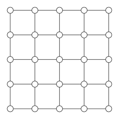
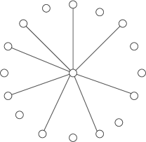
We performed experiments for three different classes of graphs: four-nearest neighbor lattices, (b) eight-nearest neighbor lattices, and (c) star-shaped graphs, as illustrated in Figure 1.

(a)		(b)		(c)

Figure 1: Illustrations of different graph classes used in simulations. (a) Four-nearest neighbor grid ($d=4$). (b) Eight-nearest neighbor grid ($d=8$). (c) Star-shaped graph ($d=\Theta(p)$, or $d=\Theta(\log(p))$).

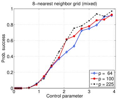
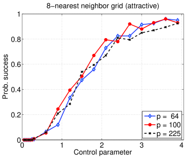
Given a distribution $\mathbb{P}_{{{\theta^{*}}}}$ of the Ising form (1), we generated random data sets $\{x^{(1)},\ldots,x^{(n)}\}$ by Gibbs sampling for the lattice models, and by exact sampling for the star graph. For a given graph class and edge strength $\omega>0$, we examined the performance of models with mixed couplings, meaning $\theta^{*}_{st}=\pm\omega$ with equal probability, or with positive couplings, meaning that $\theta^{*}_{st}=\omega$ for all edges $(s,t)$. In all cases, we set the regularization parameter as $\lambda_{n}=\Theta(\sqrt{\frac{\log p}{n}})$. Above the threshold sample size $n$ predicted by Theorem 1, this choice ensured correct model selection with high probability, consistent with the theoretical prediction. For any given graph and coupling type, we performed simulations for sample sizes $n$ scaling as $n=10\beta d\log(p)$, where the control parameter $\beta$ ranged from $0.1$ to upwards of $2$, depending on the graph type.

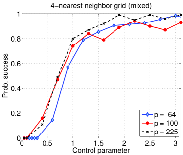
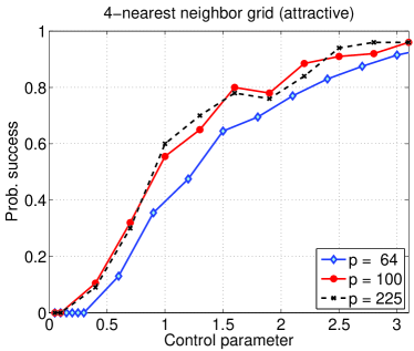
Figure 2 shows results for the $4$-nearest-neighbor grid model, illustrated in Figure 1(a), for three different graph sizes $p\in\{64,100,225\}$, with mixed couplings (panel (a)) and attractive couplings (panel (b)). Each curve corresponds to a given problem size, and corresponds to the success probability versus the control parameter $\beta$. Each point corresponds to the average of $N=200$ trials. Notice how despite the very different regimes of $(n,p)$ that underlie each curve, the different curves all line up with one another quite well. This fact shows that for a fixed degree graph (in this case $\deg=4$), the ratio $n/\log(p)$ controls the success/failure of our model selection procedure, consistent with the prediction of Theorem 1.

(a)	(b)

Figure 2: Plots of success probability $\mathbb{P}[\widehat{\mathcal{N}}_{\pm}(r)=\mathcal{N}(r),\forall r]$ versus the control parameter $\beta(n,p,d)=n/[10d\log(p)]$ for Ising models on 2-D grids with four nearest-neighbor interactions ($d=4$). (a) Randomly chosen mixed sign couplings $\theta^{*}_{st}=\pm 0.50$. (b) All positive couplings $\theta^{*}_{st}=0.50$.

Figure 3 shows analogous results for the $8$-nearest-neighbor lattice model ($d=8$), for the same range of problem size $p\in\{64,100,225\}$, as well as both mixed and attractive couplings. Notice how once again the curves for different problem sizes are all well-aligned, consistent with the prediction of Theorem 1.

(a)	(b)

Figure 3: Plots of success probability $\mathbb{P}[\widehat{\mathcal{N}}_{\pm}(r)=\mathcal{N}(r),\forall r]$ versus the control parameter $\beta(n,p,d)=n/[10d\log(p)]$ for Ising models on 2-D grids with eight nearest-neighbor interactions ($d=8$). (a) Randomly chosen mixed sign couplings $\theta^{*}_{st}=\pm 0.25$. (b) All positive couplings $\theta^{*}_{st}=0.25$.

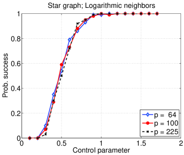
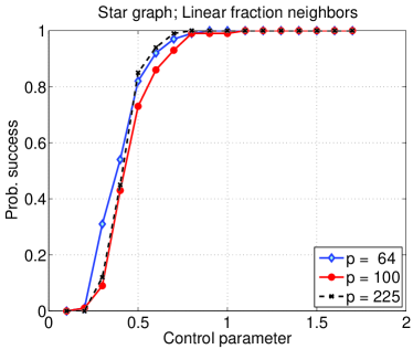
For our last set of experiments, we investigated the performance of our method for a class of graphs with unbounded maximum degree $d$. In particular, we constructed star-shaped graphs with $p$ vertices by designating one node as the spoke, and connecting it to $d<(p-1)$ of its neighbors. For linear sparsity, we chose $d=\lceil 0.1p\rceil$, whereas for logarithmic sparsity we choose $d=\lceil\log(p)\rceil$. We again studied a triple of graph sizes $p\in\{64,100,225\}$ and Figure 4 shows the resulting curves of success probability versus control parameter $\beta=n/[10d\log(p)]$. Panels (a) and (b) correspond respectively to the cases of logarithmic and linear degrees. As with the bounded degree models in Figure 2 and 3, these curves align with one another, showing a transition from failure to success with probability one.

(a)	(b)

Figure 4: Plots of success probability $\mathbb{P}[\widehat{\mathcal{N}}_{\pm}(r)=\mathcal{N}(r),\forall r]$ versus the control parameter $\beta(n,p,d)=n/[10d\log(p)]$ for star-shaped graphs, in which $d=\Theta(p)$, for attractive couplings. (a) Logarithmic growth in degrees. (b) Linear growth in degrees.

7 Conclusion

We have shown that a technique based on $\ell_{1}$-regularized logistic regression can be used to perform consistent model selection in discrete graphical models, with polynomial computational complexity and sample complexity logarithmic in the graph size. Our analysis applies to the high-dimensional setting, in which both the number of nodes $p$ and maximum neighborhood sizes $d$ are allowed to grow as a function of the number of observations $n$. There are a number of possible directions for future work. For bounded degree graphs, our results show that the structure can be recovered with high probability once $n/\log(p)$ is sufficiently large. Up to constant factors, this result matches known information-theoretic lower bounds (Bresler et al., 2008, Santhanam and Wainwright, 2008). On the other hand, our experimental results on graphs with growing degrees (star-shaped graphs) are consistent with the conjecture that the logistic regression procedure exhibits a threshold at a sample size $n=\Theta(d\log p)$, at least for problems where the minimum value $\theta^{*}_{\operatorname{min}}$ stays bounded away from zero. It would be interesting to provide a sharp threshold result for this problem, to parallel the known thresholds for $\ell_{1}$-regularized linear regression, or the Lasso (see Wainwright (2006)). Finally, the ideas described here, while specialized in this paper to the pairwise binary case, are more broadly applicable to discrete graphical models with a higher number of states; this is an interesting direction for future research.

Acknowledgements

Research supported in part by NSF grants IIS-0427206 and CCF-0625879 (PR and JL), NSF grants DMS-0605165 and CCF-0545862 (PR and MJW), and a Siebel Scholarship (PR).

Appendix A Proofs for Section 4.1

In this section, we provide proofs of Lemmas 2, Lemma 3 and Lemma 4, previously stated in Section 4.1.

A.1 Proof of Lemma 2

Note that any entry of $W^{n}$ has the form $W^{n}_{u}=\frac{1}{n}\sum_{i=1}^{n}Z^{(i)}_{u}$, where for $i=1,2,\ldots,n$, the variables

$$Z^{(i)}_{u} := x^{(i)}_{\backslash r}\left\{x^{(i)}_{r}-\mathbb{P}_{{{\theta^{*}}}}[x_{r}=1\,\mid\,x^{(i)}_{\backslash r}]+\mathbb{P}_{{{\theta^{*}}}}[x_{r}=-1\,\mid\,x^{(i)}_{\backslash r}]\right\}$$

are zero-mean under $\mathbb{P}_{{{\theta^{*}}}}$, i.i.d., and bounded ($|Z^{(i)}_{u}|\leq 2$). Therefore, by the Azuma-Hoeffding inequality (Hoeffding, 1963), we have, for any $\delta>0$, $\mathbb{P}\left[|W^{n}_{u}|>\delta\right]\leq 2\exp\left(-\frac{n\delta^{2}}{8}\right)$. Setting $\delta=\frac{\alpha_{\operatorname{{\scriptstyle{}}}}\lambda_{n}}{4\,(2-\alpha_{\operatorname{{\scriptstyle{}}}})}$, we obtain

$$\mathbb{P}\left[\frac{2-\alpha_{\operatorname{{\scriptstyle{}}}}}{\lambda_{n}}|W^{n}_{u}|>\frac{\alpha_{\operatorname{{\scriptstyle{}}}}}{4}\right] \leq 2\exp\left(-Kn\lambda^{2}_{n}\right)$$

for some constant $K$. Finally, applying a union bound over the indices $u$ of $W^{n}$ yields

$$\mathbb{P}\left[\frac{2-\alpha_{\operatorname{{\scriptstyle{}}}}}{\lambda_{n}}\|W^{n}\|_{\infty}>\frac{\alpha_{\operatorname{{\scriptstyle{}}}}}{4}\right] \leq 2\exp\left(-Kn\lambda^{2}_{n}+\log(p)\right),$$

as claimed.

A.2 Proof of Lemma 3

Following a method of Rothman et al. (2008), we define the function $G:{\mathbb{R}}^{d}\rightarrow{\mathbb{R}}$ by

$$G(u_{S}) :\,=\ell(\theta^{*}_{S}+u_{S};\{x^{(i)}\})-\ell(\theta^{*}_{S};\{x^{(i)}\})+\lambda_{n}\left(\|\theta^{*}_{S}+u_{S}\|-\|\theta^{*}_{S}\|\right).$$ (50)

It can be seen from equation (24) that $\widehat{u}=\widehat{\theta}_{S}-\theta^{*}_{S}$ minimizes $G$. Moreover $G(0)=0$ by construction; therefore, we must have $G(\widehat{u})\leq 0$. Note also that $G$ is convex. Suppose that we show that for some radius $B>0$, and for $u\in{\mathbb{R}}^{d}$ with $\|u\|_{2}=B$, we have $G(u)>0$. We then claim that $\|\widehat{u}\|_{2}\leq B$. Indeed, if $\widehat{u}$ lay outside the ball of radius $B$, then the convex combination $t\widehat{u}+(1-t)(0)$ would lie on the boundary of the ball, for an appropriately chosen $t\in(0,1)$. By convexity,

$$G\left(t\widehat{u}+(1-t)(0)\right)\;\leq\;tG(\widehat{u})+(1-t)G(0)\,\leq\,0,$$

contradicting the assumed strict positivity of $G$ on the boundary.

It thus suffices to establish strict positivity of $G$ on the boundary of the ball with radius $B=M\lambda_{n}\sqrt{d}$, where $M>0$ is a parameter to be chosen later in the proof. Let $u\in{\mathbb{R}}^{d}$ be an arbitrary vector with $\|u\|_{2}=B$. Recalling the notation $W=\nabla\ell({{\theta^{*}}};\{x^{(i)}\})$, by a Taylor series expansion of the log likelihood component of $G$, we have

$$G(u) = W_{S}^{T}u+u^{T}\left[\nabla^{2}\ell(\theta^{*}_{S}+\alpha u)\right]u+\lambda_{n}\left(\|\theta^{*}_{S}+u_{S}\|-\|\theta^{*}_{S}\|\right),$$ (51)

for some $\alpha\in[0,1]$. For the first term, we have the bound

$$|W_{S}^{T}u| \leq \|W_{S}\|_{\infty}\|u\|_{1}\;\leq\;\|W_{S}\|_{\infty}\sqrt{d}\,\|u\|_{2}\;\leq\;\left(\lambda_{n}\sqrt{d}\right)^{2}\frac{M}{4},$$ (52)

since $\|W_{S}\|_{\infty}\leq\frac{\lambda_{n}}{4}$ with probability converging to one from Lemma 2.

Applying the triangle inequality to the last term in the expansion (51) yields

$$\lambda_{n}\|\theta^{*}_{S}+u_{S}\|_{1}-\|\theta^{*}_{S}\|_{1} \geq-\lambda_{n}\|u_{S}\|_{1}\,\geq\;-\lambda_{n}\sqrt{d}\|u_{S}\|_{2}\;=\;-M\left(\sqrt{d}\lambda_{n}\right)^{2}.$$ (53)

Finally, turning to the middle Hessian term, we have

$$q^{*} :=\;\Lambda_{min}(\nabla^{2}\ell(\theta^{*}_{S}+\alpha u;\{x^{(i)}\}))$$

$$\geq\;\min_{\alpha\in[0,1]}\Lambda_{min}(\nabla^{2}\ell(\theta^{*}_{S}+\alpha u_{S};\{x^{(i)}\}))$$

$$=\;\min_{\alpha\in[0,1]}\Lambda_{min}\left[\frac{1}{n}\sum_{i=1}^{n}\eta(x^{(i)};\theta^{*}_{S}+\alpha u_{S})x^{(i)}_{S}(x^{(i)}_{S})^{T}\right]$$

By a Taylor series expansion of $\eta(x^{(i)};\cdot)$, we have

$$q^{*} \geq\;\Lambda_{min}\left[\frac{1}{n}\sum_{i=1}^{n}\eta(x^{(i)};\theta^{*}_{S})x^{(i)}_{S}(x^{(i)}_{S})^{T}\right]$$

$$\qquad\quad-\max_{\alpha\in[0,1]}|\!|\!|\frac{1}{n}\sum_{i=1}^{n}\eta^{\prime}(x^{(i)};\theta^{*}_{S}+\alpha u_{S})(u_{S}^{T}x^{(i)}_{S})x^{(i)}_{S}(x^{(i)}_{S})^{T}|\!|\!|_{{2}}$$

$$=\;\Lambda_{min}(Q^{*}_{SS})-\max_{\alpha\in[0,1]}|\!|\!|\frac{1}{n}\sum_{i=1}^{n}\eta^{\prime}(x^{(i)};\theta^{*}_{S}+\alpha u_{S})(u_{S}^{T}x^{(i)}_{S})x^{(i)}_{S}(x^{(i)}_{S})^{T}|\!|\!|_{{2}}$$

$$\geq C_{min}-\max_{\alpha\in[0,1]}|\!|\!|\frac{1}{n}\sum_{i=1}^{n}\eta^{\prime}(x^{(i)};\theta^{*}_{S}+\alpha u_{S})(u_{S}^{T}x^{(i)}_{S})x^{(i)}_{S}(x^{(i)}_{S})^{T}|\!|\!|_{{2}}$$

It remains to control the final spectral norm. For any fixed $\alpha\in[0,1]$ and $y\in{\mathbb{R}}^{d}$ with $\|y\|_{2}=1$, we have

$$y^{T}\left\{\frac{1}{n}\sum_{i=1}^{n}\eta^{\prime}(x^{(i)};\theta^{*}_{S}+\alpha u_{S})(u_{S}^{T}x^{(i)}_{S})x^{(i)}_{S}(x^{(i)}_{S})^{T}\right\}y\;=\;$$

$$\frac{1}{n}\sum_{i=1}^{n}\eta^{\prime}(x^{(i)};\theta^{*}_{S}+\alpha u_{S})(u_{S}^{T}x^{(i)}_{S})\;\left[x^{(i)}_{S})^{T}y\right]^{2}$$

$$\leq \frac{1}{n}\sum_{i=1}^{n}\left|\eta^{\prime}(x^{(i)};\theta^{*}_{S}+\alpha u_{S})(u_{S}^{T}x^{(i)}_{S})\right|\;\left[x^{(i)}_{S})^{T}y\right]^{2}$$

Now note that $|\eta^{\prime}(x^{(i)};\theta^{*}_{S}+\alpha u_{S})|\leq 1$, and $|u_{S}^{T}x^{(i)}_{S}|\leq\sqrt{d}\|u_{S}\|_{2}=M\lambda_{n}d$. Moreover, we have $\|\frac{1}{n}\sum_{i=1}^{n}\left(x^{(i)}_{S})^{T}y\right)\leq\|\frac{1}{n}\sum_{i=1}^{n}x^{(i)}_{S}(x^{(i)}_{S})^{T}\|_{2}\;\leq\;D_{\operatorname{max}}$ by assumption. Combining these pieces, we obtain

$$\max_{\alpha\in[0,1]}|\!|\!|\frac{1}{n}\sum_{i=1}^{n}\eta^{\prime}(x^{(i)};\theta^{*}_{S}+\alpha u_{S})(u_{S}^{T}x^{(i)}_{S})x^{(i)}_{S}(x^{(i)}_{S})^{T}|\!|\!|_{{2}} \leq D_{\operatorname{max}}M\lambda_{n}d$$

$$\leq \frac{C_{min}}{2},$$

where the last inequality follows as long as $\lambda_{n}d\leq\frac{C_{min}}{2D_{\operatorname{max}}M}$. We have thus shown that

$$q^{*}:=\Lambda_{min}(\nabla^{2}\ell(\theta^{*}_{S}+\alpha u;\{x^{(i)}\})) \geq \frac{C_{min}}{2}$$ (54)

with probability converging to one, as long as $\lambda_{n}d$ is sufficiently small.

Finally, combining the bounds (52),  (53), and (54) in the expression (51), we conclude that

$$G(u_{S}) \geq \left(\lambda_{n}\sqrt{d}\right)^{2}\,\left\{-\frac{1}{4}M+\frac{C_{min}}{2}M^{2}-M\right\}.$$

This expression is strictly positive for $M=5/C_{min}$. Moreover, for this choice of $M$, we have that $\lambda_{n}d$ must be upper bounded by $\frac{C_{min}}{2D_{\operatorname{max}}M}=\frac{C_{min}^{2}}{10D_{\operatorname{max}}}$, as assumed in the lemma statement.

A.3 Proof of Lemma 4

We first show that the remainder term $R^{n}$ satisfies the bound $\|R^{n}\|_{\infty}\leq D_{\operatorname{max}}\|\widehat{\theta}_{S}-\theta^{*}_{S}\|_{2}^{2}$. Then the result of Lemma 3—namely, that $\|\widehat{\theta}_{S}-\theta^{*}_{S}\|_{2}=\mathcal{O}_{p}(\lambda_{n}\sqrt{d})$—can be used to conclude that
$\frac{\|R^{n}\|_{\infty}}{\lambda_{n}}=\mathcal{O}_{p}(\lambda_{n}d)$, which suffices to guarantee the claim of Lemma 4.

Focusing on element $R^{n}_{j}$ for some index $j\in\{1,\ldots,p\}$, we have

$$R^{n}_{j} = \left[\nabla^{2}\ell(\bar{\theta}^{(j)};x)-\nabla^{2}\ell({{\theta^{*}}};x)\right]_{j}^{T}\,[\widehat{\theta}-\theta^{*}]$$

$$= \frac{1}{n}\sum_{i=1}^{n}\left[\eta(x^{(i)};\bar{\theta}^{(j)})-\eta(x^{(i)};{{\theta^{*}}})\right]\left[x^{(i)}(x^{(i)})^{T}\right]_{j}^{T}[\widehat{\theta}-\theta^{*}].$$

for some point $\bar{\theta}^{(j)}=t_{j}\widehat{\theta}+(1-t_{j}){{\theta^{*}}}$. Setting $g(t)=\frac{4\exp(2t)}{[1+\exp(2t)]^{2}}$, note that $\eta(x;\theta)=g(x_{r}\sum_{t\in V\backslash r}\theta_{rt}x_{t})$. By the chain rule and another application of the mean value theorem, we then have

$$R^{n}_{j} = \frac{1}{n}\sum_{i=1}^{n}g^{\prime}\left(\bar{\bar{\theta}}^{(j)T}x^{(i)}\right)(x^{(i)})^{T}[\bar{\theta}^{(j)}-\theta^{*}]\left\{x^{(i)}_{j}(x^{(i)})^{T}[\widehat{\theta}-\theta^{*}]\right\}$$

$$= \frac{1}{n}\sum_{i=1}^{n}\left\{g^{\prime}\left(\bar{\bar{\theta}}^{(j)T}x^{(i)}\right)x^{(i)}_{j}\right\}\left\{\bar{\theta}^{(j)}-{{\theta^{*}}}]^{T}x^{(i)}(x^{(i)})^{T}[\widehat{\theta}-\theta^{*}]\right\}$$

where $\bar{\bar{\theta}}^{(j)}$ is another point on the line joining $\widehat{\theta}$ and ${{\theta^{*}}}$. Setting $a_{i}:=\{g^{\prime}\left(\bar{\bar{\theta}}^{(j)T}x^{(i)}\right)x^{(i)}_{j}\}$ and $b_{i}:=\{[\bar{\theta}^{(j)}-\theta^{*}]^{T}x^{(i)}(x^{(i)})^{T}[\widehat{\theta}-\theta^{*}]\}$, we have

$$|R^{n}_{j}| = \frac{1}{n}\left|\sum_{i=1}^{n}a_{i}b_{i}\right|\;\leq\;\frac{1}{n}\|a\|_{\infty}\|b\|_{1}.$$

A calculation shows that $\|a\|_{\infty}\leq 1$, and

$$\frac{1}{n}\|b\|_{1} = t_{j}[\widehat{\theta}-\theta^{*}]^{T}\left\{\frac{1}{n}\sum_{i=1}^{n}x^{(i)}(x^{(i)})^{T}\right\}[\widehat{\theta}-\theta^{*}]$$

$$= t_{j}[\widehat{\theta}_{S}-\theta^{*}_{S}]^{T}\left\{\frac{1}{n}\sum_{i=1}^{n}x^{(i)}_{S}(x^{(i)}_{S})^{T}\right\}[\widehat{\theta}_{S}-\theta^{*}_{S}]$$

$$\leq D_{\operatorname{max}}\|\widehat{\theta}_{S}-\theta^{*}_{S}\|_{2}^{2},$$

where the second line uses the fact that $\widehat{\theta}_{S^{c}}=\theta^{*}_{S^{c}}=0$. This concludes the proof.

Appendix B Proof of Lemma 7

Recall from the discussion leading up to the bound (43) that element $(j,k)$ of the matrix difference $Q^{n}-Q^{*}$, denoted by $Z_{jk}$, satisfies a sharp tail bound. By definition of the $\ell_{\infty}$-matrix norm, we have

$$\mathbb{P}[|\!|\!|Q^{n}_{{S^{c}}S}-Q^{*}_{{S^{c}}S}|\!|\!|_{{\infty}}\geq\delta] = \mathbb{P}[\max_{j\in{S^{c}}}\sum_{k\in S}|Z_{jk}|\geq\delta]$$

$$\leq (p-d)\,\mathbb{P}[\sum_{k\in S}|Z_{jk}|\geq\delta],$$

where the final inequality uses a union bound, and the fact that $|{S^{c}}|\leq p-d$. Via another union bound over the row elements, we have

$$\mathbb{P}[|\!|\!|Q^{n}_{{S^{c}}S}-Q^{*}_{{S^{c}}S}|\!|\!|_{{\infty}}\geq\delta] \leq(p-d)\;d\;\mathbb{P}\left[|Z_{jk}|\geq\delta/d\right],$$

from which the claim (46a) follows by setting $\epsilon=\delta/d$ in the Hoeffding bound (43). The proof of bound (46b) is analogous, with the pre-factor $(p-d)$ replaced by $d$.

To prove the last claim (46c), we write

$$|\!|\!|(Q^{n}_{SS})^{-1}-(Q^{*}_{SS})^{-1}|\!|\!|_{{\infty}} = |\!|\!|(Q^{*}_{SS})^{-1}\left[Q^{*}_{SS}-Q^{n}_{SS}\right](Q^{n}_{SS})^{-1}|\!|\!|_{{\infty}}$$

$$\leq \sqrt{d}\;|\!|\!|(Q^{*}_{SS})^{-1}\left[Q^{*}_{SS}-Q^{n}_{SS}\right](Q^{n}_{SS})^{-1}|\!|\!|_{{2}}$$

$$\leq \sqrt{d}\;|\!|\!|(Q^{*}_{SS})^{-1}|\!|\!|_{{2}}|\!|\!|Q^{*}_{SS}-Q^{n}_{SS}|\!|\!|_{{2}}|\!|\!|(Q^{n}_{SS})^{-1}|\!|\!|_{{2}}$$

$$\leq \frac{\sqrt{d}}{C_{min}}|\!|\!|Q^{*}_{SS}-Q^{n}_{SS}|\!|\!|_{{2}}|\!|\!|(Q^{n}_{SS})^{-1}|\!|\!|_{{2}}.$$

From the proof of Lemma 5, in particular equation (44), we have

$$\mathbb{P}\left[|\!|\!|(Q^{n}_{SS})^{-1}|\!|\!|_{{2}}\geq\frac{2}{C_{min}}\right] \leq 2\exp\left(-K\frac{\delta^{2}n}{d^{2}}+B\log(d)\right)$$

for a constants $B$. Moreover, from equation (44), we have

$$\mathbb{P}[|\!|\!|Q^{n}_{SS}-Q_{SS}|\!|\!|_{{2}}\geq\delta/\sqrt{d}] \leq 2\exp\left(-K\frac{\delta^{2}n}{d^{3}}+2\log(d)\right),$$

so that the bound (46c) follows.

References

- Abbeel et al. (2006) P. Abbeel, D. Koller, and A. Y. Ng. Learning factor graphs in polynomial time and sample complexity. Jour. Mach. Learning Res., 7:1743–1788, 2006.
- Bertsekas (1995) D.P. Bertsekas. Nonlinear programming. Athena Scientific, Belmont, MA, 1995.
- Bresler et al. (2008) G. Bresler, E. Mossel, and A. Sly. Reconstruction of Markov random fields from samples: Some easy observations and algorithms. http://front.math.ucdavis.edu/0712.1402, 2008.
- Candes and Tao (2006) E. Candes and T. Tao. The Dantzig selector: Statistical estimation when is much larger than . Annals of Statistics, 2006.
- Chickering (1995) D. Chickering. Learning Bayesian networks is NP-complete. Proceedings of AI and Statistics, 1995.
- Chow and Liu (1968) C. Chow and C. Liu. Approximating discrete probability distributions with dependence trees. IEEE Trans. Info. Theory, 14(3):462–467, 1968.
- Csiszár and Talata (2006) I. Csiszár and Z. Talata. Consistent estimation of the basic neighborhood structure of Markov random fields. The Annals of Statistics, 34(1):123–145, 2006.
- Dasgupta (1999) S. Dasgupta. Learning polytrees. In Uncertainty on Artificial Intelligence, pages 134–14, 1999.
- Davidson and Szarek (2001) K. R. Davidson and S. J. Szarek. Local operator theory, random matrices, and Banach spaces. In Handbook of Banach Spaces, volume 1, pages 317–336. Elsevier, Amsterdan, NL, 2001.
- Donoho and Elad (2003) D. Donoho and M. Elad. Maximal sparsity representation via minimization. Proc. Natl. Acad. Sci., 100:2197–2202, March 2003.
- Hoeffding (1963) W. Hoeffding. Probability inequalities for sums of bounded random variables. Journal of the American Statistical Association, 58:13–30, 1963.
- Horn and Johnson (1985) R. A. Horn and C. R. Johnson. Matrix Analysis. Cambridge University Press, Cambridge, 1985.
- Koh et al. (2007) K. Koh, S. J. Kim, and S. Boyd. An interior-point method for large-scale -regularized logistic regression. Jour. Mach. Learning Res., 3:1519–1555, 2007.
- Meinshausen and Bühlmann (2006) N. Meinshausen and P. Bühlmann. High dimensional graphs and variable selection with the lasso. Annals of Statistics, 34(3), 2006.
- Ng (2004) A. Y. Ng. Feature selection, vs. regularization, and rotational invariance. In International Conference on Machine Learning, 2004.
- Rockafellar (1970) G. Rockafellar. Convex Analysis. Princeton University Press, Princeton, 1970.
- Rothman et al. (2008) A. Rothman, P. Bickel, E. Levina, and J. Zhu. Sparse permutation invariant covariance estimation. Electronic Journal on Statistics, 2008. To appear.
- Santhanam and Wainwright (2008) N. P. Santhanam and M. J. Wainwright. Information-theoretic limits of high-dimensional model selection. In International Symposium on Information Theory, Toronto, Canada, July 2008.
- Spirtes et al. (2000) P. Spirtes, C. Glymour, and R. Scheines. Causation, prediction and search. MIT Press, 2000.
- Srebro (2003) N. Srebro. Maximum likelihood bounded tree-width Markov networks. Artificial Intelligence, 143(1):123–138, 2003.
- Tropp (2006) J. A. Tropp. Just relax: Convex programming methods for identifying sparse signals. IEEE Trans. Info. Theory, 51(3):1030–1051, March 2006.
- Wainwright (2006) M. J. Wainwright. Sharp thresholds for high-dimensional and noisy sparsity recovery using -constrained quadratic programs. In Proc. Allerton Conference on Communication, Control and Computing, October 2006. Long version: UC Berkeley Technical Report 709, May 2006.
- Wainwright et al. (2007) M. J. Wainwright, P. Ravikumar, and J. D. Lafferty. High-dimensional graphical model selection using -regularized logistic regression. In B. Schölkopf, J. Platt, and T. Hoffman, editors, Advances in Neural Information Processing Systems 19, pages 1465–1472. MIT Press, Cambridge, MA, 2007.
- Zhao and Yu (2007) P. Zhao and B. Yu. On model selection consistency of lasso. J. of Mach. Learn. Res., 7:2541–2567, 2007.