Search for a stochastic gravitational-wave signal in the second round of the Mock LISA Data Challenges

Abstract

The analysis method currently proposed to search for isotropic stochastic radiation of primordial or astrophysical origin with the Laser Interferometer Space Antenna (LISA) relies on the combined use of two LISA channels, one of which is insensitive to gravitational waves, such as the symmetrised Sagnac. For this method to work, it is essential to know how the instrumental noise power in the two channels are related to one another; however, no quantitative estimates of this key information are available to date. The purpose of our study is to assess the performance of the symmetrised Sagnac method for different levels of prior information regarding the instrumental noise. We develop a general approach in the framework of Bayesian inference and an end-to-end analysis algorithm based on Markov Chain Monte Carlo methods to compute the posterior probability density functions of the relevant model parameters. We apply this method to data released as part of the second round of the Mock LISA Data Challenges. For the selected (and somewhat idealised) cases considered here, we find that a prior uncertainty of a factor $\approx 2$ in the ratio between the power of the instrumental noise contributions in the two channels allows for the detection of isotropic stochastic radiation. More importantly, we provide a framework for more realistic studies of LISA’s performance and development of analysis techniques in the context of searches for stochastic signals.

, ,

1 Introduction

The Laser Interferometer Space Antenna (LISA) [1] will observe many different gravitational-wave signals, including stochastic gravitational radiation from a variety of sources. The gravitational-wave foreground produced by galactic white dwarf binaries is a guaranteed (anisotropic) signal [2, 3, 4, 5, 6], but one also expects LISA to see other types of stochastic gravitational radiation, possibly including (isotropic) backgrounds from the very early universe [7, 8, 9, 10] and foregrounds from populations of extra-galactic sources [11, 12]. For anisotropic foregrounds, the stochastic signal will be modulated, with a period of one year, by LISA’s orbital motion around the Sun. Hence search techniques that take advantage of this modulation can be used to distinguish the astrophysical signal from instrumental noise [13, 14, 15, 16, 17, 18, 6]. For isotropic backgrounds, an alternative search method is needed, which will work in the absence of any (statistical) time-variation of the signal relative to the noise.

One approach that has been proposed to search for isotropic gravitational radiation is to use a particular combination of the LISA output, called the symmetrised Sagnac channel [19], as a real-time noise monitor for LISA. This is possible at low-frequencies (i.e., less than a few mHz), since the response of the symmetrised Sagnac channel to gravitational waves is highly suppressed for these frequencies. One can then compare the power in the symmetrised Sagnac channel to that in another observable that is sensitive to gravitational waves, and then ‘subtract’ the two to estimate the power in the gravitational-wave background [19, 20]. For this subtraction method to work, one needs to know how the instrumental noise power in the two channels are related to one another. Otherwise, one might falsely assign too much (little) power to the gravitational-wave component if one underestimates (overestimates) the instrumental noise power in the gravitational-wave channel. Obviously, one cannot unambiguously observe isotropic stochastic radiation without any prior knowledge about the instrumental noise.

In this paper, we extend the analyses of [19, 20] by recasting the symmetrised Sagnac method in the framework of Bayesian inference; we then use it to search for stochastic gravitational-wave signals in data taken from round 2 of the Mock LISA Data Challenge (MLDC) [21, 22, 23, 24]. (These are mock data sets released by the MLDC Taskforce, which contain simulated data from simplified models of LISA and restricted numbers of astrophysical sources.) The purpose of our study is to assess the performance of the symmetrised Sagnac method for different levels of prior information regarding the instrumental noise. Using Markov Chain Monte Carlo (MCMC) methods to calculate the posterior probability density functions (PDFs) of the relevant parameters, we explicitly show how the uncertainty in our estimate of the gravitational-wave signal power depends on our prior knowledge of the relationship between the instrumental noise power in the symmetrised Sagnac and gravitational-wave channels. In particular, we find that a prior uncertainty of a factor $\approx 2$ in the ratio between the power of the instrumental noise contributions in the two channels allows for the detection of isotropic stochastic radiation. For the specific case considered here (and driven by the MLDC data sets released in Challenge 2), in which the amplitude of the gravitational-wave signal dominates the instrumental noise, a more accurate knowledge of this ratio, say within a factor of $\approx 10\%$, provides only a marginal improvement for signal detection. This particular result depends of course on the signal-to-noise ratio, and we do not try, in this paper, to answer conclusively this question of detectability as a function of signal-to-noise ratio and prior information. Nonetheless, we provide a conceptually transparent framework that allows us to quantitatively investigate this problem; the formalism enables more realistic studies of LISA’s performance and associated requirements in the context of searches for stochastic signals that could yield some of the most exiting discoveries of the mission. Some of these issues are currently under investigation and will be discussed in detail in a forthcoming paper [25].

The rest of the paper is organised as follows: In Sec. 2, we present details of the analysis method, and its application to LISA. In Sec. 3, we give the results of our analysis when applied to the MLDC data sets. Finally, in Sec. 4 we summarise our findings and discuss possible extensions for future investigations.

2 Analysis method

2.1 LISA time-delay interferometry combinations $A$, $E$, and $T$

LISA will consist of three spacecraft in a (nearly) equilateral configuration of side $5\times 10^{6}$ km, trailing the Earth by about 20 degrees. The distances between the spacecraft will be modulated by incident gravitational waves at the level of picometres. The modulation will be sensed by monitoring the frequency (or, equivalently, phase) of laser beams exchanged between the spacecraft, and comparing this to locally-generated reference laser signals.

The six raw Doppler measurements can be combined in various ways using the principle of Time-Delay Interferometry (TDI) [26]. We use the first-generation TDI combinations, in which it is assumed that LISA is rigid and symmetric, and that laser frequency noise cancels completely. This is consistent with the conventions adopted in the context of the MLDCs [22, 28, 23, 24, 27], but the analysis presented here can be generalised to second-generation TDI. In particular, we work with the $A$, $E$ and $T$ combinations, which are independent and noise-orthogonal [29]. For frequencies smaller than the inverse of the light travel-time down a LISA arm ($1/16.6\ {\rm s}\simeq 10\ {\rm mHz}$), the $A$ and $E$ combinations are equivalent to two unequal-arm Michelson interferometers, with independent noise, rotated at 45 degrees to each other, and thus are sensitive to the two orthogonal polarisations of gravitational waves. For these low frequencies, the response of the $T$ channel to gravitational-waves is highly-suppressed (similar to the response of the standard symmetrised Sagnac combination $\zeta$), and hence can be used as a real-time noise monitor, as discussed above. For simplicity, in what follows, we will restrict attention to the $A$ and $T$ channels. The analysis can easily be extended to also include $E$, which will improve our ability to detect gravitational waves by reducing the uncertainty in our estimates by a factor of $\sqrt{2}$ [25].

2.2 Bayesian inference

For low frequencies, the output of the $A$ and $T$ channels in the frequency domain have the form

$$\tilde{A}=\tilde{n}_{A}+\tilde{h}\,,\qquad\tilde{T}=\tilde{n}_{T}\,,$$ (1)

where $\tilde{n}_{A,T}$ denote the instrumental noise in the two channels, and $\tilde{h}$ denotes the stochastic gravitational-wave signal. (Here $\widetilde{\ }$ denotes the discrete Fourier transform of the time domain data, so that $\tilde{A}$, $\tilde{T}$, etc. are dimensionless quantities.) Notice that we assume that in the frequency window of interest the gravitational-wave contribution is perfectly suppressed in the $T$ channel. We also assume that the instrumental noises and stochastic signal are zero-mean Gaussian random variables, with variances

$$\langle|\tilde{n}_{A}|^{2}\rangle=\sigma_{A}^{2}\,,\qquad\langle|\tilde{n}_{T}|^{2}\rangle=\sigma_{T}^{2}\,,\qquad\langle|\tilde{h}|^{2}\rangle=\sigma_{h}^{2}\,,$$ (2)

and that the noises in the two channels are related by

$$\sigma_{A}^{2}=a\sigma_{T}^{2}\,,$$ (3)

where $a$ is some multiplicative factor, which we may not know in advance. (The variances $\sigma_{A}^{2}$, $\sigma_{T}^{2}$, $\sigma_{h}^{2}$, and multiplicative factor $a$ all vary as functions of frequency; however, in the analysis below we consider one frequency bin at a time, and therefore do not explicitly show the dependence of these variables on frequency.) Since the noise in the $\tilde{A}$ and $\tilde{T}$ channels are uncorrelated with one another and with the gravitational-wave signal, the covariance matrix is

$$C=\left(\begin{array}[]{cc}a\sigma_{T}^{2}+\sigma_{h}^{2}&0\\ 0&\sigma_{T}^{2}\end{array}\right).$$ (4)

Note that the problem consists, in general, of three unknown variables, $\vec{\theta}\equiv(\sigma_{h}^{2},\sigma_{T}^{2},a)$. Measurements of the two channels $\vec{d}\equiv(\tilde{A},\tilde{T})$ give us only two independent constraints.

Application of Bayes’ theorem allows us to construct the joint posterior probability density function (PDF) of the unknown parameters

$$p(\vec{\theta}|\vec{d})=\frac{p(\vec{\theta})p(\vec{d}|\vec{\theta})}{p(\vec{d})}\,,$$ (5)

where $p(\vec{\theta})$ is the joint prior PDF of the parameters, $p(\vec{d}|\vec{\theta})$ is the likelihood function, and $p(\vec{d})$, the so-called evidence or marginal likelihood, can be regarded simply as a normalisation constant throughout. The likelihood function for a single frequency bin is a multivariate Gaussian

$$p(\vec{d}|\vec{\theta})=\frac{1}{2\pi}\frac{1}{\sqrt{\det{C}}}\exp{\left[-\frac{1}{2}\sum_{i,j=1}^{2}d_{i}^{*}[C^{-1}]_{ij}d_{j}\right]}\,,$$ (6)

where $C$ is the noise covariance matrix given by (4). We can construct a likelihood function for multiple time segments by simply multiplying the likelihoods of the individual segments.

The posterior PDF for any given parameter (or subset of parameters), say $\theta_{1}$, can be obtained by marginalising the joint posterior over the remaining parameters:

$$p(\theta_{1}|\vec{d})=\int d\theta_{2}\int d\theta_{3}\>p(\vec{\theta}|\vec{d})\,.$$ (7)

Markov Chain Monte Carlo (MCMC) methods can be used to explore the posterior PDFs, and to find the marginal posterior PDF on each parameter. From the marginal posteriors one can then compute the posterior mean on each parameter:

$$\bar{\theta}_{i}=\int_{-\infty}^{\infty}d\theta_{i}\>\theta_{i}p(\theta_{i}|\vec{d})\,,$$ (8)

and the $95\%$ probability intervals $[\theta_{i,{\rm low}},\theta_{i,{\rm high}}]$, where the limits define the smallest interval containing $95\%$ of the total probability:

$$0.95=\int_{\theta_{i,{\rm low}}}^{\theta_{i,{\rm high}}}d\theta_{i}\>p(\theta_{i}|\vec{d})\,.$$ (9)

The prior PDFs contain the information we have about the parameters before making the observations. For our analysis we assume no prior knowledge of the variances $\sigma_{h}^{2}$ and $\sigma_{T}^{2}$, and choose flat priors

$$p(\sigma_{h}^{2})\propto\left\{\begin{array}[]{ll}1&\mathrm{for\,\,\,}0<\sigma_{h}^{2}<\sigma_{h,\mathrm{max}}^{2}\\ 0&\mathrm{otherwise},\end{array}\right.$$ (10)

and similarly for $\sigma_{T}^{2}$. We also used flat priors for $a$, but in order to investigate how our prior knowledge of the multiplicative factor $a$ affected the posterior PDFs, the upper and lower limits of the priors were varied, to represent different states of prior knowledge of the relative instrumental noise levels in the two channels.

3 Mock LISA Data Challenge results

3.1 MLDC data sets

The analysis method detailed above has been applied to the second round of the MLDC [23]. The data sets supplied by the MLDC Taskforce are the $X$, $Y$, and $Z$ “unequal-arm Michelson” combinations of the six optical readouts. The $A$, $E$ and $T$ combinations which we use can be constructed in the frequency domain as linear combinations of $X$, $Y$ and $Z$.

The second round of the MLDC consists of various data sets containing different classes of signals [21, 23]. The 2.1 data set, which we were primarily interested in, contains the signal from $\approx 26$ million white dwarf binaries generated according to a Galactic population model superimposed on Gaussian-stationary instrumental noise. Although the astrophysical population produces an anisotropic stochastic signal below a few mHz, with some sources generating sufficiently strong radiation to allow their identification, we apply our method to the training 2.1 data set as a proof-of-principle demonstration of the symmetrised Sagnac approach. Since the background is anisotropic, the level of the galactic signal will vary throughout the year as LISA orbits the Sun, so our method provides an estimate of the average power of the gravitational-wave signal over the total observation time.

One important point that we addressed was how to validate the results of our analysis. The first round data set 1.1.1a [21, 22] contains just instrumental noise (with the same statistical properties and spectrum as the one used for the 2.1 data sets), with one injected binary signal at 1.06 mHz, which is outside of the frequency range of our analysis. This data set could therefore be used to estimate the noise power spectral density (PSD) of the $A$ channel in the absence of a signal, and hence determine the true value of $a$, which was needed to validate our results. Figure 1 shows the PSDs of the instrumental noise in both $A$ and $T$ channels, as well as the PSD of the noise and the galactic signal in the $A$ channel.

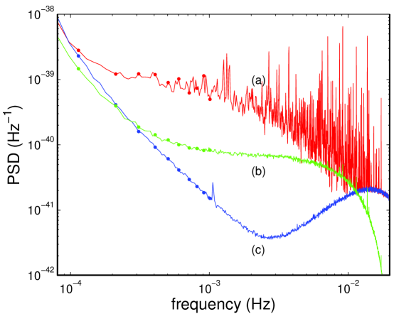
Figure 1: Power spectral densities (PSDs) obtained from the MLDC 2.1 and 1.1.1a data sets. Line (a) shows the PSD of the $A$ channel in the 2.1 data set, which includes the instrumental noise and an injected galaxy of $\approx 26$ million white dwarf binaries. Line (b) shows the PSD of the $T$ channel in the 2.1 data set. Line (c) shows the PSD of the $A$ channel in the MLDC 1.1.1a data set, which contains just one injected binary, at $1.06$ mHz, which is outside of the frequency band of interest. As there are no signals in the 1.1.1a data set below $\sim 1$ mHz, this PSD is representative of the detector noise in the $A$ channel, and was used to determine the true value of $a$, which was needed to validate the results of our analysis.

The analysis described in Sec. 2 was carried out on the first year of the 2.1 training data set. As the noises and signal are coloured (i.e., frequency-dependent) Gaussian stochastic processes, the analysis was carried-out on one frequency bin at a time. We assumed that the signal was stationary, although in reality it varies periodically over the year. The time series was split into segments of length $T_{\rm seg}=61440$s and sampling period $\Delta t=15\ {\rm s}$, which were then Fourier transformed and the bin to study was selected.

3.2 Single-bin analysis

To begin our analysis, we considered a single frequency bin centred at 0.602 mHz, and chose three different priors for $a$, see Equation (3): (i) an unconstrained prior, where $a$ ranged from 0 to $a_{\rm max}$, which was several orders of magnitude greater than the true value of $a$; (ii) a weakly-constrained prior, where $a$ ranged from 0 to twice the true value; and (iii) a strongly-constrained prior, where $a$ was known to within 10% of the true value. These three priors on $a$ correspond to no information, moderate information, and rather accurate information about the relationship between the instrumental noise levels in the $A$ and $T$ channels. For this particular analysis, the ‘true’ value of $a$ could be estimated by $P_{A}(f)/P_{T}(f)=0.43$ at 0.6 mHz, using the 1.1.1a data set, since the $A$ channel for the 1.1.1a data contains no signal in this frequency region. This allows us to assess the performance of the analysis method as a function of our a priori knowledge of the instrumental noise levels. (Of course, for a real analysis, the prior that we use for $a$ will be based largely on theoretical models of the instrument, its expected performance, and data from on-board monitoring channels that provide information on different subsystems.) The numerical values that we used for the priors are listed in Table 1.

• 	Prior on $a$ at 0.602 mHz
  ‘unconstrained’	0$<a<$	1000
  ‘weakly-constrained’	0$<a<$	0.86
  ‘strongly-constrained’	0.39$<a<$	0.47

Table 1: The three different priors on $a$ in the 0.602 mHz bin.

Figure 2 shows the resultant posterior PDFs for $\sigma_{h}^{2}$ and $\sigma_{T}^{2}$ for the three different priors distributions on $a$. It can be seen that the PDF on $\sigma_{T}^{2}$ is not dependent on the prior on $a$. This is to be expected, as $\sigma_{T}^{2}$ can be estimated from the $T$ channel alone, with no dependence on the data in the $A$ channel. The posteriors on $\sigma_{h}^{2}$ show that with no knowledge of $a$ it is impossible to determine the presence of the gravitational-wave signal. However, for this case, having moderate knowledge of $a$, even to within a factor $\approx 2$, enables us not only to distinguish the gravitational-wave signal, but also to place constraints on its value. Using the ‘strongly-constrained’ prior on $a$ does not improve the result in any appreciable manner. This is due to the fact that the stochastic signal is strong at this frequency, and in fact $\sigma_{h}/\sigma_{A}\approx 25$. The prior knowledge on $a$ required to unambiguously detect a stochastic background clearly depends on the signal-to-noise ratio; this is an important point and work is currently ongoing to address this question [25].

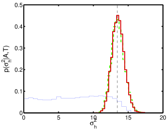
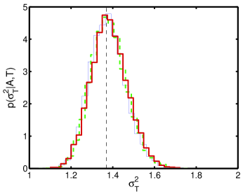
Figure 2: The marginalised posterior PDFs on (a) $\sigma_{h}^{2}$ and (b) $\sigma_{T}^{2}$ for the three different priors on $a$, using the MLDC 2.1 data. The thin line shows the posterior for the unconstrained prior on $a$, the dashed line for the weakly-constrained prior, and the thick line for the strongly-constrained prior. The vertical dashed lines indicate the expected values of the variances, obtained from the 1.1.1a and 2.1 data sets. Notice that for $\sigma_{T}^{2}$, the choice of prior on $a$ makes no difference to the posterior. For $\sigma_{h}^{2}$, no prior knowledge of $a$ means that we cannot distinguish the signal from the noise, while moderate knowledge (i.e., to within a factor of 2) enables us to easily distinguish the gravitional-wave signal and place constraints on its value.

3.3 Power spectrum estimation

In order to estimate the spectra of the gravitational-wave signal and the instrumental noise, and to gain some initial quantitative insight into the performance of the method as a function of signal-to-noise ratio, we studied nine other frequency bins distributed evenly throughout the range $0.1\ {\rm mHz}<f<1.0\ {\rm mHz}$. As before, priors on $a$ were determined using the 1.1.1a data. Strongly constrained priors, for each of these frequency bins, are given in Table 2.

• Frequency	Prior on $a$
  0.114 mHz	1.33$<a<$	1.63
  0.212 mHz	1.04$<a<$	1.27
  0.309 mHz	0.75$<a<$	0.91
  0.407 mHz	0.56$<a<$	0.68
  0.505 mHz	0.46$<a<$	0.56
  0.602 mHz	0.39$<a<$	0.47
  0.716 mHz	0.29$<a<$	0.35
  0.814 mHz	0.23$<a<$	0.29
  0.911 mHz	0.20$<a<$	0.24
  1.009 mHz	0.16$<a<$	0.20

Table 2: Strongly constrained priors on $a$ for the different frequency bins studied.

These priors were then used to calculate marginalised posterior PDFs for $\sigma_{h}^{2}$ and $\sigma_{T}^{2}$, from which the posterior mean and 95% probability interval in each band could be calculated. These values were then scaled by a factor of $2\Delta t^{2}/T_{\mathrm{seg}}$ to obtain (dimensionfull) estimates of the PSDs of the gravitational-wave signal $P_{h}(f)$ and the instrumental noise $P_{T}(f)$. Figure 3(a) shows the Bayesian 95% probability intervals for $P_{h}(f)$, and Fig. 3(b) shows the corresponding 95% probability intervals for $P_{T}(f)$.

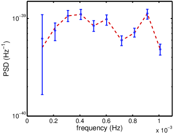
(a)

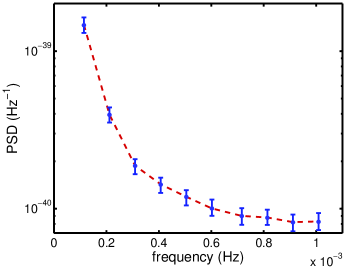
(b)

Figure 3: The estimated values of the PSDs of (a) the gravitational-wave signal, $P_{h}(f)$, and (b) the instrumental noise, $P_{T}(f)$, for ten different frequency bins. The points and error bars show the posterior means and 95% probability intervals obtained from the posterior PDFs (scaled appropriately from $\sigma_{h}^{2}$ and $\sigma_{T}^{2}$ respectively). The red dashed lines show the expected values of these PSDs as calculated from the 2.1 and 1.1.1.a data sets.

From these figures, one sees that the Bayesian estimates agree with the expected PSD estimates to within the $95\%$ probability intervals. In this band the strength of the stochastic signal $\sigma_{h}/\sigma_{A}$ varied from about 1 to $\approx 62$.

4 Conclusion

The observation of stochastic gravitational wave radiation from the early-Universe and/or astrophysical populations of sources at medium-to-high redshift may provide access to a large portion of the discovery parameter space of LISA. Because this signal is isotropic, and the standard cross-correlation technique adopted in ground-based observations [30, 31] is insensitive to such radiation due to the geometry of the LISA pseudo-Michelson observables, a new analysis approach needs to be considered. The method that has been proposed so far relies on a particular combination of the LISA output, called the symmetrised Sagnac channel [19, 20], which acts as a real-time noise monitor for LISA. To date, this approach has been put forward only at the conceptual level: it needs to be characterised quantitatively and then further developed to produce an end-to-end analysis algorithm and pipeline that can enable the science exploitation of the LISA data.

The purpose of our study was to start to assess, quantitatively, the performance of the symmetrised Sagnac method; in particular, we focused on the dependence of the method on different levels of prior information regarding the instrumental noise, and have presented here the first preliminary results of this study. We developed a general approach in the framework of Bayesian inference, and an end-to-end analysis algorithm based on Markov Chain Monte Carlo methods to compute the posterior probability density functions of the relevant model parameters. As a concrete example, we applied the method to data released as part of the second round of the Mock LISA Data Challenges [21, 22, 23, 24].

We showed that with no prior information about the ratio between the power of the instrumental noise contributions in the Sagnac and gravitational-wave-sensitive channels, it is indeed impossible to determine the presence of a stochastic gravitational-wave signal. However, for the specific cases considered here, moderate information (i.e., to within a factor $\approx 2$) about the above ratio allows one not only to determine the existence of a signal, but also to place limits on the parameters that describe it. Indeed, it is likely that the LISA instrument will be very well characterised, enabling searches for isotropic stochastic gravitational waves.

In our view the most significant outcome of our study is a framework for more realistic investigations of LISA’s performance and the development of analysis techniques in the context of searches for stochastic signals. Our approach can be immediately extended in various ways; first, by including the other independent and noise orthogonal TDI channel $E$ to improve the sensitivity of the search, and second, by parameterising the spectra in order to study the frequency dependence of the gravitational-wave signal and instrumental noises. In addition, one can investigate how the prior knowledge of the instrumental noise levels required to unambigously detect a stochastic signal depends on the signal-to-noise ratio in the gravitational-wave-sensitive channel. These extensions are currently under investigation and will be discussed in detail in a forthcoming paper [25].

References

References

- [1] Bender B L et al. 1998 LISA Pre-Phase A Report; Second Edition MPQ 233
- [2] Hils D, Bender P L and Webbink R F 1990 Astrophys. J. 360 75
- [3] Bender P L and Hils D 1997 Class. Quantum Grav. 14 1439
- [4] Hils D and Bender P L 2000 Astrophys. J. 537 334
- [5] Nelemans G, Yungelson L R and Portegies-Zwart S F 2001 Astron. Astrophys. 375 890
- [6] Edlund J A, Tinto M, Królak A and Nelemans G 2005 Phys. Rev. D 71 122003
- [7] Maggiore M 2000 Phys. Rept. 331 283
- [8] Hogan C J 2006 AIP Conf. Proc. 873 30
- [9] Damour T and Vilenkin A 2005 Phys. Rev. D 71 063510
- [10] Siemens X, Mandic V and Creighton J 2007 Phys. Rev. Lett. 98 111101
- [11] Farmer A J and Phinney E S 2003 Mon. Not. R. Astron. Soc. 346 1197
- [12] Barack L and Cutler C 2004 Phys. Rev. D 70 122002
- [13] Ungarelli C and Vecchio A 2001 Phys. Rev. D 64 121501
- [14] Cornish N J 2001 Class. Quantum Grav. 18 4277
- [15] Seto N 2004 Phys. Rev. D 69 123005
- [16] Seto N and Cooray A 2004 Phys. Rev. D 70 123005
- [17] Kudoh H and Taruya A 2005 Phys. Rev. D 71 024025
- [18] Taruya A and Kudoh H 2005 Phys. Rev. D 72 104015
- [19] Tinto M, Armstrong J W, and Estabrook F B 2000 Phys. Rev. D 63 021101(R)
- [20] Hogan C J and Bender P L 2001 Phys. Rev. D 64 062002
- [21] http://astrogravs.nasa.gov/docs/mldc/
- [22] Arnaud K A et al. (the MLDC Task Force) 2006 Laser Interferometer Space Antenna: 6th International LISA Symp. (Greenbelt, MD, 19–23 Jun 2006) ed Merkowitz S M and Livas J C (Melville, NY: AIP) 619; ibid. 625 (long version with lisaXML description: Preprint gr-qc/0609106)
- [23] Arnaud K A et al. (the MLDC Task Force) 2007 Class. Quantum Grav. 24 S551
- [24] Babak S et al. (the MLDC Task Force and Challenge 2 Participants) 2007 Proceedings of the 7th Amaldi Conference on Gravitational Waves (8–14 July 2007, Sydney, Australia) Preprint arXiv:0711.2667
- [25] Robinson E, Romano J and Vecchio A, in prep.
- [26] Tinto M and Dhurandhar S V 2005 Living Rev. Rel. 8 4
- [27] Babak S et al. (the MLDC Task Force and Challenge 1B Participants), “The Mock LISA Data Challenges: from Challenge 1B to Challenge 3” submitted to Class. Quantum Grav.
- [28] Arnaud K A et al. (the MLDC Task Force and Challenge 1 participants) 2007 Class. Quantum Grav. 24 S529
- [29] Prince T A, Tinto M, Larson S L and Armstrong J W 2002 Phys. Rev. D 66 122002
- [30] Allen B and Romano J D 1999 Phys. Rev. D 59 102001
- [31] Abbott B et al. [The LIGO Scientific Collaboration] 2007 Astrophys. J. 659 918