Design and Implementation of a Tracer Driver: Easy and Efficient Dynamic Analyses of Constraint Logic Programs

Abstract

Tracers provide users with useful information about program executions. In this article, we propose a “tracer driver”. From a single tracer, it provides a powerful front-end enabling multiple dynamic analysis tools to be easily implemented, while limiting the overhead of the trace generation. The relevant execution events are specified by flexible event patterns and a large variety of trace data can be given either systematically or “on demand”. The proposed tracer driver has been designed in the context of constraint logic programming; experiments have been made within GNU-Prolog. Execution views provided by existing tools have been easily emulated with a negligible overhead. Experimental measures show that the flexibility and power of the described architecture lead to good performance.

The tracer driver overhead is inversely proportional to the average time between two traced events. Whereas the principles of the tracer driver are independent of the traced programming language, it is best suited for high-level languages, such as constraint logic programming, where each traced execution event encompasses numerous low-level execution steps. Furthermore, constraint logic programming is especially hard to debug. The current environments do not provide all the useful dynamic analysis tools. They can significantly benefit from our tracer driver which enables dynamic analyses to be integrated at a very low cost.

To appear in Theory and Practice of Logic Programming (TPLP), Cambridge University Press.

1 Introduction

Dynamic program analysis is the process of analyzing program executions. It is generally acknowledged that dynamic analysis is complementary to static analysis; see for example the discussion of Ball [Ball (1999)]. Dynamic analysis tools include, in particular, tracers, debuggers, monitors and visualizers.

Figure 1: The usual case: all dynamic analysis tools implement a dedicated instrumentation part

In order to be able to analyze executions, some data must be gathered and some sort of instrumentation mechanisms must be implemented. The state-of-the-practice, illustrated by Fig. 1, is to re-implement the instrumentation for each new dynamic analysis tool. The advantages are, firstly, that the instrumentation is naturally and tightly connected to the analysis, and secondly, that it is specialized for the targeted analysis and produces relevant information. The drawback, however, is that this implementation usually requires much tedious work which has to be repeated by each tool’s writer for each environment. This acts as a brake upon development of dynamic analysis tools.

1.1 A Tracer Driver to Efficiently Share Instrumentations

In this article we suggest that standard tracers can be used to give information about executions to several dynamic analysis tools. Indeed, Harrold et al. have shown that a trace consisting of the sequence of program statements traversed as the program executes subsumes a number of interesting other representations such as the set of conditional branches or the set of paths [Harrold et al. (1998)].

Figure 2: The “generate-and-dump” approach: the instrumentation part is shared but the amount of data is huge

However, the separation of the extraction part from the analysis part requires care. Indeed, as illustrated by Fig. 2, if execution information is systematically generated and dumped to the analysis tools, the amount of information that flows from the tracer to the analysis modules can be huge, namely several gigabytes for a few seconds of execution. Whether the information flows through a file, a pipe, or even main memory, writing such an amount of information takes so much time that the tools are not usable interactively. This is especially critical for debugging, even when it is automated, because users need to interact in real-time with the tools.

Figure 3: Our supervised generation approach: with a tracer driver only the relevant part of the execution information is generated

Reiss and Renieris propose to encode and compact the trace information [Reiss and Renieris (2001)]. Their approach is used in a context where multiple tracing sources send information to the same analysis module. In this article, we propose another approach, more accurate when a single source sends information to (possibly) several analysis modules. As illustrated by Fig. 3, we have designed what we call a “tracer driver”, whose primary function is to filter the data on the fly according to requests sent by the analysis modules. Only the necessary trace information is actually generated. This often drastically reduces the amount of trace data, and significantly improves the performance.

Therefore, the instrumentation module is shared among several analysis tools and there is very little slowdown compared to the solution where each analysis has its dedicated instrumentation. From a single tracer, the tracer driver provides a powerful front-end for multiple dynamic analysis tools while limiting the overhead of the trace generation. The consequence is that specifying and implementing dynamic analysis tools is much easier, without negative impact on the end-user.

1.2 Interactions between a Tracer and Analyzers

In the following, we call a module that is connected to a tracer an “analyzer” . In its simplest form the analyzer is only the standard output, or a file, in which traces are written by a primitive tracer. Another form of analyzers is traditional debuggers, which are mere interactive tracers of executions. They handle the interaction once the execution is stopped at interesting points. They show some trace information and react on users’ commands. More sophisticated debugging tools exhibit more sophisticated analyzers. A trace querying mechanism with a database flavor can be connected to a tracer and let users investigate executions in a more thorough way. This has been done for example for C in the Coca tool [Ducassé (1999a)] and for Prolog in the Opium tool [Ducassé (1999b)]. A real database can even be used if on the fly performance is not a big issue. This has been done for a distributed system in Hy⁺ [Consens et al. (1994)]. Algorithmic debugging traverses an execution tree in an interactive way. Users answer queries and an algorithm focuses on nodes which seem erroneous to users while their children seem correct [Shapiro (1983)]. Note that the declarative debugger of Mercury is explicitly built on top of the Mercury tracer [MacLarty et al. (2005)]. Monitoring tools can be connected to tracers in order to supervise executions and collect data. For example, the Morphine tool for Mercury is able to assess the quality of a test set [Jahier and Ducassé (2002)]. The EMMI tool, for Icon, is able to detect some programming mistakes [Jeffery and Griswold (1994)]. A number of visualization tools use traces to generate graphical views such as the DiSCiPl views [Deransart et al. (2000)] for constraint logic programming.

The latest trend in fault localization consists in mining sets of program executions to cross check execution traces, see for example [Jones et al. (2002), Jones and Harrold (2005), Denmat et al. (2005)].

The interaction modes between the tracer and the analyzers exhibited by the previous examples are all different and specific. For primitive tracers, simple visualization and trace mining, the tracer simply outputs trace information into a given channel. Traditional debuggers, trace query systems and declarative debuggers output information about executions and get user requests. When information is displayed and until the user sends a request, the execution is blocked. Monitors process the trace information on the fly. They also block the execution until they have finished processing the current trace information but without any interaction with users. At present, all these tools are disjoint and difficult to merge. Therefore, further mechanisms are required in order to share a tracer among analyzers of different types.

When the tracer has sent trace information to the analyzers, the above examples exhibit two behaviors: 1) the execution is blocked waiting for an answer from the analyzers; this is called “synchronous interaction” in the following; 2) the execution proceeds; this is called “asynchronous interaction” in the following. Our tracer driver includes both mechanisms. It enables different interaction modes between a tracer and analyzers to be integrated in one single tool. This has several advantages. Firstly, users do not switch tools to achieve different aims. They use a single tool to trace, debug, monitor and visualize executions. Secondly, integrating all the possible usages results in a more powerful tool than the mere juxtaposition of different tools. For example, one can, simultaneously, check for known bug patterns, and collect data for visualization. Whenever a bug is encountered the tool can switch to a synchronous debugging session, using the already collected visualization data. The visualization tool can also change the granularity of the collected data depending on the current context.

1.3 Debugging of Constraint Logic Programs

The proposed tracer driver has been designed in the context of constraint logic programming. Experiments have been made within GNU-Prolog [Diaz (2003)]. Programs with constraints are especially hard to debug [Meier (1995)]. The numerous constraints and variables involved make the state of the execution difficult to grasp. Moreover, the complexity of the filtering algorithms as well as the optimized propagation strategies lead to a tortuous execution. As a result, when a program gives incorrect answers, misses expected solutions, or has disappointing performance, the developer gets very little support from the current programming environments to improve the program. This issue is critical because it increases the expertise required to develop constraint programs.

Some previous papers have addressed this critical issue. Most of them are based on dynamic analyses. During the execution, some data are collected in the execution so as to display some graphical views, compute some statistics and other abstraction of the execution behavior. Those data are then examined by the programmer to gain a better understanding of the execution. For instance, a display of the search-tree shows users how the search heuristics behave [Fages (2002)]. Adding some visual clues about the domain propagation helps users locate situations where propagation is not strong enough [Carro and Hermenegildo (2000), Bracchi et al. (2001)]. A structured inspection of the store helps to investigate constraints behavior [Goualard and Benhamou (2000)]. A more detailed view of the propagation in specific nodes of the search-tree gives a good insight to find redundant constraints or select different filtering algorithms [Simonis and Aggoun (2000)].

A common observation is that there is no ultimate tool that would meet all the debugging needs. A large variety of complementary tools already exists, ranging from coarse-grained abstraction of the whole execution to very detailed views of small sub-parts, and even application-specific displays. As a matter of fact, none of the current environments in CLP contain all of the interesting features that have already been identified. Each of these features requires a dedicated instrumentation of the execution, or a dedicated annotation of the traced program, to collect the data they need. Those instrumentations are often hard to make. Yet, many of those dynamic analyses could be built on top of low-level tracers. The generated traces can be structured and abstracted by analyzers in order to produce high-level views. With our tracer driver, it is easy to develop and explore dynamic analyses with diverse abstraction levels. For instance, we can first compute a general view of the search-tree, tracing only the execution events related to the search-tree construction and ignoring the propagation events or just computing some basics statistics about propagation stages. Such an analysis quickly gives a general picture of the execution. Then, a more specific analysis of, say, a subset of variables or constraints may provide further details about a sub-part of the program but may need a more voluminous execution trace.

1.4 Contributions

The contributions of this article are threefold. Firstly, it justifies the need for a tracer driver in order to be able to efficiently integrate several dynamic analyses within a single tool. In particular, it emphasizes that both synchronous and asynchronous communications are required between the tracer and the analyzer. Secondly, it describes in breadth and in some depth the mechanisms needed to implement such a tracer driver: 1) the patterns to specify what trace information is needed, 2) the language of interaction between the tracer driver and the analyzers and 3) the mechanisms to efficiently filter trace information on the fly. Lastly, an implementation has been achieved inside GNU-Prolog. The paper assumes propagation based solvers only for purposes of exposition. The mechanisms of the tracer driver are independent of the traced language, they are still applicable to solvers that do not use propagators. Experimental measurements on CLP(FD) executions show that this architecture increases the trace relevance and drastically speeds up trace generation and communication. More precisely, the experiments show that

1. The overhead of the core tracer mechanisms is small, therefore the core tracer can be permanently activated

2. The tracer driver overhead is inversely proportional to the average time between two traced events. It is acceptable for CLP(FD).

3. There is no overhead in the filtering mechanisms when searching simultaneously for several patterns.

4. The tracer driver overhead is predictable for given patterns.

5. The tracer driver approach that we propose is more efficient than sending over a default trace, even to construct sophisticated graphical views.

6. Answering queries is orders of magnitude more efficient than displaying traces.

7. There is no need to restrict the trace information a priori.

8. The performance of our tool is comparable to the state-of-the-practice while being more powerful and more generic.

Whereas the principles of the tracer driver are independent of the traced programming language, it is best suited for high-level languages, such as constraint logic programming, where each traced execution event encompasses numerous low-level execution steps.

In the following, Section 2 gives an overview of the tracer driver and in particular the interactions it enables between a tracer and an analyzer. Section 3 specifies the nature of patterns. Section 4 presents the requests that an analyzer can send to our tracer and how they are processed. Section 5 describes in detail our filtering mechanism and its implementation. Section 6 discusses the requirements on the tracer for the overall architecture to be efficient. Section 7 gives experimental results and shows the efficiency of the tracer driver mechanism. Section 8 discusses related work.

2 Overview of the tracer driver

This section presents an overview of the tracer driver architecture and, in particular, the interactions it enables between a tracer and analyzers. The tracer and the analyzers are run as two concurrent processes. The tracer spies the execution and can output, when needed, certain trace events with some attached data. Each analyzer listens to the trace and processes it.

As already mentioned in the introduction, both synchronous and asynchronous interactions are necessary between the tracer and the analyzers. On the one hand, some analyzers are highly interactive. Users may ask for more information about the current event than what is provided by default. In that cases, it is important that the execution is blocked until all the analyzers notify it that it can proceed. On the other hand, if the analyzers passively collect information there is no need to block the execution.

Figure 4: Asynchronous and synchronous interactions between the tracer and the analyzer mediator

An execution trace is a sequence of observed execution events that have attributes. The analyzers specify the events to be observed by the means of event patterns. An event pattern is a condition on the attributes of an event (see details in Section 3). The tracer driver manages a set of active event patterns. Each execution event is checked against the set of active patterns. An event matches an event pattern if and only if the pattern condition is satisfied by the attributes of this event.

An asynchronous pattern specifies that, at matching trace events, some trace data are to be sent to analyzers without freezing the execution. A synchronous pattern specifies that, at matching trace events, some trace data are to be sent to analyzers. The execution is frozen until the analyzers order the execution to resume. An event handler is a procedure defined in an analyzer, which is called when a matching event is encountered.

Fig. 4 illustrates the treatment of the two types of patterns. The execution is presented as a sequence of elementary blocks (the execution events). An analyzer mediator gathers the patterns requested by the analyzers and distributes the trace data sent by the tracer driver to the analyzers (see detailed description Section 4). At each trace event, the tracer driver is called to filter the event. If the current event does not match any of the specified active patterns, the execution continues (events $i$, $i+1$, $i+2$, $i+4$, $i+6$). If the current event matches an active pattern, some trace data are sent to the analyzer mediator (events $i+3$, $i+5$). If the matched pattern is asynchronous the data is processed by the relevant analyzer in an asynchronous way (event $i+3$). If the pattern is synchronous the execution is frozen, waiting for a query from the analyzer (event $i+5$). The analyzer processes the sent data and can ask for more data about the state of the execution. The tracer driver can retrieve useful data about the execution state and send them to the analyzer “on demand”. The analyzer can also request some modifications of the active patterns: add new patterns or remove existing ones. When no analyzer has any further request to make about the current event, the analyzer mediator sends the resuming command to the tracer driver ($go$ command). The tracer then resumes the execution until the next matching event.

The architecture enables the management of several active patterns. Each pattern is identified by a label. A given execution event may match several patterns. When sending the trace data, the list of (labels of) matched patterns is added to the trace. Then, the analyzer mediator calls a specific handler for each matched pattern and dispatches relevant trace data to it. If at least one matched pattern is synchronous, the analyzer mediator waits for every synchronous handler to finish before sending the resuming command to the tracer driver. From the point of view of a given event handler, the activation of other handlers on the same execution event is transparent.

This article focuses more on the tracer driver than on the analyzer mediator. On the one hand, the design and implementation of the tracer driver is critical with respect to response time. Indeed it is called at each event and executions of several millions of events (see Section 7) are very common. Every overhead, even the tiniest, is therefore critical. On the other hand, the implementation of the analyzer mediator is much less critical because it is called only on matching events. Furthermore, its implementation is much easier.

3 Event Patterns

As already mentioned, an event pattern is a condition on the attributes of events. It consists of a logical formula combining elementary conditions on the attributes. This section summarizes the information attached to trace events, specifies the format of the event patterns and gives examples of patterns.

3.1 Trace Events

Some information is attached to each trace event. This section summarizes the format of trace event information used in this article; a more detailed description can be found in [Langevine et al. (2004)]. The actual format of trace event information has no influence on the tracer driver mechanisms. The important issue is that events have attributes and that some attributes are specific to the type of events. Note that the pattern language is independent of the traced language.

A constraint program manipulates variables and constraints on these variables. Each variable has a domain, a finite set of possible values. The aim of a constraint program is to find a valuation (or the best valuation, given an objective function) of the variables such that every constraint is satisfied. To do so, constraint solvers implement numerous algorithms coming from various research areas, such as operation research. Traditionally in logic programming, the type of events is called a port. There are 14 possible event types in the tracer we use. Those types of events are partitioned into two classes: control events and propagation events. The control events are related to the handling of the constraint store and the search:

• new variable specifies that a new variable is introduced;

• new constraint specifies that the solver declares a new constraint;

• post specifies that a declared constraint is introduced into the store as the active one;

• new child specifies that the current solver state corresponds to a new node of the search-tree;

• jump to specifies that the solver back-jumps from its current state to a previous choice-point;

• solution specifies that the current solver state is a solution (a toplevel success);

• failure specifies that the current state is inconsistent.

Six ports describe the domain reductions and the constraint propagation:

• reduce specifies that a domain is being reduced, this generates domain updates which have to be propagated;

• suspend specifies that the active constraint cannot reduce any more domains and is thus suspended;

• entail specifies that the active constraint is true;

• reject specifies that the active constraint is unsatisfiable;

• schedule specifies that a domain update is selected by the propagation loop;

• awake specifies that a constraint which depends on the scheduled domain update is awakened;

• end of trace notifies the end of the tracing process.

3.2 Event Attributes

Each event has common and specific attributes. Attributes are data about the execution event. The common attributes are: the port, a chronological event number, the depth of the current node in the search-tree, the solver state (containing all the domains, the full constraint store and the propagation queue), and the user time spent since the beginning of the execution. The specific attributes depend on the port. For example, the specific attributes for port new variable are the variable identifier and its initial domain. For the ports related to the search-tree the only specific attribute is the node label. Specific attributes for other ports are described in [Langevine et al. (2004)].

 1 newVariable   v1=[0-268435455]
 2 newVariable   v2=[0-268435455]
 3 newConstraint c1 fd_element([v1,[2,5,7],v2])
 4 reduce c1 v1=[1,2,3] delta=[0,4-268435455]
 5 reduce c1 v2=[2,5,7] delta=[0-1,3-4,6,8-268435455]
 6 suspend c1
 7 newConstraint c4 x_eq_y([v2,v1])
 8 reduce   c4   v2 =[2]       delta=[5,7]
 9 reduce   c4   v1 =[2]       delta=[1,3]
10 suspend  c4
11 awake    c1
12 reject   c1

Figure 5: A portion of trace

Fig. 5 presents the beginning of a trace of a toy program in order to illustrate the events described above. This program,
fd_element(I, [2,5,7],A), (A#=I ; A#=2), specifies that A is a finite domain variable which is in $\{2,5,7\}$ and I is the index of the value of A in this list; moreover A is either equal to I or equal to 2. The second alternative is the only feasible one. The trace can be read as follows. The first two events are related to the introduction of two variables v$1$ and v$2$, corresponding respectively to I and A. In Gnu-Prolog, variables are always created with the maximum domain (from 0 to $2^{28}-1$ ). Then the first constraint is created: fd_element (event #3). This constraint makes two domain reductions (events #4 and #5): the values removed from the domain of the first variable (I) are listed in delta, the domain becomes $\{1,2,3\}$ and the domain of A becomes $\{2,5,7\}$, the only consistent values so far. After these reductions, the constraint is suspended (event #6). The next constraint, A#=I, is added (event #7). Two reductions are done on variables A and I, the only possible value for A and I to be equal is 2 (events #8 and #9). After these reductions, the constraint is suspended (event #10). The first constraint is awoken (event #11). If A and I are both equal to 2, I cannot be the rank of A. Indeed, the rank of 2 is 1 and the value at rank 2 is 5. The constraint is therefore rejected (event #12). The execution continues and finds the solution (A=2, I=1) This requires 20 other events not shown here.

3.3 Patterns

pattern	::=	label: when evt_pattern  op_synchro  action_list
op_synchro	::=	do  |  do_synchro
action_list	::=	action  ,  action_list  |  action
action	::=	current(list_of_attributes)  |  call(procedure)
evt_pattern	::=	evt_pattern  or  evt_pattern (1)
		| evt_pattern  and  evt_pattern (2)
		| not  evt_pattern (3)
		| ( evt_pattern ) (4)
		| condition (5)
condition	::=	attribute  op2  value  |  op1(attribute)  |   true
op2	::=	< | > | = | $\backslash$= | >= | =< | in | notin
		| contains | notcontains
op1	::=	isNamed

Figure 6: Grammar of event patterns

We use patterns similar to the path rules of Bruegge and Hibbard [Bruegge and Hibbard (1983)]. Fig. 6 presents the grammar of patterns. A pattern contains four parts: a label, an event pattern, a “synchronization” operator and a list of actions. An event pattern is a composition of elementary conditions using logical conjunction, disjunction and negation. It specifies a class of execution event. A “synchronization” operator tells whether the pattern is asynchronous (do) or synchronous (do_synchro). An action specifies either to ask the tracer driver to collect attribute values (current(list_of_attributes)), or to ask the analyzer to call a procedure call(procedure). Note that the procedure is written in a language that the analyzer is able to execute. This language is independent of the tracer driver. An elementary condition concerns an attribute of the current event.

There are several kinds of attributes. Each kind has a specific set of operators to build elementary conditions. For example, most of the common attributes are integer (chrono, depth, node label). Classical operators can be used with those attributes: equality, disequality ($\neq$), inequalities ($<$, $\leq$, $>$ and $\geq$). The port attribute is the type of the current event. It has a small set of possible values. The following operators can be used with the port attribute: equality and disequality ($=$ and $\neq$) and two set operators, in and notin. Constraint solvers manipulate a lot of constraints and variables. Often, a trace analysis is only interested in a small subset of them. Operators in and notin, applied to identifiers of entities or name of the variables, can specify such subsets. Operators contains and notcontains are used to express conditions on domains. This set of operators is specific to the type of execution we trace. It could be extended to cope with other types of attributes.

3.4 Examples of Patterns

visu_tree:
  when port in [choicePoint, backTo, solution, failure]
  do current(port=P and node=N and depth=D and usertime=Time),
     call search_tree(P,N,D,Time)
visu_cstr:
  when port = post
  do current(cstr=C and cstrRep=Rep
               and varC(cstr)=VarC),
     call new_cstr(C, Rep, VarC)
visu_prop:
  when port = reduce and isNamed(var)
         and (not cstrType=’assign’)
         and delta notcontains [maxInt]
  do current(cstr=C and var=V),
  call spy_propag(C,V)
leaf:
  when port in [solution, failure]
  do_synchro current(port=P and node=N and depth=D),
             call new_leaf(P,N,D)
symbolic:
  when port in [reduce,suspend]
       and (cstrType = ’fd_element_var’
           or cstrType = ’fd_exactly’)
  do_synchro call symbolic_monitor

Figure 7: Examples of patterns for visualization and monitoring

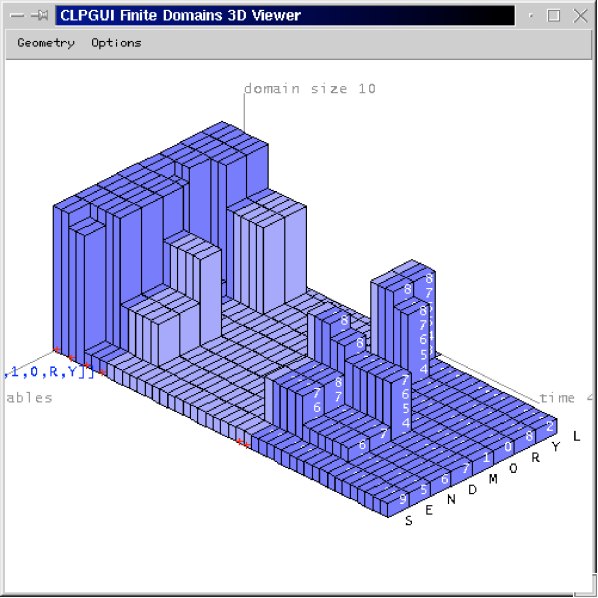
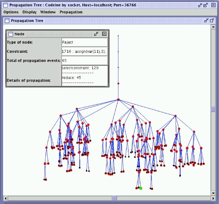
Figure 8: Two trace-based views based on the pattern visu_cstr of Figure 7.

Fig. 7 presents five patterns that can be activated simultaneously. The first three patterns are visualization oriented: the first one, visu_tree, aims at constructing the search-tree (creation of a choice-point, backtracking, failure and solution are the relevant ports) with few details about each node: the label of the node, its depth and the chronological time stamp of the event. This enables the display of nodes to be weighted by the time spent in their sub-tree.

The second pattern, visu_cstr, requests the trace of each constraint-posting with the identifier of the constraint (a unique integer), its representation (the name of the constraint with its parameters) and the list of the involved variables (varC). Fig. 8 gives two screen-shots of visualizations that are built using pattern visu_cstr. The first picture is generated by CLPGUI [Fages (2002)]. The second picture is generated by Pavot, a graphical tool developed at INRIA Rocquencourt and connected to GNU-Prolog tracer driver .

The third pattern, visu_prop, requests the trace of all the domain reductions made by constraints that do not come from the assignment procedure and that do not remove the maximal integer value. It stores the reducing constraint and the reduced variable. Those data can be used to compute some statistics and to visualize the impact of each constraint on its variables. Those three patterns are asynchronous: the requested data are sufficient for the visualization and the patterns do not have to be modified.

The fourth pattern, leaf, synchronizes the execution at each leaf of the search-tree (solution or failure). At those events, the new_leaf function can interact with the tracer to investigate the execution state.

The last pattern, symbolic, is more monitoring-oriented: it freezes the execution at each domain reduction made by a symbolic constraint such as element (on variables) or exactly. This pattern allows the monitoring of the filtering algorithms used for these two constraints.

4 Analyzer Mediator

The analyzer mediator is the interface between the tracer driver and the analyzers. It specifies to the tracer driver what events are needed and may execute specific actions for each class of relevant events. The mediator can supervise several analyses at a time. Each analysis has its own purpose and uses specific pieces of trace data. The independence of the concurrent analyses is ensured by the mediator that centralizes the communication with the tracer driver and distributes the trace data to the ongoing analyses. The advantage is that if a piece of trace information is needed by several analyses, it is sent over the interface only once.

When a synchronous event has been sent to the mediator, the requests that an analyzer can send to the driver are of three kinds. Firstly, the analyzer can ask for additional data about the current event. Secondly, the analyzer can modify the set of active event patterns, to be checked by the tracer driver. Thirdly, the analyzer can notify the tracer driver that the execution can be resumed. The actual requests are as follows.

current specifies a list of event attributes to retrieve in the current execution event. The tracer retrieves the requested pieces of data. It sends the data as a list of pairs $(attribute,value)$.

reset deletes all the active event patterns and their labels.

remove deletes the active patterns whose labels are specified in the parameter.

add inserts in the active patterns, the event patterns specified in the parameter, following the grammar described in Figure 6.

go notifies the tracer driver that the traced execution is to be resumed.

step :-
  reset,
  add([step:when true dosynchro call(tracer_toplevel)]),
  go.

skip_reductions :-
  current(cstr = CId and port = P),
  reset,
  (  P == awake
  -> add([sr:when cstr = CId and port in [suspend,reject,entail]
                    dosynchro call(tracer_toplevel)]),
  ;  add([step:when true do_synchro call(tracer_toplevel)])
  ),
  go.

Figure 9: Implementation of two tracing commands

Fig. 9 illustrates the use of the primitives to implement two tracing commands. Let us assume that the analyzer is a (possibly simplified) Prolog interpreter, as for example in Opium [Ducassé (1999b)]. Command step enables execution to go to the very next event. It simply resets all patterns and adds one that will match any event and call, with synchronous interactions, the tracer toplevel. Command skip_reductions enables execution to skip the details of variable domain reductions when encountering the awakening of a constraint. It first checks the current port. If it is awake it asks to go to the suspension of this constraint. There, the user will, for example, be able to check the value of the domains after all the reductions. If the command is called on an event of another type, it simply acts as step.

5 Filtering Mechanism

This section describes in detail the critical issue of the filtering mechanism. At each execution event, it is called to test the relevance of the event with respect to the active patterns. Notice that the execution of a program with constraints can lead to several millions of execution events per second. Therefore, the efficiency of the event filtering is a key issue.

In the following, we first describe the algorithm of the tracer driver. Then we specify the automata which drive the matching of events against active patterns. We discuss some specialisation issues. We give some details about the incremental handling of patterns. Lastly, we emphasize that event attributes are computed only upon demand.

5.1 Tracer Driver Algorithm

 1.  proc tracerDriver($P:$ set of active patterns)
 2.    $tagged\leftarrow\emptyset$
 3.    for each p $\in P$ do
 4.     if match(p) then $tagged\leftarrow tagged\cup\{p\}$
 5.    end for
 6.   T $\leftarrow\{requested\_data(p)|p\in\mathrm{tagged}\}$
 7.   send_trace_data(T, $label(tagged)$)
 8.   if $synchronous(tagged)\neq\emptyset$ then
 9.     notify($synchronous(tagged)$)
10.     repeat
11.        $request$ $\leftarrow$ receive_from analyzer()
12.        execute($request$)
13.     until $request$ = $\mathbf{go}$
14.    end if
15.  end proc

Figure 10: Algorithm of the Tracer Driver

When an execution event occurs, the tracer is called. The tracer collects some data to maintain its own data structures and then calls the tracer driver. The algorithm of the tracer driver is given in Fig. 10. The filtering mechanism can handle several active event patterns. For each pattern, if the current event matches the pattern the latter is tagged as activated; whatever the matching result, the next pattern is checked (lines 3-5). When no more patterns have to be checked, the tagged patterns are processed; the union of requested pieces of data is sent as trace data with the labels of the tagged patterns (lines 6-7). If at least one synchronous pattern is tagged, a signal is sent to the analyzer; the tracer driver waits for requests coming from the analyzer and processes them until the $\mathbf{go}$ primitive is sent by the analyzer (lines8-14).

5.2 Pattern Automata

The matching of an event against a pattern is driven by an automaton where each state is labeled by an elementary condition with two possible transitions: true or false. The automaton has two final states, $\mathbf{true}$ and $\mathbf{false}$. If the $\mathbf{true}$ state is reached, the event is said to match the pattern. Each automaton results from the compilation of an event pattern. This compilation is inspired by the evaluation of Boolean expressions in imperative languages. It has been proven that it minimizes the number of conditions to check [Wilhelm and Maurer (1995)]. Examples of automata are given in Figure 11, section 5.4.

5.3 Specialization According to the Port

As seen in Section 3, the port is a special attribute since it denotes the type of the execution event being traced. A port corresponds to specific parts of the solver code where a call to a function of the tracer has been hooked. For example, in the tracer we use, there are four hooks for the reduce port, embedded into four specific functions that make domain reductions in four different ways. Furthermore, specific attributes depend on the port. As a consequence, the port is central in the pattern specification. For most patterns, a condition on the port will be explicit. When an event occurs, it is useless to call the tracer driver if no pattern is relevant for the port of this event. Therefore, for each port, a flag in the related hooks indicates whether the port appears in at least one pattern. This simple mechanism avoids useless calls to the tracer driver.

5.4 Examples of Pattern Automata

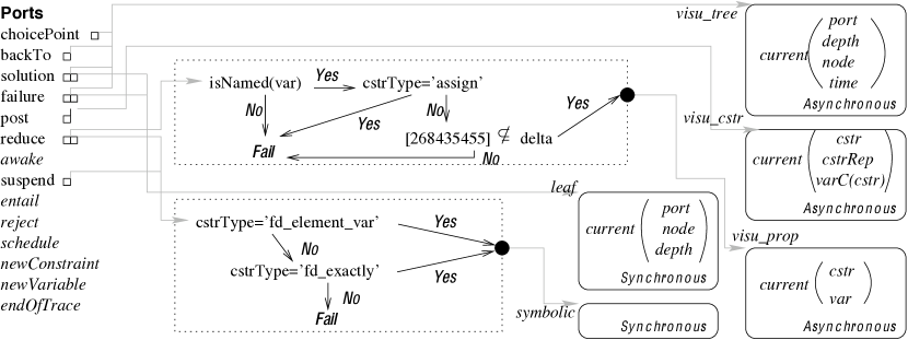
Figure 11: Internal representation of the five patterns of Figure 7

Fig. 11 shows the internal representation of the five patterns presented in Figure 7, Section 3.4. The 14 ports are represented on the left-hand side. The irrelevant ports are in italic. The relevant ports are linked to their corresponding patterns. Only two automata are necessary since three of the patterns check the port only. A set of actions is assigned to each automaton. This set is attached to “synchronous” or “asynchronous” and the label of the pattern.

5.5 Incremental Pattern Management

Since each active pattern is a specific automaton (or a list of specific automata when split), the add primitive has just to compile the new $n$ patterns into $m$ automata, linked them with their respective ports and store the labels with the lists of resulting automata. The remove primitive has just to delete the automata associated to the specified labels and to erase the dead links. After each operation, the port-filtering flags are updated so as to take into account the new state of the active patterns.

6 Prototype Implementation

In this Section, we briefly present the prototype implementation. In particular, in order for the overall architecture to be efficient, it is essential that the tracer is lazy.

Trace information must not be computed if it is not explicitly required by a pattern. Indeed, an execution has many events and events potentially have many attributes. Most of them are not straightforwardly available, they have to be computed from the execution state or from the debugging data of the tracer. Systematically computing all the attributes at all the execution events would be terribly inefficient.

Fortunately, not all the attributes need to be computed at each event. According to the active patterns, only a subset of the attributes is needed: firstly, the attributes necessary to check the relevance of the current event with respect to the patterns, and secondly, the attributes requested by the patterns in case of matching. Therefore, the tracer must not compute any trace attribute before it is needed. When a specific attribute is needed, it is computed and its value is stored until the end of the checking of the current event. If an attribute is used in several conditions, it is computed only once.

The tracer implemented in the current prototype, Codeine, strictly follows this guideline. Some core tracer mechanisms are needed to handle the debugging information (see [Langevine et al. (2003)] for more details). As shown in Sec. 7, the overhead induced by these mechanisms is marginal, even though constraint solvers do manipulate large and complex data.

Currently, Codeine is implemented in 6800 lines of C including comments. The tracer driver, including the communication mechanisms, is 1700 lines of C. The codeine tracer including the tracer driver is available under GNU Public Licence. The set of debugging and visualization tools called Pavot has been developed by Arnaud Guillaume and Ludovic Langevine. Both systems are available on line.

7 Experimental Results

This section assesses the performance of the tracer driver and its effects on the cost of the trace generation and communication. Sections 7.1 and 7.2 describe the methodology of the experiments and the experimental setting. Section 7.3 lists the benchmark programs. Sections 7.4, 7.5 and 7.6 respectively discuss the tracer overhead, the tracer driver overhead and the communication overhead.

7.1 Methodology of the Experiments

When tracing a program, some time is spent in the program execution ($T_{prog}$), some time is spent in the core mechanisms of the tracer ($\Delta_{tracer}$), some time is spent in the tracer driver ($\Delta_{driver}$), some time is spent generating the requested trace and sending it to the analysis process ($\Delta_{gcom}$), and lastly some time is spent in the analyses ($\Delta_{ana}$). Hence, if we call $T$ the execution time of a traced and analyzed program, we approximately have:

$T\simeq T_{prog}+\Delta_{tracer}+\Delta_{driver}+\Delta_{gcom}+\Delta_{ana}$.

The mediator is a simple switch. The time taken by its execution is negligible compared to the time taken by the simplest analysis, namely the display of trace information. Trace analysis takes a time which can vary considerably according to the nature of the analysis. The focus of this article is not to discuss which analyses can be achieved in reasonable time but to show that a flexible analysis environment can be offered at a low overhead. Therefore, in the following measurements $\Delta_{ana}=0$.

7.2 Experimental Setting

The experiments have been run on a PC, with a 2.4 GHz Pentium iv, 512 Kb of cache, 1 Gb of RAM, running under the GNU/Linux 2.4.18 operating system. We used the most recent stable release of GNU-Prolog (1.2.16). The tracer is an instrumentation of the source code of this version and has been compiled by gcc-2.95.4. The execution times have been measured with the GNU-Prolog profiling facility whose accuracy is said to be 1 ms. The measured executions consist of a batch of executions such that each measured time is at least 20 seconds. The measured time is the sum of system and user times. Each experimental time given below is the average time of a series of ten measurements. In each series, the maximal relative deviation was smaller than 1 %.

7.3 Benchmark Programs

The 9 benchmark programs are listed in Table 1, sorted by increasing number of trace events. Magic(100), square(4), golomb(8) and golfer(5,4,4) are part of CSPLib, a benchmark library for constraints by Gent and Walsh [Gent and Walsh (1999)]. The golomb(8) program is executed with two strategies which exhibit very different response times. Those four programs have been chosen for their significant execution time and for the variety of constraints they involve. Four other programs have been added to cover more specific aspects of the solver mechanisms: Pascal Van Hentenryck’s bridge problem, implementation of [Diaz (2003)]; two instances of the $n$-queens problem; and “propag”, which proves the infeasibility of

$$1\leq x\wedge y\leq 70000000\wedge x<y\wedge y<x.$$

The interest of the latter is the long stage of propagation involving one of the simplest and the most optimized constraints GNU-Prolog provides: bound consistency for a strict inequality. Therefore, this program the worst kind of case for the propagation instrumentation.

Program	#events	Trace	$T_{prog}$	$\varepsilon$	$R_{tr.}$	Dev.
	($10^{6}$)	Size	$(ms)$	$(ns)$		for $T_{x}$
		(Gb)				in %
bridge	0.2	0.1	14	72	1.21	$\leq 0.4$
queens(256)	0.8	1.5	173	210	1.14	$\leq 0.2$
magic(100)	3.2	1.4	215	66	1.03	$\leq 0.2$
square(24)	4.2	20.8	372	88	1.05	$\leq 0.6$
golombF	15.5	3.4	7,201	464	1.01	$\leq 0.4$
golomb	38.4	7.9	1,721	45	1.00	$\leq 0.5$
golfer(5,4,4)	61.0	>30	3,255	53	1.05	$\leq 0.7$
propag	280.0	>30	3,813	14	1.28	$\leq 1.0$
queens(14)	394.5	>30	17,060	43	1.08	$\leq 0.4$

Table 1: Benchmark Programs and tracer overhead

The benchmark programs have executions large enough for the measurements to be meaningful. They range from 200,000 events to about 400 millions events. Furthermore, they represent a wide range of CLP(FD) programs.

The third column gives the size of the traces of the benchmarked programs for the default trace model. All executions but the smallest one exhibit more than a gigabyte, for executions sometimes less than a second. It is therefore not feasible to systematically generate such an amount of information. As a matter of fact measuring these sizes took us hours and, in the last three cases, exhausted our patience! Note that the size of the trace is not strictly proportional to the number of events because different sets of attributes are collected at each type of events. For example, for domain reductions, several attributes about variables, constraints and domains are collected while other types of events simply collect the name of the corresponding constraint.

The fourth column gives $T_{prog}$, the execution time in $ms$ of the program simply run by GNU-Prolog. The fifth column shows the average time of execution per event $\varepsilon=\frac{T_{prog}}{\mathrm{\#events}}$. It is between 14 ns and 464 ns per event. For most of the suite $\varepsilon$ is around 50ns. The three notable exceptions are propag ($\varepsilon=14$ ns), queens(256) ($\varepsilon=210$ ns) and golombF ($\varepsilon=464$ ns). The low $\varepsilon$ is due to the efficiency of the propagation stage for the constraints involved in this computation. The large $\varepsilon$s are due to a lower proportion of “fine-grained” events.

7.4 Tracer Overhead

The sixth column of Table 1 also gives the results of the measurements of the overhead of the core tracer mechanisms, $R_{tr(acer)}$, which is defined as the ratio:

$R_{tr(acer)}=\frac{T_{tracer}}{T_{prog}}$.

where the measure of

$T_{tracer}\simeq T_{prog}+\Delta_{tracer}$

is the execution time of the program run by the tracer without any pattern activated. The tracer maintains its own data for all events. However, no attribute is calculated and no trace is generated.

The seventh column gives the maximum deviation for $T_{prog}$ and $T_{tracer}$.

Core tracer mechanisms can be permanently activated. 

For all the measured executions $R_{tracer}$ is less than 30% in the worst case, and less than 5% for five traced programs. The results for $R_{tracer}$ are very positive; they mean that the core mechanisms of the tracer can be systematically activated. Users will hardly notice the overhead. Therefore, while developing programs, users can directly work in “traced” mode; they do not need to switch from untraced to traced environments. This is a great comfort. As soon as they need to trace they can immediately get information.

7.5 Tracer Driver Overhead

The measure of $T_{driver}\simeq T_{prog}+\Delta_{trace}+\Delta_{driver}$ is the execution time of the program run by the tracer with the filtering procedure activated for generic patterns. Only the attributes necessary for the requested patterns are calculated at relevant events. In order for $\Delta_{gcom}$ to be zero, the patterns are designed such that no event matches them. One run is done per pattern. The patterns are listed in Figure 12. Pattern 1a is checked on few events and on one costly attribute only. Pattern 2a is checked on two costly attributes and on numerous events. Indeed, reduce events trace the main mechanism of the propagation and they are significantly more numerous than the other types of events. Pattern 3a is checked on all events and on one cheap attribute. Pattern 4a is checked on all events and systematically on three attributes.

1a. when port=post and isNamed(cname)
     do current(port,chrono,cident).

2a. when port=reduce and
           (isNamed(vname) and isNamed(cname))
     do current(port,chrono,cident).

3a. when chrono=0 do current(chrono).

4a. when depth=50000 or (chrono>=1 and node=9999999)
     do current(chrono,depth).

5a: patterns 1a, 2a, 3a and 4a activated simultaneously.

Figure 12: Patterns used to measure the tracer driver overhead

Figure 13: Cost of the tracer driver mechanisms for patterns 1a to 5a compared to $\mathbf{\varepsilon}$

Figure 14: Cost of the tracer driver mechanisms compared to the number of events

In order to measure the overhead of the tracer driver, for each of the 5 patterns a ratio $R_{pattern}$ is computed for all benchmark programs :

$R_{pattern}=\frac{T_{driver}}{T_{prog}}=1+\frac{\Delta_{driver}^{pattern}}{T_{prog}}$.

Figure 13 displays all the ratios compared to the average time per event ($\varepsilon$) of the programs. The smallest value of $\varepsilon$, 14, corresponds to program propag and the biggest value, 464, corresponds to program golombF.

In addition, the figure shows the curve $Sigma\;R=R_{1a}+R_{2a}+R_{3a}+R_{4a}-3$, that adds the overheads of the four separated patterns.

Tracer driver overhead is acceptable. 

In Figure 13, for all but one program, $R_{pattern}$ is negligible for the very simple patterns and less than 3.5 for pattern 5a which is the combination of the other four patterns. For programs with a large $\varepsilon$, even searching for pattern 5a is negligible. In the worst case, for propag, an overhead ratio of 8 is still acceptable.

No overhead for simultaneous search for patterns. 

When $n$ patterns are checked simultaneously they already save $(n-1)T_{tracer}$ compared to the search in sequence which requires the program to be executed $n$ times instead of one time. Figure 13 further shows that the curve $Sigma\;R=R_{1a}+R_{2a}+R_{3a}+R_{4a}-3$, is above the curve of $R_{5a}$. Hence

$\Delta_{driver}^{1a}+\Delta_{driver}^{2a}+\Delta_{driver}^{3a}+\Delta_{driver}^{4a}>\Delta_{driver}^{(1|2|3|4)a}$.

This means that not only is there no overhead in the filtering mechanism induced by the simultaneous search, but there is even a minor gain, due to the factorization in the automata described Section 5.2.

Tracer driver overhead is predictable. 

The measured points of Figure 13 can be interpolated with curves of the form

$R_{driver}=a+b/\varepsilon$.

Figure 14 recalls the curve for pattern 5a and gives the number of events. It shows that there is no correlation between the size of the trace and the tracer driver overhead.

Those results mean that the tracer and tracer driver overheads per event can be approximated to constants depending on the patterns and these constants are independent of the traced program. Indeed, let us assume that that $\Delta_{tracer}=N\delta_{tracer}$ and $\Delta_{driver}=N\delta_{driver}$ where $N$ is the number of events of an execution, $\delta_{tracer}$ and $\delta_{driver}$ are the average time per event taken respectively by the core tracer mechanism and the tracer driver, for all the programs. We have also already assumed that

$T_{driver}\simeq T_{prog}+\Delta_{tracer}+\Delta_{driver}$,

and we have

$R_{driver}=\frac{T_{driver}}{T_{prog}}$,   and   $T_{prog}=N\varepsilon$

therefore

$R_{driver}\simeq\frac{T_{prog}+\Delta_{tracer}+\Delta_{driver}}{T_{prog}}$

$R_{driver}\simeq 1+\frac{N(\delta_{tracer}+\delta_{driver})}{N\varepsilon}$

$R_{driver}\simeq 1+\frac{\delta_{tracer}+\delta_{driver}}{\varepsilon}$

The measured $R_{driver}$ for pattern 5a is

$R_{driver}=0.95+\frac{100ns}{\varepsilon}$.

For pattern 5a, the average time per event taken by the core tracer mechanism and the tracer driver ($\delta_{tracer}+\delta_{driver}$) can therefore be approximated to $100ns$.

The $R_{driver}$ overhead could thus be made predictable. For a given program, it is easy to automatically measure $\varepsilon$, the average time of execution per event. For a library of patterns $\delta_{tracer}+\delta_{driver}$ can be computed for each pattern. We have shown above that the overhead of the simultaneous search for different patterns can be over approximated by the sum of all the overheads. Our environment could therefore provide estimation mechanisms. When $\varepsilon$ would be too small compared to $\delta_{tracer}+\delta_{driver}$ the user would be warned that the overhead may become large.

7.6 Communication Overhead

The measure of

$T_{gcom}\simeq T_{tracer}+\Delta_{driver}+\Delta_{gcom}$

is the execution time of the program run by the tracer. A new set of patterns are used so that some events match the patterns, the requested attributes of the matched events are generated and sent to a degenerated version of the mediator: a C program that simply reads the trace data on its standard input. We show the result of program golomb(8) which has a median number of events and has a median $\varepsilon$.

6b. cstr: when port=post do current(chrono,cident,cinternal).
     tree: when port in [failure,backTo, choicePoint,solution] do current(chrono,node,port).

7b. newvar: when port=newVariable do current(chrono, vident, vname).
     dom: when port in [choicePoint,backTo,solution]
            do current(chrono,node,port,named_vars,full_dom).

8b. propag1: when port=reduce do current(chrono).

9b. propag2: when port=awake do current(chrono).

Figure 15: Event patterns used to assess the trace generation and the communication overhead

The patterns are listed in Figure 15. Pattern 6b, composed of two basic patterns, allows a “bare” search tree to be constructed, as shown by most debugging tools. Pattern 7b (two basic patterns) allows the display of 3D views of variable updates as shown in Figure 8. Pattern 8b and pattern 9b provide two different execution details to decorate search trees. Depending on the tool settings, three different visual clues can be displayed. One is shown in Figure 8, Section 3.4.

Program: golomb(8)  $\varepsilon=45\mathrm{ns}$  $T_{prog=1.73\mathrm{s}}$
Patterns	Matched	XML Trace	Elapsed	$R_{driver}$	$R_{gcom}$
	events	size	time
	$(10^{6})$	(Mbytes)	(s)
6b	0.36	21	4.50	1.03	2.6
7b	0.13	111	16.17	1.02	9.35
8b	5.04	141	33.57	1.14	19.40
9b	14.58	394	89.40	1.32	51.68
(6|7)b	0.36	124	17.47	1.04	10.09
(6|8)b	5.40	162	36.08	1.15	20.85
(6|9)b	14.94	415	92.71	1.33	53.59
(6|8|9)b	19.97	556	122.72	1.44	70.93
(6|7|8|9)b	19.97	660	136.80	1.44	79.07
default trace	38.36	7,910	393.08	1.96	227.21

Table 2: Cost of the trace generation and communication for program golomb(8)

Table 2 gives the results for the above patterns and some of their combinations. All combinations correspond to existing tools. For example, combining 6b with 8b or/and 4b allows a Christmas tree as shown in Figure 8 to be constructed with two different parametrization. The 2^nd column gives the number of events which match the pattern. The 3^rd column gives the size of the resulting XML trace as it is sent to the tool. The 4^th column gives the elapsed time. The 5^th column gives the ratio $R_{driver}$, recomputed for each pattern. The 6^th column gives the ratio $R_{gcom}=\frac{T_{gcom}}{T_{prog}}$.

Filtered trace is more efficient and more accurate than default trace. 

The last line gives results for the default trace. On the one hand, the default trace contains twice as many events as the trace generated by pattern (6|7|8|9)b; it also contains more attributes than requested by the pattern; as a result, its size is ten times larger and its $R_{gcom}$ overhead is three times larger. On the other hand, the default trace does not contain all the attributes. In that particular case, some relevant attributes are missing in the default trace while they are present in the trace generated by pattern (6|7|8|9)b. These attributes can be reconstructed by the analysis module, but this requires further computation and memory resources.

As a consequence, the tracer driver approach that we propose is more efficient than sending over a default trace, even to construct sophisticated graphical views. The accuracy and the lower volume of the trace ease its post-processing by the debugging tools.

Answering queries is more efficient than displaying traces. 

$R_{gcom}$ is always much larger than $R_{driver}$, from $2.6$ to $79.07$ in our example. Therefore, queries using patterns that drastically filter the trace have significantly better response time than queries that first display the trace before analyzing it.

When debugging, programmers often know what they want to check. In that case they are able to specify queries that demand a simple answer. In such a case our approach is significantly better than systematically sending the whole trace information to an analyzer.

No need to restrict the trace information a priori. 

Many tracers restrict the trace information a priori in order to reduce the volume of trace sent to an analyzer. This restricts the possibilities of the dynamic analyses without preventing the big size and time overhead as shown above with the default trace which does not contain important information while being huge.

With our approach, trace information which is not requested does not cost much, therefore our trace model can afford to be very rich. This makes it easier to add new dynamic analyses.

Performance is comparable to the state-of-the-practice. 

$R_{gcom}$ varies from 2.6 to 79.07. To give a comparison, the Mercury tracer of Somogyi and Henderson [Somogyi and Henderson (1999)] is regularly used by Mercury developers. For executions of size equivalent to those of our measurements, the Mercury tracer overhead has been measured from 2 to 15, with an average of 7 [Jahier and Ducassé (2002)]. Hence the ratios for patterns 6b, 7b and 6|7b are quite similar to the state-of-the-practice debuggers. The other patterns show an overhead that can discourage interactive usage. However, these patterns are thought of more for monitoring than debugging when the interaction does not have to be done in real time. Note, furthermore, that for the measured programs, the absolute response time is still on the range of two minutes for the worst case. When debugging, this is still acceptable, especially if one considers that in the relevant cases the alternatives to the uses of tools like ours are likely to be much worse.

Our approach therefore allows to have the tracer present but idle by default. When a problem is encountered, simple queries can be set to localize roughly the source of the problem. Then, more costly patterns can be activated on smaller parts of the program. This is similar to what experienced programmers do. The difference with our approach is that they do not have to either change tools, or reset the parametrization of the debugger.

8 Related Work

Kraut [Bruegge and Hibbard (1983)] implements a finite state machine to find sequences of execution events that satisfy some patterns, called path rules. Several patterns are allowed and they can be enabled or disabled during the execution, using a labeling policy. Specified actions are triggered when a rule is satisfied but they are limited to some debugger primitives, such as a message display or incrementing a counter. The main interest of this tool is to abstract the trace and to allow the easy development of monitors. The trace analysis is necessarily synchronous and does not benefit from the power of a complete programming language.

Reiss and Renieris [Reiss and Renieris (2001)] have an approach similar to ours. They also structure their dynamic analyses into three different modules: 1) extraction of trace, 2) compaction and filtering and 3) visualization. They provide a number of interesting compaction functions which should be integrated in a further version of our system. They, however, first dump the whole trace information in files before any filtering is processed. With our tracer driver, filtering is done on the fly, and Section 7 has shown that this is much more efficient than first storing in files. Their approach, however, is able to deal with partially ordered execution threads; adapting our framework to languages with partially ordered threads would require some technical work.

Coca [Ducassé (1999b)] and Opium [Ducassé (1999b)] provide a trace query mechanism, respectively for C and Prolog. This mechanism is synchronous and does not allow concurrent analyses. It can be easily emulated with our tracer driver and an analyzer mediator written in Prolog.

Hy⁺ [Consens et al. (1994)] writes the trace into a real relational database to query it with SQL. This is even slower than writing the trace simply into a file. However, when on the fly performance is not an issue, for example for post mortem analysis, this is a very powerful and elegant solution which is straightforward to connect to a tracer with our tracer driver.

Dalek [Olsson et al. (1990)] is a powerful extension of gdb. It allows users to associate sequences of execution events to specific synchronous handlers written in a dedicated imperative language. This language includes primitives to retrieve additional trace data and to synchronize the execution. The management of handlers is not incremental. A key feature of Dalek, especially useful in an imperative language, is the explicit “queue of events” that stores the achieved execution events. The user can explicitly remove events from this queue and add higher-level events. This approach requires an expensive storage of a part of the trace but enables both monitoring, debugging and profiling of programs.

In EBBA [Bates (1995)], expected program behaviors are modeled as relationships between execution events. Those models are then compared to the actual behavior during execution. EBBA tries to recognize relevant sequences of events and to check some constraints about such sequences. A kind of automaton is built to find instantiations of the models. The events are first generated by the tracer before being filtered according to the automata. Our approach allows filtering execution events directly inside the tracer, which is more efficient. Nevertheless, EBBA recognizes sequences of events whereas we filter one event at time. Our approach could be used upstream of the sequence recognition. The incrementality of the event patterns could be used to adapt the relevant events to the states of the automata.

UFO [Auguston et al. (2002)] offers a more powerful language to specify patterns and monitors than EBBA. The patterns can involve several events, not necessarily consecutive. In our framework, the monitors have to be implemented in the analyzer with a general programming language. A further extension should allow at least the implementation of monitors in the trace driver to improve efficiency. UFO, however, does not allow the same flexibility as our tracer driver, and is heavier to use for interactive debugging.

So far, our framework applies only to a single execution and does not easily scale to compare numerous executions as is done in “batch mode” by  [Jones et al. (2002)]. It seems, however, possible to extend our framework so that two executions can be run in parallel with two tracer drivers. This would allow the implementation of the debugging analyses of [Zeller and Hildebrandt (2002)] and [Sosic and Abramson (1997)] which compare two executions at a given moment.

For some applications, it is important to be able to rewind the execution. The necessary mechanisms are orthogonal to the ones presented here, and can be merged with them. Interested readers are referred to the Mercury mechanisms [MacLarty and Somogyi (2006)] or the survey of [Ronsse et al. (2000)].

The Ilog Christmas Tree [Bracchi et al. (2001)] is built by processing an XML trace produced by the debugger. This tracer is generic: it can be specialized to feed a specific tool. This specialization requires, however, a good understanding of the solver behavior and cannot be modified during the execution. Moreover, the amount of data available at each event is very limited compared to the full state our approach allows. For instance, the set of constraints and variables cannot be inspected.

A debugging library for SICStus Prolog has been implemented [Ågren et al. (2002), Hanák et al. (2004)]. Its main quality is the explanations it provides about events that narrow domains. This helpful information needs a difficult and costly instrumentation of SICStus constraints: only a few ones have actually been instrumented. No performance results are available. Some tuning of the trace display is possible but the tracer is based on a complete storage of the trace and a postmortem investigation: this is impractical with real-sized executions. The lazy generation of the trace our tracer driver enables leads to the same kind of trace data in a more efficient and practical way.

Some C(L)P debugging tools enable users to interact with the execution states. User of Oz Explorer [Schulte (1997)] can act on the current state of the execution to drive the search-tree exploration. Users of CLPGUI [Fages (2002)] can add new constraints on a partial solution. They can recompute a former state in both systems. Those features are helpful. Our approach is complementary, it addresses the communication from the traced execution to the debugging tools.

9 Conclusion

In this paper we have presented a tracer driver which, with limited development efforts, provides a powerful front-end for complex debugging and monitoring tools based on trace data.

We have defined an expressive language of event patterns where relevant events are described by logical formulæ involving most of the data the tracer can access. Specific primitives enable the retrieval of large pieces of data “on demand” and the adaptation of the event patterns to the evolving needs of trace analyzers.

Experiments for CLP(FD) have shown that the overhead of the core tracer mechanisms is small, therefore the core tracer can be permanently activated; the tracer driver overhead is acceptable; there is no overhead in the filtering mechanisms when searching simultaneously for several patterns; the tracer driver overhead is predictable for given patterns; the tracer driver approach that we propose is more efficient than sending over a default trace, even to construct sophisticated graphical views; answering queries is orders of magnitude more efficient than displaying traces; there is no need to restrict the trace information a priori; last but not least, the performance of our tool is comparable to the state-of-the-practice while being more powerful and more generic.

Traditionally, tracer designers decide on a static basis what the observed events should be. As a result, compromises regarding the amount of information to trace are made once for all or, at best, before each execution. With our approach the trace contents can be much richer because only what is needed is retrieved. Hence there is less chance that important information is missing.

The tracer driver overhead is inversely proportional to the average time between two traced events. Whereas the principles of the tracer driver are independent of the traced programming language, it is best suited for high-level languages, such as constraint logic programming, where each traced execution event encompasses numerous low-level execution steps.

The current C(L)P environments do not provide all the useful dynamic analysis tools. They can significantly benefit from our tracer driver which enables dynamic analyses to be integrated at a very low cost.

Acknowledgment

The authors thank Pierre Deransart and their OADymPPaC partners for fruitful discussions, as well as Guillaume Arnaud for the screenshots of his Pavot tool and his careful beta-testing of Codeine. Ludovic Langevine is indebted to Mats Carlsson and the SICStus team at Uppsala who helped to implement a preliminary tracer driver prototype connected to the FDBG SICStus Prolog tracer [Ågren et al. (2002)]. It contributed to the validation of the principles described in this article.

References

- Ågren et al. (2002) Ågren, M., Szeredi, T., Beldiceanu, N., and Carlsson, M. 2002. Tracing and explaining execution of clp(fd) programs. In Proc. of Workshop on Logic Programming Environments’02, A. Tessier, Ed. Computer Research Repository cs.SE/0207047.
- Auguston et al. (2002) Auguston, M., Jeffery, C., and Underwood, S. 2002. A framework for automatic debugging. In Proceedings fo the 17th International Conference on Automated Software Engineering (ASE’02), W. Emmerich and D. Wile, Eds. IEEE Press, 217–222.
- Ball (1999) Ball, T. 1999. The concept of dynamic analysis. In ESEC / SIGSOFT FSE, O. Nierstrasz and M. Lemoine, Eds. Lecture Notes in Computer Science, vol. 1687. Springer, 216–231.
- Bates (1995) Bates, P. C. 1995. Debugging heterogeneous distributed systems using event-based models of behavior. ACM Transactions on Computer Systems 13, 1 (Feb.), 1–31.
- Bracchi et al. (2001) Bracchi, C., Gefflot, C., and Paulin, F. 2001. Combining propagation information and search-tree visualization using opl studio. In Proceedings of WLPE’01, A. Kusalik, Ed. Computer Research Repository cs.PL/0111040, Cyprus, 27–39.
- Bruegge and Hibbard (1983) Bruegge, B. and Hibbard, P. 1983. Generalized path expressions: A high-level debugging mechanism. The Journal of Systems and Software 3, 265–276. Elsevier.
- Carro and Hermenegildo (2000) Carro, M. and Hermenegildo, M. 2000. The VIFID/TRIFID tool. See Deransart et al. (2000), Chapter 10.
- Consens et al. (1994) Consens, M., Hasan, M., and Mendelzon, A. 1994. Visualizing and querying distributed event traces with Hy+. In Applications of Databases, First International Conference, W. Litwin and T. Risch, Eds. Springer, Lecture Notes in Computer Science, Vol. 819, 123–141.
- Denmat et al. (2005) Denmat, T., Ducassé, M., and Ridoux, O. 2005. Data mining and cross-checking of execution traces. a re-interpretation of Jones, Harrold and Stasko test information visualization. In Proceedings of the 20th IEEE/ACM International Conference on Automated Software Engineering, T. Ellman and A. Zisman, Eds. ACM Press.
- Deransart et al. (2000) Deransart, P., Hermenegildo, M., and Maluszynski, J., Eds. 2000. Analysis and visualization tools for constraint programming. Lecture Notes in Computer Science, vol. 1870. Springer-Verlag.
- Diaz (2003) Diaz, D. 2003. Gnu Prolog, a free Prolog compiler with constraint solving over finite domains. http://gprolog.sourceforge.net/ Distributed under the GNU license.
- Ducassé (1999a) Ducassé, M. 1999a. Coca: An automated debugger for C. In Proceedings of the 21st International Conference on Software Engineering. ACM Press, 504–513.
- Ducassé (1999b) Ducassé, M. 1999b. Opium: An extendable trace analyser for Prolog. The Journal of Logic programming 39, 177–223. Special issue on Synthesis, Transformation and Analysis of Logic Programs, A. Bossi and Y. Deville (eds).
- Fages (2002) Fages, F. 2002. Clpgui: a generic graphical user interface for constraint logic programming over finite domains. In Proceedings of WLPE’02, A. Tessier, Ed. Computer Research Repository cs.SE/0207048, Copenhagen.
- Gent and Walsh (1999) Gent, I. and Walsh, T. 1999. CSPLib: a benchmark library for constraints. Tech. rep., Technical report APES-09-1999. Available from http://csplib.cs.strath.ac.uk/. A shorter version appears in the Proceedings of CP-99.
- Goualard and Benhamou (2000) Goualard, F. and Benhamou, F. 2000. Debugging constraint programs by store inspection. See Deransart et al. (2000), Chapter 11.
- Hanák et al. (2004) Hanák, D., Szeredi, T., and Szeredi, P. 2004. FDBG, the CLP(FD) debugger library of SICStus Prolog. In Proc. of Iclp’04, B. Demoen and V. Lifschitz, Eds. Poster. LNCS 3132.
- Harrold et al. (1998) Harrold, M. J., Rothermel, G., Wu, R., and Yi, L. 1998. An empirical investigation of program spectra. In Proceedings of the 1998 ACM SIGPLAN-SIGSOFT workshop on Program analysis for software tools and engineering. ACM Press, 83–90.
- Jahier and Ducassé (2002) Jahier, E. and Ducassé, M. 2002. Generic program monitoring by trace analysis. Theory and Practice of Logic Programming 2, 4-5 (July-September), 611–643.
- Jeffery and Griswold (1994) Jeffery, C. and Griswold, R. 1994. A framework for execution monitoring in icon. Software-Practice and Experience 24, 11 (November), 1025–1049.
- Jones and Harrold (2005) Jones, J. A. and Harrold, M. J. 2005. Empirical evaluation of the Tarantula automatic fault-localization technique. In Proceedings of the 20th IEEE/ACM international Conference on Automated Software Engineering. ACM Press, 273–282.
- Jones et al. (2002) Jones, J. A., Harrold, M. J., and Stasko, J. 2002. Visualization of test information to assist fault localization. In Proceedings of the 24th International Conference on Software Engineering. ACM Press, 467–477.
- Langevine et al. (2004) Langevine, L., Deransart, P., and Ducassé, M. 2004. A generic trace schema for the portability of CP(FD) debugging tools. In Recent advances in Constraint Programming, J. Vancza, K. Apt, F. Fages, F. Rossi, and P. Szeredi, Eds. Springer-Verlag, Lecture Notes in Artificial Intelligence 3010.
- Langevine et al. (2003) Langevine, L., Ducassé, M., and Deransart, P. 2003. A propagation tracer for Gnu-Prolog: from formal definition to efficient implementation. In Proc. of the 19th Int. Conf. in Logic Programming, C. Palamidessi, Ed. Springer-Verlag, Lecture Notes in Computer Science 2916.
- MacLarty and Somogyi (2006) MacLarty, I. and Somogyi, Z. 2006. Controlling search space materialization in a practical declarative debugger. In PADL, P. V. Hentenryck, Ed. Lecture Notes in Computer Science, vol. 3819. Springer, 31–44.
- MacLarty et al. (2005) MacLarty, I., Somogyi, Z., and Brown, M. 2005. Divide-and-query and subterm dependency tracking in the Mercury declarative debugger. In AADEBUG’05: Proceedings of the sixth international symposium on Automated analysis-driven debugging. ACM Press, New York, NY, USA, 59–68.
- Meier (1995) Meier, M. 1995. Debugging constraint programs. In Proceedings of the First International Conference on Principles and Practice of Constraint Programming, U. Montanari and F. Rossi, Eds. Lecture Notes in Computer Science, vol. 976. Springer-Verlag, 204–221.
- Olsson et al. (1990) Olsson, R., Crawford, R., and Ho, W. 1990. Dalek: A GNU, improved programmable debugger. In Proceedings of the Summer 1990 USENIX Conference: June 11–15, 1990. 221–232.
- Reiss and Renieris (2001) Reiss, S. and Renieris, M. 2001. Encoding program executions. In Proceedings of the 23rd International Conference on Software Engineering, M.-J. Harrold and W. Schäfer, Eds. IEEE Press, 221–230.
- Ronsse et al. (2000) Ronsse, M., Bosschere, K. D., and Chassin de Kergommeaux, J. 2000. Execution replay and debugging. In Proceedings of the International Workshop on Automated Debugging (AADEBUG2000), M. Ducassé, Ed. http://xxx.lanl.gov/abs/cs.SE/0011006.
- Schulte (1997) Schulte, C. 1997. Oz explorer: a visual constraint programming tool. In Proc. of the 14th Int. Conf. on Logic Programming, L. Naish, Ed. MIT Press, 286–300.
- Shapiro (1983) Shapiro, E. 1983. Algorithmic Program Debugging. MIT Press, Cambridge, MA. ISBN 0-262-19218-7.
- Simonis and Aggoun (2000) Simonis, H. and Aggoun, A. 2000. Search-tree visualisation. See Deransart et al. (2000), Chapter 7.
- Somogyi and Henderson (1999) Somogyi, Z. and Henderson, F. 1999. The implementation technology of the Mercury debugger. In Proceedings of the Tenth Workshop on Logic Programming Environments. Vol. 30(4). Elevier, Electronic Notes in Theoretical Computer Science. http://www.elsevier.nl/cas/tree/store/tcs/free/entcs/store/tcs30/cover.sub.sht.
- Sosic and Abramson (1997) Sosic, R. and Abramson, D. 1997. Guard: A relative debugger. Software - Practice and Experience 27, 2, 185–206.
- Wilhelm and Maurer (1995) Wilhelm, R. and Maurer, D. 1995. Compiler design. Addison-Wesley. ISBN: 0-201-42290-5.
- Zeller and Hildebrandt (2002) Zeller, A. and Hildebrandt, R. 2002. Simplifying and isolating failure-inducing input. IEEE Transactions on Software Engineering 28, 2, 183–200.