Frequentist Coverage Properties of Uncertainty Intervals for Weak Poisson Signals in the Presence of Background

Abstract

We construct uncertainty intervals for weak Poisson signals in the presence of background. We consider the case where a primary experiment yields a realization of the signal plus background, and a second experiment yields a realization of the background. The data acquisitions times, for the background-only experiment, $T_{bg}$, and the primary experiment, $T$, are selected so that their ratio, $\frac{T_{bg}}{T}$, varies from 1 to 25. The upper choice of 25 is motivated by an experimental study at the National Institute of Standards and Technology (NIST). The expected number of background counts in the primary experiment varies from 0.2 to 2. We construct 90 and 95 percent confidence intervals based on a propagation-of-errors method as well as two implementations of a Neyman procedure where acceptance regions are constructed based on a likelihood-ratio criterion that automatically determines whether the resulting confidence interval is one-sided or two-sided. In one of the implementations of the Neyman procedure due to Feldman and Cousins, uncertainty in the expected background contribution is neglected. In the other implementation, we account for random uncertainty in the estimated expected background with a parametric bootstrap implementation of a method due to Conrad. We also construct minimum length Bayesian credibility intervals. For each method, we test for the presence of a signal based on the value of the lower endpoint of the uncertainty interval. In general, the propagation-of-errors method performs the worst compared to the other methods according to frequentist coverage and detection probability criteria, and sometimes produces nonsensical intervals where both endpoints are negative. The Neyman procedures generally yield intervals with better frequentist coverage properties compared to the Bayesian method except for some cases where $\frac{T_{bg}}{T}=1$. In general, the Bayesian method yields intervals with lower detection probabilities compared to Neyman procedures. One of main conclusions is that when $\frac{T_{bg}}{T}$ is 5 or more and the expected background is 2 or less, the FC method outperforms the other methods considered. For $\frac{T_{bg}}{T}=1,2$ we observe that the Neyman procedure methods yield false detection probabilities for the case of no signal that are higher than expected given the nominal frequentist coverage of the interval. In contrast, for $\frac{T_{bg}}{T}=1,2$, the false detection probability of the Bayesian method is less than expected according to the nominal frequentist coverage.

keywords: astroparticle and particle physics, background contamination, data and error analysis, isotopic ratios, low level radiation detection, metrology and the theory of measurement, Poisson processes, signal detection, uncertainty intervals. Contributions by staff of the National Institute of Standards and Technology, an agency of the US government, are not subject to copyright.

1 Introduction

We consider experiments where instruments yield count data that can be modeled as realizations of a Poisson process with expected value $\mu_{S}+\mu_{B}$ where $\mu_{S}$ is the expected contribution due to a signal of interest, and $\mu_{B}$ is the expected contribution of a background process. That is,

$$n_{obs}\sim Poi(\mu_{S}+\mu_{B}).$$ (1)

Given the measured value $n_{obs}$ and an estimate of $\mu_{B}$ from an independent background-only experiment, we construct uncertainty intervals (confidence intervals and Bayesian credibility intervals) for $\mu_{S}$. The statistical problem we study occurs in a variety of application areas including: particle and astroparticle physics [1-9], isotopic ratio analysis (when the major isotope is large enough so that most of the variability in the ratio is due to the minor isotope) [10,11], detection of low-level radiation [12-15], and aerosol science and technology [16].

Here, we focus on the case where the signal is weak and consider the case where the ratio of the data acquisition time for the background-only measurement $T_{bg}$ and the data acquisition time for the primary experiment $T$ varies from 1 to 25. This upper value of $\frac{T_{bg}}{T}=25$ was motivated by an experimental study at the National Institute of Standards and Technology (NIST), as were the values of $\mu_{S}$ and $\mu_{B}$ that we consider. For such cases, we demonstrate that the standard propagation-of-errors (POE) method yields confidence intervals with poor coverage properties. Sometimes the POE method produces intervals where the upper and/or lower endpoints are negative. As an aside, for the special case where $\frac{T_{bg}}{T}=1$, one can construct a confidence interval for $\mu_{S}$ based on a Bessel function approach that has better coverage properties than does the POE method [16]. However, for the general case where $\frac{T_{bg}}{T}\neq 1$, this method is not applicable. Hence, we do not include the method described in [16] in our study.

In addition to the POE method, we study the relative performance of three other methods for constructing uncertainty intervals. The first method [17] is an implementation of a frequentist Neyman procedure [18] developed by Feldman and Cousins. In this method, which we refer to as the FC method, $\mu_{B}$ is assumed to be known. For each of many discrete values of $\mu_{S}$, acceptance regions are constructed based on a likelihood-ratio criterion. Given the intersection of the actual measured value with these regions, one constructs a confidence interval for $\mu_{S}$. In our studies, we estimate $\mu_{B}$ from background-only experiments. In [19], the FC method was extended to account for systematic uncertainties in $\mu_{B}$. We denote this method as the randomized Feldman Cousins (RFC) method because $\mu_{B}$ is treated as a random nuisance parameter. In this work, we implement a version of the RFC method where uncertainty in $\mu_{B}$ is due to Poisson counting statistics variation in a background-only experiment that gives a direct measurement of $\mu_{B}$. In the RFC method, we simulate realizations of the nuisance parameter $\mu_{B}$ with a parametric bootstrap method [20]. In both the FC and the RFC methods, the upper and lower endpoints are determined automatically.

We also determine the posterior probability density function (posterior pdf) for $\mu_{S}$ with a Bayesian method [21,22] following Loredo’s treatment of the same problem in [23]. Loredo did not discuss how to select the endpoints of the credibility interval. Here, given that the integrated posterior pdf has a particular value (equal to the nominal frequentist coverage probability), we determine the endpoints by minimizing the length of the credibility interval. As an aside for the special case where $\mu_{B}$ is known, Roe and Woodroofe [24] determined minimum length Bayesian credibility intervals assuming a uniform prior for $\mu_{S}$ and studied the frequentist coverage properties of their intervals.

Bayesian credibility intervals and frequentist confidence intervals are conceptually different. To illustrate, consider a one-dimensional parameter estimation problem. Frequentist confidence intervals are constructed so that, ideally, the true value of the parameter falls within the confidence interval determined from any independent realization of data with some desired coverage probability. In contrast, Bayesian credibility intervals are constructed by modeling the parameter of interest as a random variable. Given a prior probability model for the parameter of interest and a likelihood model for the data given the parameter, Bayes theorem yields the conditional probability density function of the parameter given the observed data. Based on this conditional pdf (called the posterior pdf), one constructs credibility intervals. By design, Bayesian credibility intervals are not constructed with frequentist coverage in mind. Although the conceptual foundations of frequentist and Bayesian inference are different, frequentist coverage is widely accepted as an empirical measure of the performance of not only frequentist confidence intervals but Bayesian credibility intervals as well [22,25,26]. In a highly regarded textbook on Bayesian data analysis, Gelman, Carlin, Stern and Rubin remark (page 111 of [22])

Just as the Bayesian paradigm can be seen to justify simple ‘classical’ techniques, the methods of frequentist statistics provide a useful approach for evaluating the properties of Bayesian inferences- their operating characteristics– when these are regarded as embedded in a sequence of repeated samples.

In this frequentist coverage study, we simulate realizations of data given $\mu_{S}$ and $\mu_{B}$, and quantify the probability that $\mu_{S}$ falls in the interval determined from the simulated data. In frequentist statistics, the relationship between a confidence interval and a hypothesis test is well known. We exploit this relationship and test the null hypothesis that $\mu_{S}=0$ against the alternative hypothesis $\mu_{S}>0$, based on the value of the lower endpoint of the uncertainty interval. We reject the null hypothesis if the lower endpoint is greater than 0. Thus, the probability that the lower endpoint of an interval is greater than 0 is a signal detection probability. As a caveat, we do not claim that this procedure is the most powerful test of our hypothesis.

In Section 2, we define our measurement model and describe how we determine uncertainty intervals using each of the four methods. In this study, the background parameter $\mu_{B}$ ranges from 0.2 to 2 and the signal parameter $\mu_{S}$ ranges from 0 to 20. In Section 3, we study the coverage properties of uncertainty intervals for a variety of cases. We also determine detection probabilities for a signal of interest. In general, the propagation-of-errors method performs the worst compared to the other methods according to frequentist coverage and detection probability criteria. Further, the propagation-of-errors method sometimes produces nonsensical intervals where both endpoints are negative. The Neyman procedures generally yield intervals with better frequentist coverage properties compared to the Bayesian method except for the case where $\frac{T_{bg}}{T}=1$ and there are 1 or more expected background counts in the primary experiment. In general, the Bayesian method yields intervals with lower detection probabilities compared to Neyman procedures. When $\frac{T_{bg}}{T}$ is 5 or more, the FC method yields intervals with the highest detection probabilities and best coverage properties in general. However, for $\frac{T_{bg}}{T}=1,2$ both the Neyman procedure methods yield false detection probabilities for the case of no signal that are higher than expected given the nominal frequentist coverage of the interval. In contrast, for $\frac{T_{bg}}{T}=1,2$, the false detection probability of the Bayesian method is less than expected according to the nominal frequentist coverage.

2 Measurement Model and Uncertainty Intervals

In our simulation study, we consider an experiment where a realization of the signal of interest plus background, $n_{obs}$ is observed during a time interval $T$. In a separate experiment of duration $T_{bg}$, where $\frac{T_{bg}}{T}$ varies from 1 to 25, we measure a realization of background $n_{bg}$. We denote the data as $d=(n_{obs},n_{bg})$. The expected values of $n_{obs}$ and $n_{bg}$ are $\mu_{S}+\mu_{B}$ and $\mu_{B}\frac{T_{bg}}{T}$, respectively, where $\mu_{S}$ is the expected contribution from the signal of interest, and $\mu_{B}$ is the expected contribution from the background. We model measurements of $n_{obs}$ and $n_{bg}$ as independent Poisson random variables. Hence, the likelihood function of the data is $P(d|\mu_{S},\mu_{B})$, where

$$P(d|\mu_{S},\mu_{B})=(\mu_{S}+\mu_{B})^{n_{obs}}\frac{\exp[-(\mu_{S}+\mu_{B})]}{n_{obs}!}\times$$ (2)

$$(\mu_{B}\frac{T_{bg}}{T})^{n_{bg}}\frac{\exp[-(\mu_{B}\frac{T_{bg}}{T})]}{n_{bg}!}.$$

2.1 Feldman Cousins Method

In the FC method, one determines confidence intervals with a Neyman procedure assuming exact knowledge of $\mu_{B}$. In our study, we set $\mu_{B}$ to an empirical estimate $\hat{\mu}_{B}$, where

$$\hat{\mu}_{B}=\frac{T}{T_{bg}}n_{bg}.$$ (3)

Hence, the variance of $\hat{\mu}_{B}$ is

$$VAR(\hat{\mu}_{B})=(\frac{T}{T_{bg}})\mu_{B},$$ (4)

and the standard deviation of $\hat{\mu}_{B}$ is

$$\sigma(\hat{\mu}_{B})=\sqrt{\frac{T}{T_{bg}}}\sqrt{\mu_{B}}.$$ (5)

Thus, the fractional uncertainty of the estimate of $\mu_{B}$ is

$$\frac{\sigma(\hat{\mu}_{B})}{\mu_{B}}=\sqrt{\frac{T}{T_{bg}}}\frac{1}{\sqrt{\mu_{B}}}.$$ (6)

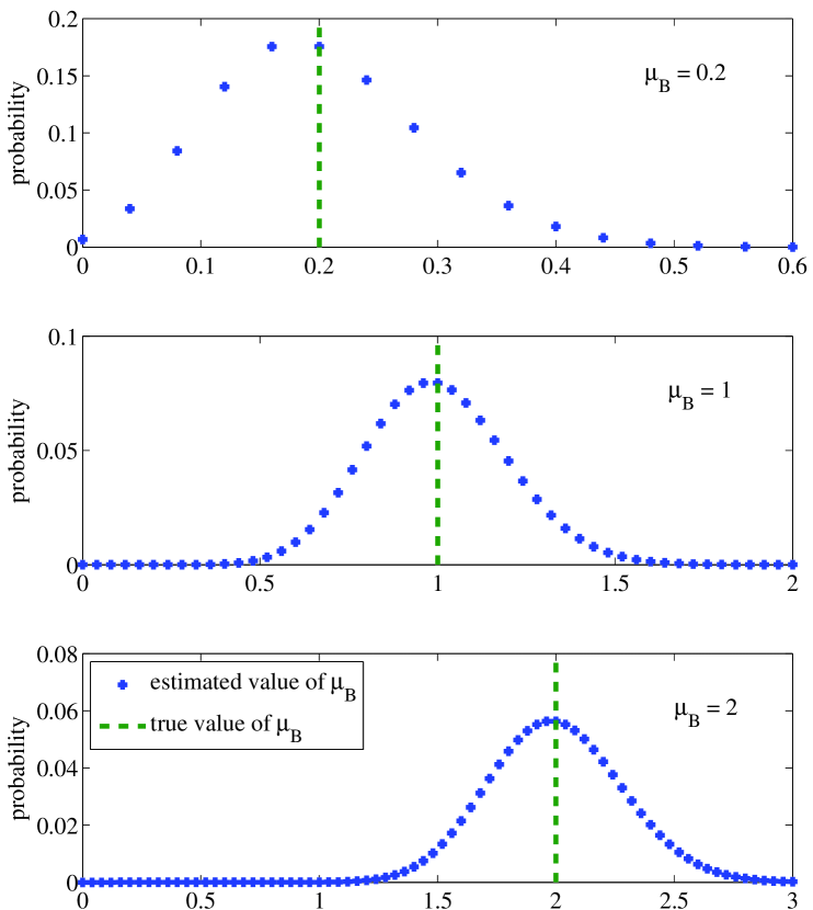
Figure 1: Probability density functions for estimated background for case where $T_{bg}/T=$ 25. For $\mu_{B}=$ 0.2, 1, and 2, the standard deviations of the estimated background are 0.09, 0.20 and 0.28 respectively. The corresponding fractional standard deviations of the estimated background are 45 $\%$, 20 $\%$, and 14 $\%$ respectively.

In Figure 1, we plot probability density functions for the estimated background when $\frac{T_{bg}}{T}=$ 25 for $\mu_{B}=$ 0.2, 1, and 2.

The FC method [17] produces a confidence interval for $\mu_{S}$ under the assumption that the assumed background ($\hat{\mu}_{B}$ in our case) equals the true background $\mu_{B}$. For various values of $\mu_{S}$, we construct an acceptance region in $n$ space. For each integer value of $n$, we compute the conditional probability $P(n|\mu_{S},\hat{\mu}_{B})$ and $P(n|\mu_{S},\hat{\mu}_{best})$, where $\hat{\mu}_{best}=max(0,n-\hat{\mu}_{B})$ and

$$P(n|\mu_{S},\hat{\mu}_{B})=(\mu_{S}+\hat{\mu}_{B})^{n}\frac{\exp[-(\mu_{S}+\hat{\mu}_{B})]}{n!}.$$ (7)

From these, we form the ratio $R$, where

$$R=\frac{P(n|\mu_{S},\hat{\mu}_{B})}{P(n|\mu_{S},\hat{\mu}_{best})}.$$ (8)

We include values of $n$ in the acceptance region with the largest values of $R$. For construction of a 100 $\times~{}p$ $\%$ confidence interval, we add values until the sum of the $P(n|\mu_{S},\hat{\mu}_{B})$ terms is $p$ or greater. The lower and upper endpoints of the confidence interval for $\mu_{S}$ are the minimum and maximum values of $\mu_{S}$ that yield acceptance regions that include the observed value $n_{obs}$. For fixed $n_{obs}$, due to the discreteness of $n$, the upper endpoint of the interval is not always a decreasing function of $\mu_{B}$. In [17], Feldman and Cousins lengthened their intervals so that the upper interval was a non-decreasing function of $\mu_{B}$. In this work, we do not adjust our intervals.

2.2 Extension of Feldman Cousins: Uncertain Background

In the RFC method, the value of $\mu_{B}$ is a random nuisance parameter. In our analysis, we assume that uncertainty in $\mu_{B}$ is due to random variation alone, i.e., counting statistics. If there were systematic error, it could be incorporated into the analysis. However, we do not do this.

The procedure to construct a confidence interval is very similar to the FC method. For each value of $\mu_{S}$, we compute an acceptance region like before, but we replace $P(n|\mu_{S},\hat{\mu}_{B})$ and $P(n|\mu_{S},\hat{\mu}_{best})$ with an estimate of their expected values when one accounts for uncertainty in $\hat{\mu}_{B}$.

One way to do this would be to simulate realizations of $\hat{\mu}_{B}$ with a parametric bootstrap [20] method and determine the mean value of $P(n|\mu_{S},\hat{\mu}_{B})$ and $P(n|\mu_{S},\hat{\mu}_{best})$ from all the realizations. In this approach, the $k$th bootstrap replication of $n_{bg}$, $n^{*}_{bg}(k)$ is simulated by sampling from a Poisson distribution with expected value equal to $n_{bg}$. That is,

$$n^{*}_{bg}(k)\sim Poi(n_{bg}).$$ (9)

Given $n^{*}_{bg}(k)$, the $k$th bootstrap replication of $\hat{\mu}_{B}$, $\hat{\mu}^{*}_{B}(k)$, is

$$\hat{\mu}^{*}_{B}(k)=\frac{T}{T_{bg}}n^{*}_{bg}(k),$$ (10)

and the $k$th bootstrap replication of $\hat{\mu}_{best}$ is $\hat{\mu}^{*}_{best}(k)=max(0,n-\hat{\mu}^{*}_{B}(k))$. Thus, the $k$th bootstrap replication of $P(n|\mu_{S},\hat{\mu})$ is

$$P(n|\mu_{S},\hat{\mu}^{*}_{B}(k))=(\mu_{S}+\hat{\mu}^{*}_{B}(k))^{n}\frac{\exp[-(\mu_{S}+\hat{\mu}^{*}_{B}(k))]}{n!},$$ (11)

and the $k$th bootstrap replication of $P(n|\mu_{S},\hat{\mu}_{best})$ is

$$P(n|\mu_{S},\hat{\mu}^{*}_{best}(k))=(\mu_{S}+\hat{\mu}^{*}_{best}(k))^{n}\frac{\exp[-(\mu_{S}+\hat{\mu}^{*}_{best}(k))]}{n!}.$$ (12)

From all $K$ bootstrap replications, we determine the following mean values

$$\bar{P}(n|\mu_{S},\hat{\mu}_{B})=\frac{1}{K}\sum_{k=1}^{K}P(n|\mu_{S},\hat{\mu}^{*}_{B}(k))$$ (13)

and

$$\bar{P}(n|\mu_{S},\hat{\mu}_{best})=\frac{1}{K}\sum_{k=1}^{K}P(n|\mu_{S},\hat{\mu}^{*}_{best}(k))$$ (14)

In this Monte Carlo implementation of the RFC method, one replaces ${P}(n|\mu_{S},\hat{\mu}_{B})$ and ${P}(n|\mu_{S},\hat{\mu}_{best})$ with the right-hand sides of Eqns. 13 and 14.

To reduce computer run time, we do not implement a Monte Carlo version of the RFC. Instead, we determine the left-hand sides of Eqns. 13 and 14 by numerical integration. For instance, we evaluate the left-hand side of Eq. 13 as

$$\bar{P}(n|\mu_{S},\hat{\mu}_{B})=\sum_{k=k_{low}}^{k_{hi}}P(n|\mu_{S},\hat{\mu}^{*}_{B}=\frac{kT}{T_{bg}})w(k)$$ (15)

where $w(k)$ is

$$w(k)=\frac{\exp(-n_{bg})n_{bg}^{k}}{k!}.$$ (16)

To speed up the algorithm, we select $k_{low}$ and $k_{hi}$ so that the sum of the $w(k)$ terms agrees with 1 to within approximately $10^{-8}$. We use a similar method to determine the left-hand side of Eq. 14.

2.3 Bayesian Method

Following [23], we determine a Bayesian credibility interval for $\mu_{S}$ given measurements of $n_{obs}$ and $n_{bg}$. In this approach, the priors $p(\mu_{B})$ and $p(\mu_{S}|\mu_{B})$ are both uniform from 0 to a large positive constant. Results are presented for the limiting case where this positive constant approaches infinity. Based on a Bayes Theorem argument, one can show that

$$p(\mu_{S},\mu_{B}|n_{obs},n_{bg})\propto p(\mu_{B}|n_{bg})p(n_{obs}|\mu_{S},\mu_{B}),$$ (17)

where the posterior pdf for $\mu_{B}$ given $n_{bg}$ is

$$p(\mu_{B}|n_{bg})=\frac{T_{bg}}{T}\frac{\exp(-\frac{T_{bg}}{T}\mu_{B})(\frac{T_{bg}}{T}\mu_{B})^{n_{bg}}}{n_{bg}!},$$ (18)

and $p(n_{obs}|\mu_{S},\mu_{B})$ is the Poisson likelihood function

$$p(n_{obs}|\mu_{S},\mu_{B})=\exp(-(\mu_{S}+\mu_{B}))(\mu_{S}+\mu_{B})^{n_{obs}}/n_{obs}!.$$ (19)

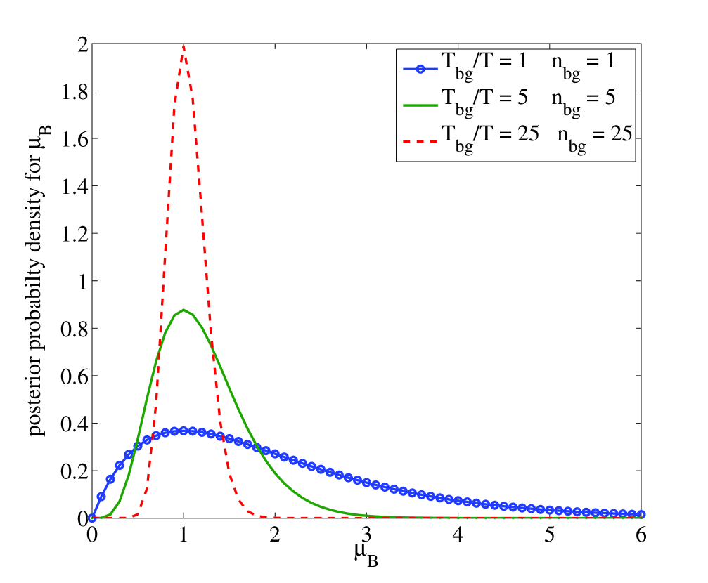
Figure 2: Posterior probability density functions for the background parameter $\mu_{B}$ given the observed value $n_{bg}$.

See Figure 2 for examples of Eq. 18.

Further, marginalizing with respect to $\mu_{B}$, we get

$$p(\mu_{S}|n_{obs},n_{bg})=\sum_{i=0}^{n_{obs}}C_{i}\frac{(\mu_{S})^{i}\exp(-\mu_{S})}{i!},$$ (20)

where

$$C_{i}=\frac{(1+\frac{T_{bg}}{T})^{i}~{}\frac{(n_{obs}+n_{bg}-i)!}{(n_{obs}-i)!}}{\sum_{j=0}^{n}(1+\frac{T_{bg}}{T})^{j}~{}\frac{(n_{obs}+n_{bg}-j)!}{(n_{obs}-j)!}}.$$ (21)

See [23] for more details of this derivation.

In this study, we determine the endpoints of 90 $\%$ and 95 $\%$ credibility intervals as follows. For both the 90 $\%$ and 95 $\%$ cases, we determine the maximum lower endpoint of the one-sided interval $l_{max}$. In an optimization code, for each trial value of the lower endpoint $l$ (where $0\leq l\leq l_{max}$) we determine the upper endpoint $u$ such that the integral of the posterior pdf from $l$ to $u$ equals the nominal frequentist coverage. We determine the lower endpoint $l$ that minimizes $u-l$. If the optimal value of $l$ is less than the specified numerical tolerance ($10^{-6}$) of the optimization algorithm, we set it to 0.

2.4 Propagation-of-Errors Method

We compute two-sided confidence intervals with a standard propagation-of-errors (POE) method that has a continuity correction. The $1-\alpha$ level POE confidence interval for $\mu_{S}$ is $\hat{\mu}_{S}\pm(z_{\alpha/2}\hat{\sigma}_{\hat{\mu}_{S}}+0.5)$ where

$$\hat{\mu}_{S}=n_{obs}-\hat{\mu}_{B},$$ (22)

and

$$\hat{\sigma}^{2}_{\hat{\mu}_{S}}=n_{obs}+(\frac{T}{T_{bg}})^{2}n_{bg}.$$ (23)

For levels of 0.90 and 0.95, $z_{\alpha/2}=$ 1.64 and 1.96, respectively. We expect that this method will yield confidence intervals with coverage close to the desired nominal values for the asymptotic case where the signal-to-noise ratio of the data is high. As a caveat, continuity corrections are typically introduced when constructing confidence intervals for the case where there is no background [27] rather than the more general case considered here.

In our simulation experiment, the POE method can yield nonsensical results where one or both endpoints are negative (Table 1). In our coverage studies, we treat negative endpoints as 0. Hence, if both endpoints are negative, the resultant interval is treated as $(0,0)$. In physics and astroparticle physics experiments where one hopes to discover a new particle, null resuls are common and experimenters provide upper limits. If both endpoints are negative, one can not set a reasonable upper limit. Hence the POE method is clearly unacceptable for low count data sets.

3 Simulation Experiments

In Table 1, we list some realizations of data and associated intervals constructed to have nominal coverage of 90 $\%$ for the four methods. Based on 2000 realizations of data for each of various choices of $\frac{T_{bg}}{T}$ and $\mu_{S}$ and $\mu_{B}$, we determine the frequentist coverage as the fraction of the intervals that cover the true value of $\mu_{S}$ for each method (Tables 2-7). We also estimate detection probabilities for the different methods for levels 0.90 and 0.95 (Tables 8-13).

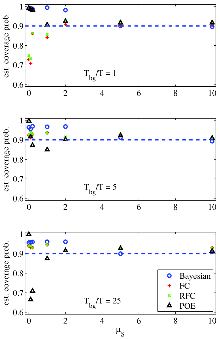
Figure 3: Estimated coverage probabilities for case where $\mu_{B}=1$ for intervals with nominal frequentist coverage probability of 0.90.

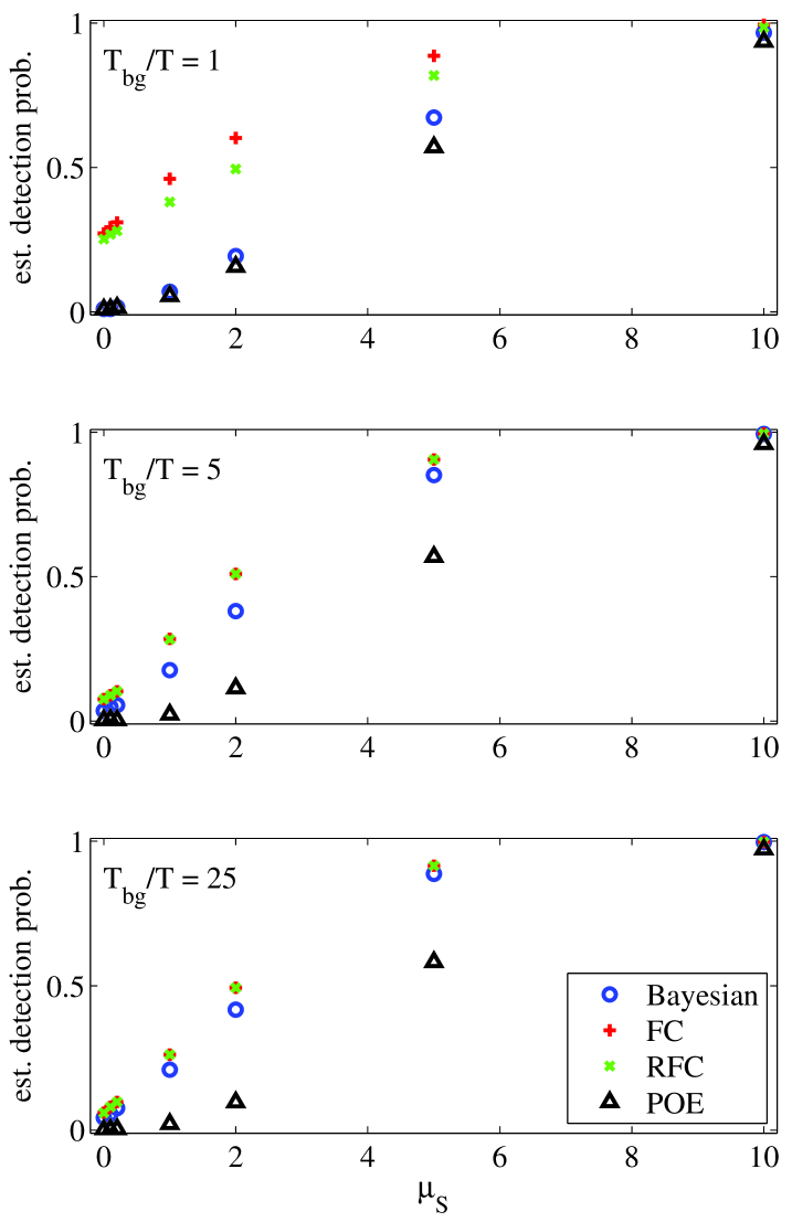
Figure 4: Estimated detection probabilities for case where $\mu_{B}=1$ for intervals with nominal frequentist coverage probability of 0.90.

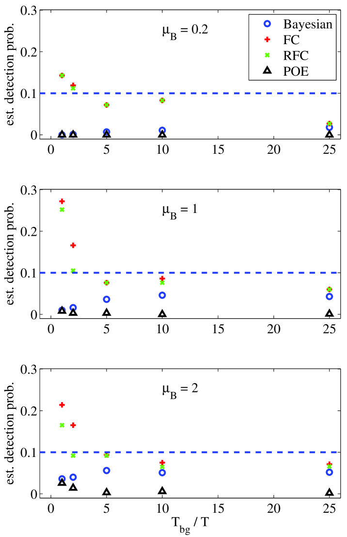
Figure 5: Estimated detection probabilities for case where there is no signal ($\mu_{S}=0$) associated with intervals with nominal frequentist coverage probability of 0.90.

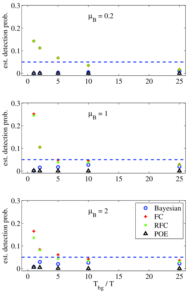
Figure 6: Estimated detection probabilities for case where there is no signal ($\mu_{S}=0$) associated with intervals with nominal frequentist coverage probability of 0.95.

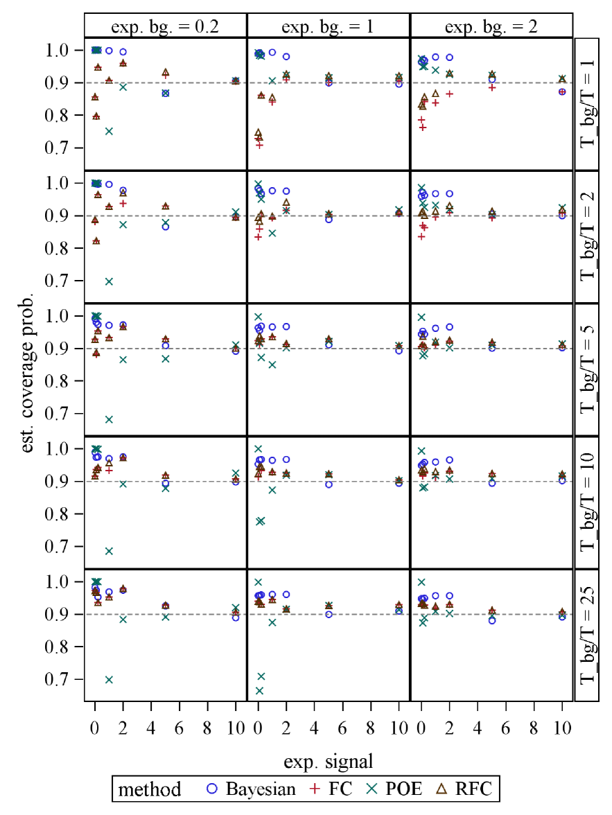
Figure 7: Estimated coverage probabilities corresponding to intervals with target coverage of 0.90. In the plots, we show results for $\mu_{B}=0.2,1,2$ and $T_{bg}/T=1,2,5,10,25$.

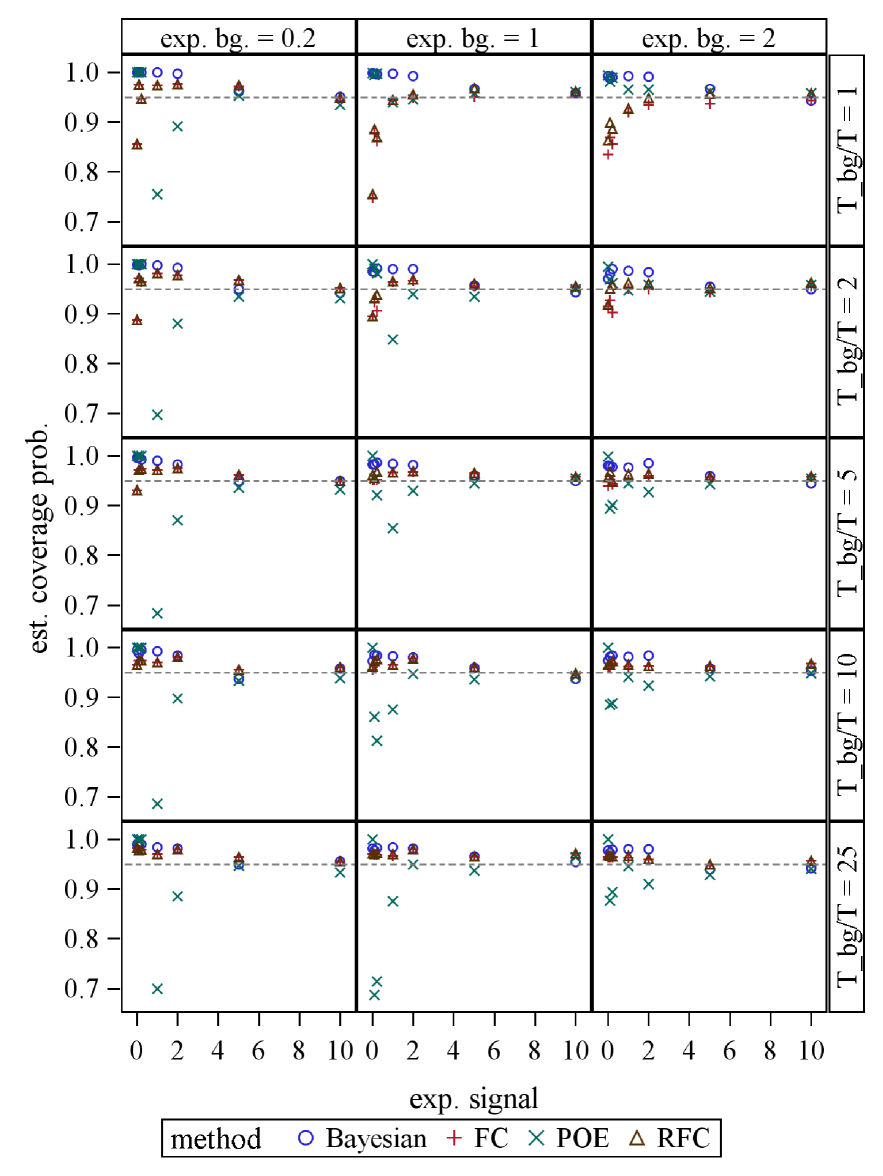
Figure 8: Estimated coverage probabilities corresponding to intervals with target coverage of 0.95. In the plots, we show results for $\mu_{B}=0.2,1,2$ and $T_{bg}/T=1,2,5,10,25$.

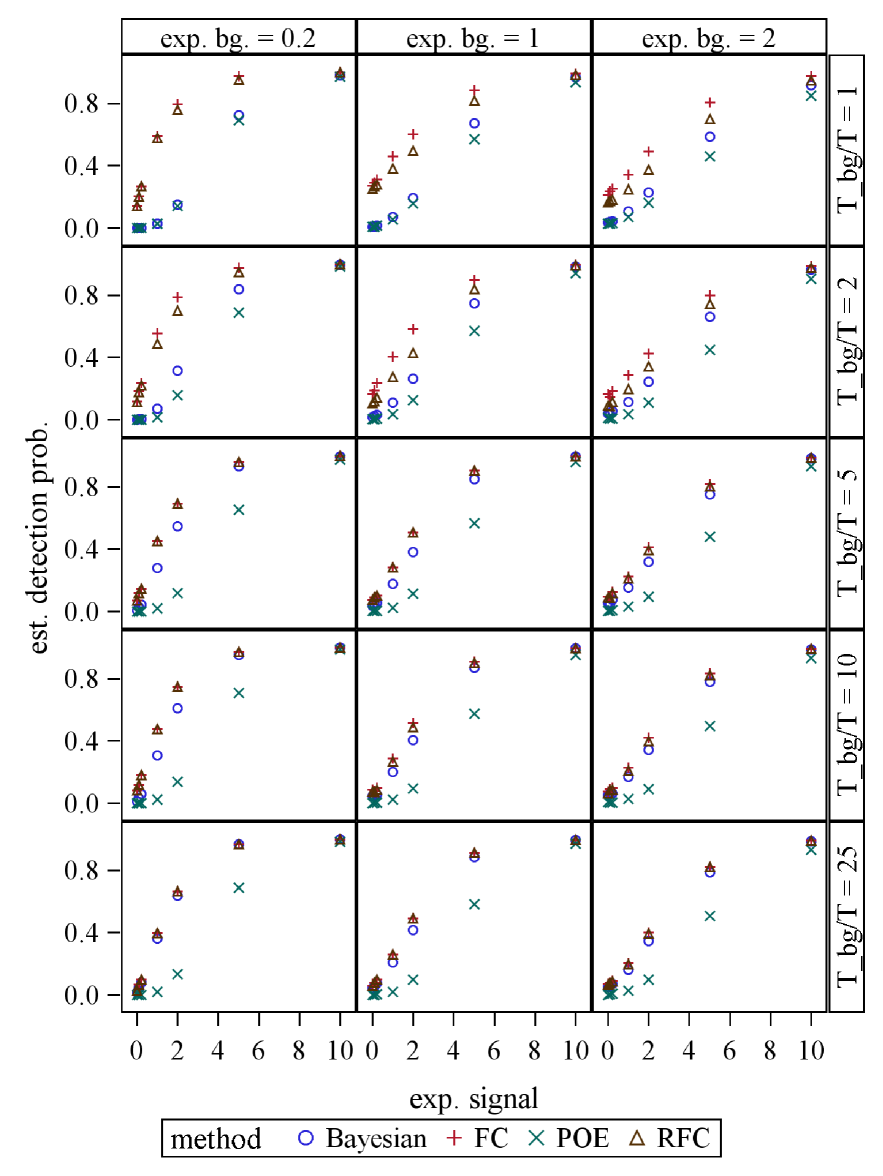
Figure 9: Estimated detection probabilities corresponding to intervals with target coverage of 0.90. In the plots, we show results for $\mu_{B}=0.2,1,2$ and $T_{bg}/T=1,2,5,10,25$.

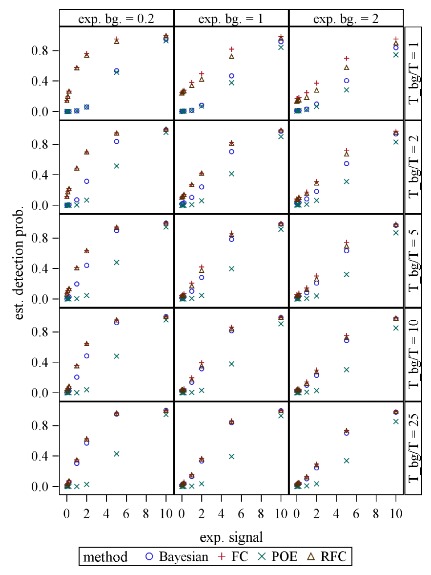
Figure 10: Estimated detection probabilities corresponding to intervals with target coverage of 0.95. In the plots, we show results for $\mu_{B}=0.2,1,2$ and $T_{bg}/T=1,2,5,10,25$.

To start, we consider 90 percent intervals for the case where $\mu_{B}=1$. In Figures 3 and 4, we show coverage and detection probabilities as a function of $\mu_{S}$ and $\frac{T_{bg}}{T}$ for this case. In general, when $\frac{T_{bg}}{T}=1$, the coverage properties of the FC and RFC methods are poor at low value of $\mu_{S}$. In Figures 5 and 6, we show the false detection probabilies for all cases for $\mu_{S}=0$. For $\frac{T_{bg}}{T}=1,2$, both the RFC and FC methods have false detection probabilities that are higher than predicted according to the nominal frequentist coverage of the intervals. Hence, reporting a discovery based on an analysis with the FC or RFC method should be treated with great caution for cases where $\frac{T_{bg}}{T}=1,2$. For $\frac{T_{bg}}{T}\geq 5$, the false detection probabilities of the FC and RFC methods are generally slightly less than their associated nominal target values. In contrast, for all values of $\frac{T_{bg}}{T}$, the false detection probabilities of the Bayesian method are less than the values predicted by the nominal frequentist coverage. In Figures 7-10, we display coverage and detection probabilities for all cases considered in our simulation study.

In Tables 14 and 15, we list the root-mean-square (RMS) deviation between the observed and nominal frequentist coverage probabilities as a function of $\mu_{B}$. We include results for $\mu_{S}\leq 10$. According to our coverage and detection probability criteria, the POE method performed the least well of all methods. This is not a surprise since the poor performance of the POE method for low-count situations is well known. In general, the Bayesian method yielded intervals with the lowest detection probabilities compared to the FC and RFC methods. According to the RMS coverage criterion, the coverage properties of the Bayesian intervals are inferior to the intervals produces by the FC and RFC methods for most cases. The exception to this pattern was for the case where $\frac{T_{bg}}{T}=1$ and $\mu_{B}=1,2$. The FC and RFC method had better coverage compared to Bayesian method for $\mu_{B}=0.2$ for all values of $\frac{T_{bg}}{T}$ considered.

For $\frac{T_{bg}}{T}=1,2$ the coverage properties of the RFC method where slightly better than those of the FC method for $\mu_{B}=1,2$. However, for $\frac{T_{bg}}{T}$ greater than or equal to 5, the FC method yields intervals with superior coverage and detection probabilities compared to the RFC and Bayesian methods.

3.1 Comments

For fixed $\mu_{B}$, as $\mu_{S}$ increases, we sometimes observe nonmonotic trends in coverage. In other studies such as [24], nonmonotic trends were also observed.

We expect the FC method to yield poor results when the 1-sigma uncertainty in the estimated background (Eq. 5) is large. For $\frac{T_{bg}}{T}=$ 1 and $\mu_{B}=$ 0.2, 1, 2, Eq. 5 yields absolute uncertainties of 0.45, 1 and 1.41, and Eq. 6 yields fractional uncertainties of 224 $\%$, 100 $\%$ and 71 $\%$ respectively. For $\frac{T_{bg}}{T}=$ 5, the absolute and fractional uncertainties are 0.2, 0.45 and 0.63, and 100 $\%$, 45 $\%$ and 31 $\%$ respectively. For $\frac{T_{bg}}{T}=$ 25, the absolute and fractional uncertainties are 0.09, 0.20 and 0.28, and 45 $\%$, 20 $\%$ and 14 $\%$ respectively.

It is plausible that the performance of the FC method depends solely on the Eq. 5 uncertainty of the background estimate. However, comparison of the coverage properties of the FC intervals for the case where $\frac{T_{bg}}{T}=$ 1, $\mu_{B}=0.2$ and for the case where $\frac{T_{bg}}{T}=$ 5, $\mu_{B}=1$, suggest a more complicated picture. For the first case, the FC intervals have poor coverage at low values of $\mu_{S}$ (Tables 2,5). For the second case, the intervals have good coverage at all $\mu_{S}$ (Tables 3,6). However, the standard deviation of the estimated background is the same for both cases. Perhaps this result is due to differences in the shapes of the background estimate pdfs for $\frac{T_{bg}}{T}=1$ and $\frac{T_{bg}}{T}=5$.

In the POE method, we approximate the distribution of the background-corrected estimate of $\mu_{S}$, $n_{obs}-\hat{\mu}_{B}$, as a normal (Gaussian) random variable. For the special case where $\mu_{B}=$ 0, a common rule of thumb is that the normal approximation is reasonable when the expected value of $n_{obs}$ is greater than about 10 [27]. From this, we conclude that if the expected values of of $n_{obs}$ and $n_{bg}$ both exceed 10, the Gaussian assumption seems reasonable. As a caveat, the adequacy of the normal approximation depends on the goal of the analysis. For instance, constructing a confidence interval with nominal coverage of 0.99 is a more demanding task than constructing an interval with nominal coverage of 0.90. For the cases studied here where the nominal coverage is 0.90 or 0.95, the POE intervals had coverage close to the desired nominal values when $\mu_{S}$ was greater than about 5.

In our implementation of the Bayesian method, we specify uniform priors for $\mu_{S}$ and $\mu_{B}$ and construct a minimum length credibility interval. Roe and Woodroofe [24] determined a minimum length credibility interval based on a uniform prior for $\mu_{S}$ for the simpler problem where $\mu_{B}$ was assumed to be known. Hence, our study can be regarded a generalization of [24] to the case where $\mu_{B}$ is not known exactly. As a caveat, in a Bayesian approach, one could consider other priors. For a given experiment, it is possible that other priors might be more appropriate than the uniform prior considered here. How well such alternative Bayesian schemes would perform relative to the one studied here is beyond the scope of this study.

As remarked earlier, we did not adjust our intervals to ensure that the upper endpoint of the FC and RFC intervals are nondecreasing functions of $\mu_{B}$. It is possible that such an adjustment might improve the performance of the FC and RFC methods. Also, the FC method of computing the likelihood-ratio term $R$ may not be the best procedure [28-31].

4 Summary

In this work, we studied four methods to construct uncertainty intervals for very weak Poisson signals in the presence of background. We considered the case where a primary experiment yielded a realization of the signal plus background, and a second experiment yielded a realization of the background. The duration of the background-only experiment $T_{bg}$ and and the duration of the primary experiment $T$ were selected so that $\frac{T_{bg}}{T}$ varied from 1 to 25. This choice of $\frac{T_{bg}}{T}=$25 was motivated by experimental studies at NIST. The values of the expected background $\mu_{B}$ varied from 0.2 to 2. The choice of the range was also motivated by NIST experiments.

We constructed confidence intervals based on the standard propagation-of-errors method as well as two implementations of a Neyman procedure due to Feldman and Cousins (FC) and Conrad (RFC). In the FC method, uncertainty in the background was neglected. In our implementation of the RFC method, uncertainty in the background parameter was accounted for. In both of these methods, acceptance regions were determined for each value of the expected signal rate based on a likelihood-ratio ordering principle. Hence, the upper and lower endpoints of the confidence intervals were automatically selected. We also constructed minimum length Bayesian credibility intervals.

According to our coverage and detection probability criteria, the POE method performed the least well of all methods. In general, the Bayesian method yielded intervals with the lowest detection probabilities compared to the FC and RFC methods (Tables 8-13, Figures 4,5,6,8 and 10). According to an RMS criterion, the coverage properties of the Bayesian intervals were inferior to the intervals produces by the FC and RFC methods (Tables 14 and 15) for most cases. The exception to this pattern was for the case where $\frac{T_{bg}}{T}=1$ and $\mu_{B}=1,2$.

The FC and RFC methods had better coverage compared to the Bayesian method for $\mu_{B}=0.2$ for all values of $\frac{T_{bg}}{T}$ considered. We expect similar results for $\mu_{B}<0.2$. We interpret this result as evidence that when expected number of background counts is 0.2 or less, the FC method (which neglects uncertainty in the background) works well because uncertainty in the observed background is not significant compared to other sources of uncertainty that affect the interval.

For $\frac{T_{bg}}{T}=1,2$ the coverage properties of the RFC method where slightly better than those of the FC method for $\mu_{B}=1,2$. However, for $\frac{T_{bg}}{T}$ greater than or equal to 5, the FC method yielded intervals with superior coverage and detection probabilities compared to the RFC and Bayesian methods. We attribute the good performance of the FC method to the fact that uncertainty in the estimated background is not significant compared to other sources of uncertainty that affect the interval when $\mu_{B}\leq 2$ and $\frac{T_{bg}}{T}\geq 5$. The relative performance of the three methods for $\mu_{B}>2$ is an open question. We speculate that for the FC method to yield a result superior to the Bayesian or RFC method for $\mu_{B}$ much larger than 2, $\frac{T_{bg}}{T}$ may have to be larger than 5 in order to reduce the uncertainty of estimated background to a sufficiently low level.

As a caveat, for $\frac{T_{bg}}{T}=1,2$, both the RFC and FC methods had false detection probabilities that were higher than predicted according to the nominal frequentist coverage of the intervals for $\frac{T_{bg}}{T}=1,2$ (Figures 5,6). Hence, reporting a discovery based on an analysis with the FC or RFC method should be treated with great caution for cases where $\frac{T_{bg}}{T}=1,2$. For $\frac{T_{bg}}{T}\geq 5$, the false detection probabilities of the FC and RFC methods were generally slightly less than their associated nominal target values. In contrast, for all values of $\frac{T_{bg}}{T}$, the false detection probabilities of the Bayesian method were less than the value predicted by the nominal frequentist coverage.

Acknowledgements

We thank H.K. Liu, L.A. Currie and the anonymous reviewers of this work for useful comments.

Table 1. Upper and lower endpoints of uncertainty intervals with nominal frequentist coverage of 0.90. The intervals are determined from simulated values of $n_{obs}$ and $n_{bg}$. For informational purposes, we list $\mu_{S}$ and $\mu_{B}$.
Bayesian Bayesian FC FC RFC RFC POE POE $\frac{T_{bg}}{T}$ $\mu_{S}$ $\mu_{B}$ $n_{obs}$ $n_{bg}$ Lower Upper Lower Upper Lower Upper Lower Upper 1 1.0 2.0 2 1 0.00 4.32 0.00 4.91 0.00 5.27 -2.35 4.35 1 10.0 0.2 6 0 1.58 10.42 2.21 11.46 2.21 11.46 1.47 10.53 5 2.0 0.2 1 0 0.00 3.74 0.11 4.35 0.11 4.35 -1.14 3.14 5 1.0 1.0 1 4 0.00 3.34 0.00 3.55 0.00 3.56 -2.07 2.47 5 5.0 2.0 5 7 0.49 8.11 1.04 8.58 0.95 8.58 -0.68 7.88 25 0.1 2.0 0 46 0.00 2.30 0.00 1.15 0.00 1.15 -2.79 -0.89 25 5.0 1.0 2 16 0.00 4.70 0.00 5.27 0.00 5.27 -1.48 4.20 25 10.0 0.2 9 7 4.57 14.62 4.08 15.01 4.08 15.04 3.28 14.16

Table 2. Estimated coverage probabilities of uncertainty intervals with nominal frequentist coverage of 0.90. Approximate 68 percent uncertainty due to sampling variability given for cases where estimated coverage probability is greater than 0 or less than 1. $\frac{T_{bg}}{T}=1$.
$\mu_{S}$ $\mu_{B}$ Bayesian FC RFC POE 0.0 0.2 1 0.857$\pm$ 0.008 0.857$\pm$ 0.008 1 0.1 0.2 1 0.797$\pm$ 0.009 0.798$\pm$ 0.009 1 0.2 0.2 1 0.948$\pm$ 0.005 0.948$\pm$ 0.005 1 1.0 0.2 0.998$\pm$ 0.001 0.908$\pm$ 0.006 0.908$\pm$ 0.006 0.751$\pm$ 0.010 2.0 0.2 0.995$\pm$ 0.002 0.960$\pm$ 0.004 0.961$\pm$ 0.004 0.887$\pm$ 0.007 5.0 0.2 0.867$\pm$ 0.008 0.923$\pm$ 0.006 0.933$\pm$ 0.006 0.869$\pm$ 0.008 10.0 0.2 0.906$\pm$ 0.007 0.904$\pm$ 0.007 0.906$\pm$ 0.007 0.907$\pm$ 0.007 20.0 0.2 0.911$\pm$ 0.006 0.904$\pm$ 0.007 0.908$\pm$ 0.006 0.911$\pm$ 0.006 0.0 1.0 0.990$\pm$ 0.002 0.728$\pm$ 0.010 0.748$\pm$ 0.010 0.991$\pm$ 0.002 0.1 1.0 0.992$\pm$ 0.002 0.708$\pm$ 0.010 0.733$\pm$ 0.010 0.985$\pm$ 0.003 0.2 1.0 0.986$\pm$ 0.003 0.861$\pm$ 0.008 0.862$\pm$ 0.008 0.982$\pm$ 0.003 1.0 1.0 0.994$\pm$ 0.002 0.841$\pm$ 0.008 0.856$\pm$ 0.008 0.906$\pm$ 0.007 2.0 1.0 0.981$\pm$ 0.003 0.909$\pm$ 0.006 0.927$\pm$ 0.006 0.924$\pm$ 0.006 5.0 1.0 0.900$\pm$ 0.007 0.901$\pm$ 0.007 0.922$\pm$ 0.006 0.916$\pm$ 0.006 10.0 1.0 0.896$\pm$ 0.007 0.906$\pm$ 0.007 0.921$\pm$ 0.006 0.917$\pm$ 0.006 20.0 1.0 0.903$\pm$ 0.007 0.886$\pm$ 0.007 0.901$\pm$ 0.007 0.903$\pm$ 0.007 0.0 2.0 0.964$\pm$ 0.004 0.786$\pm$ 0.009 0.835$\pm$ 0.008 0.974$\pm$ 0.004 0.1 2.0 0.972$\pm$ 0.004 0.763$\pm$ 0.010 0.828$\pm$ 0.008 0.949$\pm$ 0.005 0.2 2.0 0.968$\pm$ 0.004 0.843$\pm$ 0.008 0.857$\pm$ 0.008 0.951$\pm$ 0.005 1.0 2.0 0.980$\pm$ 0.003 0.838$\pm$ 0.008 0.867$\pm$ 0.008 0.939$\pm$ 0.005 2.0 2.0 0.978$\pm$ 0.003 0.866$\pm$ 0.008 0.930$\pm$ 0.006 0.926$\pm$ 0.006 5.0 2.0 0.910$\pm$ 0.006 0.886$\pm$ 0.007 0.927$\pm$ 0.006 0.924$\pm$ 0.006 10.0 2.0 0.872$\pm$ 0.007 0.872$\pm$ 0.007 0.912$\pm$ 0.006 0.913$\pm$ 0.006 20.0 2.0 0.907$\pm$ 0.007 0.886$\pm$ 0.007 0.908$\pm$ 0.006 0.910$\pm$ 0.006

Table 3. Estimated coverage probabilities of uncertainty intervals with nominal frequentist coverage of 0.90. Approximate 68 percent uncertainty due to sampling variability given for cases where estimated coverage probability is greater than 0 or less than 1. $\frac{T_{bg}}{T}=5$.
$\mu_{S}$ $\mu_{B}$ Bayesian FC RFC POE 0.0 0.2 0.993$\pm$ 0.002 0.928$\pm$ 0.006 0.928$\pm$ 0.006 1 0.1 0.2 0.981$\pm$ 0.003 0.882$\pm$ 0.007 0.888$\pm$ 0.007 1 0.2 0.2 0.974$\pm$ 0.004 0.955$\pm$ 0.005 0.955$\pm$ 0.005 0.999$\pm$ 0.001 1.0 0.2 0.971$\pm$ 0.004 0.934$\pm$ 0.006 0.934$\pm$ 0.006 0.682$\pm$ 0.010 2.0 0.2 0.973$\pm$ 0.004 0.967$\pm$ 0.004 0.967$\pm$ 0.004 0.866$\pm$ 0.008 5.0 0.2 0.909$\pm$ 0.006 0.930$\pm$ 0.006 0.930$\pm$ 0.006 0.868$\pm$ 0.008 10.0 0.2 0.892$\pm$ 0.007 0.901$\pm$ 0.007 0.901$\pm$ 0.007 0.912$\pm$ 0.006 20.0 0.2 0.892$\pm$ 0.007 0.894$\pm$ 0.007 0.894$\pm$ 0.007 0.907$\pm$ 0.006 0.0 1.0 0.964$\pm$ 0.004 0.924$\pm$ 0.006 0.924$\pm$ 0.006 0.997$\pm$ 0.001 0.1 1.0 0.956$\pm$ 0.005 0.911$\pm$ 0.006 0.939$\pm$ 0.005 0.916$\pm$ 0.006 0.2 1.0 0.969$\pm$ 0.004 0.929$\pm$ 0.006 0.929$\pm$ 0.006 0.872$\pm$ 0.007 1.0 1.0 0.967$\pm$ 0.004 0.936$\pm$ 0.005 0.937$\pm$ 0.005 0.850$\pm$ 0.008 2.0 1.0 0.968$\pm$ 0.004 0.912$\pm$ 0.006 0.915$\pm$ 0.006 0.902$\pm$ 0.007 5.0 1.0 0.912$\pm$ 0.006 0.929$\pm$ 0.006 0.929$\pm$ 0.006 0.922$\pm$ 0.006 10.0 1.0 0.893$\pm$ 0.007 0.909$\pm$ 0.006 0.909$\pm$ 0.006 0.909$\pm$ 0.006 20.0 1.0 0.891$\pm$ 0.007 0.897$\pm$ 0.007 0.902$\pm$ 0.007 0.901$\pm$ 0.007 0.0 2.0 0.944$\pm$ 0.005 0.906$\pm$ 0.007 0.908$\pm$ 0.006 0.996$\pm$ 0.001 0.1 2.0 0.954$\pm$ 0.005 0.912$\pm$ 0.006 0.938$\pm$ 0.005 0.877$\pm$ 0.007 0.2 2.0 0.944$\pm$ 0.005 0.902$\pm$ 0.007 0.907$\pm$ 0.006 0.884$\pm$ 0.007 1.0 2.0 0.963$\pm$ 0.004 0.910$\pm$ 0.006 0.922$\pm$ 0.006 0.920$\pm$ 0.006 2.0 2.0 0.966$\pm$ 0.004 0.921$\pm$ 0.006 0.926$\pm$ 0.006 0.902$\pm$ 0.007 5.0 2.0 0.901$\pm$ 0.007 0.919$\pm$ 0.006 0.920$\pm$ 0.006 0.910$\pm$ 0.006 10.0 2.0 0.902$\pm$ 0.007 0.909$\pm$ 0.006 0.913$\pm$ 0.006 0.914$\pm$ 0.006 20.0 2.0 0.897$\pm$ 0.007 0.902$\pm$ 0.007 0.905$\pm$ 0.007 0.908$\pm$ 0.006

Table 4. Estimated coverage probabilities of uncertainty intervals with nominal frequentist coverage of 0.90. Approximate 68 percent uncertainty due to sampling variability given for cases where estimated coverage probability is greater than 0 or less than 1. $\frac{T_{bg}}{T}=25$.
$\mu_{S}$ $\mu_{B}$ Bayesian FC RFC POE 0.0 0.2 0.982$\pm$ 0.003 0.973$\pm$ 0.004 0.973$\pm$ 0.004 1 0.1 0.2 0.974$\pm$ 0.004 0.967$\pm$ 0.004 0.967$\pm$ 0.004 1 0.2 0.2 0.953$\pm$ 0.005 0.937$\pm$ 0.005 0.937$\pm$ 0.005 1 1.0 0.2 0.969$\pm$ 0.004 0.954$\pm$ 0.005 0.954$\pm$ 0.005 0.698$\pm$ 0.010 2.0 0.2 0.974$\pm$ 0.004 0.979$\pm$ 0.003 0.979$\pm$ 0.003 0.884$\pm$ 0.007 5.0 0.2 0.925$\pm$ 0.006 0.928$\pm$ 0.006 0.928$\pm$ 0.006 0.891$\pm$ 0.007 10.0 0.2 0.890$\pm$ 0.007 0.906$\pm$ 0.007 0.906$\pm$ 0.007 0.920$\pm$ 0.006 20.0 0.2 0.906$\pm$ 0.007 0.909$\pm$ 0.006 0.909$\pm$ 0.006 0.920$\pm$ 0.006 0.0 1.0 0.957$\pm$ 0.005 0.940$\pm$ 0.005 0.940$\pm$ 0.005 0.999$\pm$ 0.001 0.1 1.0 0.958$\pm$ 0.005 0.931$\pm$ 0.006 0.939$\pm$ 0.005 0.665$\pm$ 0.011 0.2 1.0 0.960$\pm$ 0.004 0.931$\pm$ 0.006 0.931$\pm$ 0.006 0.709$\pm$ 0.010 1.0 1.0 0.961$\pm$ 0.004 0.946$\pm$ 0.005 0.946$\pm$ 0.005 0.875$\pm$ 0.007 2.0 1.0 0.961$\pm$ 0.004 0.917$\pm$ 0.006 0.917$\pm$ 0.006 0.916$\pm$ 0.006 5.0 1.0 0.900$\pm$ 0.007 0.927$\pm$ 0.006 0.927$\pm$ 0.006 0.927$\pm$ 0.006 10.0 1.0 0.910$\pm$ 0.006 0.930$\pm$ 0.006 0.930$\pm$ 0.006 0.914$\pm$ 0.006 20.0 1.0 0.907$\pm$ 0.006 0.914$\pm$ 0.006 0.914$\pm$ 0.006 0.918$\pm$ 0.006 0.0 2.0 0.948$\pm$ 0.005 0.929$\pm$ 0.006 0.934$\pm$ 0.006 0.998$\pm$ 0.001 0.1 2.0 0.946$\pm$ 0.005 0.930$\pm$ 0.006 0.933$\pm$ 0.006 0.873$\pm$ 0.007 0.2 2.0 0.949$\pm$ 0.005 0.928$\pm$ 0.006 0.928$\pm$ 0.006 0.889$\pm$ 0.007 1.0 2.0 0.957$\pm$ 0.005 0.919$\pm$ 0.006 0.924$\pm$ 0.006 0.909$\pm$ 0.006 2.0 2.0 0.957$\pm$ 0.005 0.930$\pm$ 0.006 0.931$\pm$ 0.006 0.902$\pm$ 0.007 5.0 2.0 0.881$\pm$ 0.007 0.913$\pm$ 0.006 0.913$\pm$ 0.006 0.896$\pm$ 0.007 10.0 2.0 0.892$\pm$ 0.007 0.908$\pm$ 0.006 0.909$\pm$ 0.006 0.897$\pm$ 0.007 20.0 2.0 0.900$\pm$ 0.007 0.909$\pm$ 0.006 0.909$\pm$ 0.006 0.912$\pm$ 0.006

Table 5. Estimated coverage probabilities of uncertainty intervals with nominal frequentist coverage of 0.95. Approximate 68 percent uncertainty due to sampling variability given for cases where estimated coverage probability is greater than 0 or less than 1. $\frac{T_{bg}}{T}=1$.
$\mu_{S}$ $\mu_{B}$ Bayesian FC RFC POE 0.0 0.2 1 0.857$\pm$ 0.008 0.857$\pm$ 0.008 1 0.1 0.2 1 0.976$\pm$ 0.003 0.976$\pm$ 0.003 1 0.2 0.2 1 0.948$\pm$ 0.005 0.948$\pm$ 0.005 1 1.0 0.2 1 0.974$\pm$ 0.004 0.974$\pm$ 0.004 0.755$\pm$ 0.010 2.0 0.2 0.998$\pm$ 0.001 0.976$\pm$ 0.003 0.977$\pm$ 0.003 0.892$\pm$ 0.007 5.0 0.2 0.962$\pm$ 0.004 0.972$\pm$ 0.004 0.974$\pm$ 0.004 0.953$\pm$ 0.005 10.0 0.2 0.951$\pm$ 0.005 0.949$\pm$ 0.005 0.949$\pm$ 0.005 0.935$\pm$ 0.006 20.0 0.2 0.949$\pm$ 0.005 0.953$\pm$ 0.005 0.955$\pm$ 0.005 0.950$\pm$ 0.005 0.0 1.0 0.999$\pm$ 0.001 0.748$\pm$ 0.010 0.755$\pm$ 0.010 0.999$\pm$ 0.001 0.1 1.0 0.998$\pm$ 0.001 0.878$\pm$ 0.007 0.886$\pm$ 0.007 0.995$\pm$ 0.002 0.2 1.0 0.997$\pm$ 0.001 0.862$\pm$ 0.008 0.870$\pm$ 0.008 0.998$\pm$ 0.001 1.0 1.0 0.998$\pm$ 0.001 0.945$\pm$ 0.005 0.945$\pm$ 0.005 0.940$\pm$ 0.005 2.0 1.0 0.993$\pm$ 0.002 0.949$\pm$ 0.005 0.956$\pm$ 0.005 0.946$\pm$ 0.005 5.0 1.0 0.967$\pm$ 0.004 0.951$\pm$ 0.005 0.969$\pm$ 0.004 0.958$\pm$ 0.004 10.0 1.0 0.958$\pm$ 0.004 0.959$\pm$ 0.004 0.962$\pm$ 0.004 0.960$\pm$ 0.004 20.0 1.0 0.954$\pm$ 0.005 0.944$\pm$ 0.005 0.955$\pm$ 0.005 0.950$\pm$ 0.005 0.0 2.0 0.993$\pm$ 0.002 0.835$\pm$ 0.008 0.864$\pm$ 0.008 0.994$\pm$ 0.002 0.1 2.0 0.988$\pm$ 0.002 0.869$\pm$ 0.008 0.900$\pm$ 0.007 0.981$\pm$ 0.003 0.2 2.0 0.990$\pm$ 0.002 0.856$\pm$ 0.008 0.887$\pm$ 0.007 0.989$\pm$ 0.002 1.0 2.0 0.993$\pm$ 0.002 0.921$\pm$ 0.006 0.928$\pm$ 0.006 0.965$\pm$ 0.004 2.0 2.0 0.991$\pm$ 0.002 0.935$\pm$ 0.006 0.948$\pm$ 0.005 0.966$\pm$ 0.004 5.0 2.0 0.967$\pm$ 0.004 0.937$\pm$ 0.005 0.957$\pm$ 0.005 0.962$\pm$ 0.004 10.0 2.0 0.944$\pm$ 0.005 0.943$\pm$ 0.005 0.958$\pm$ 0.004 0.958$\pm$ 0.004 20.0 2.0 0.952$\pm$ 0.005 0.945$\pm$ 0.005 0.957$\pm$ 0.005 0.958$\pm$ 0.005

Table 6. Estimated coverage probabilities of uncertainty intervals with nominal frequentist coverage of 0.95. Approximate 68 percent uncertainty due to sampling variability given for cases where estimated coverage probability is greater than 0 or less than 1. $\frac{T_{bg}}{T}=5$.
$\mu_{S}$ $\mu_{B}$ Bayesian FC RFC POE 0.0 0.2 0.997$\pm$ 0.001 0.932$\pm$ 0.006 0.932$\pm$ 0.006 1 0.1 0.2 0.997$\pm$ 0.001 0.972$\pm$ 0.004 0.972$\pm$ 0.004 1 0.2 0.2 0.993$\pm$ 0.002 0.974$\pm$ 0.004 0.974$\pm$ 0.004 1 1.0 0.2 0.990$\pm$ 0.002 0.971$\pm$ 0.004 0.971$\pm$ 0.004 0.684$\pm$ 0.010 2.0 0.2 0.983$\pm$ 0.003 0.976$\pm$ 0.003 0.976$\pm$ 0.003 0.871$\pm$ 0.007 5.0 0.2 0.950$\pm$ 0.005 0.962$\pm$ 0.004 0.962$\pm$ 0.004 0.936$\pm$ 0.005 10.0 0.2 0.949$\pm$ 0.005 0.950$\pm$ 0.005 0.950$\pm$ 0.005 0.933$\pm$ 0.006 20.0 0.2 0.945$\pm$ 0.005 0.951$\pm$ 0.005 0.955$\pm$ 0.005 0.950$\pm$ 0.005 0.0 1.0 0.983$\pm$ 0.003 0.952$\pm$ 0.005 0.962$\pm$ 0.004 1 0.1 1.0 0.983$\pm$ 0.003 0.953$\pm$ 0.005 0.955$\pm$ 0.005 0.955$\pm$ 0.005 0.2 1.0 0.986$\pm$ 0.003 0.953$\pm$ 0.005 0.969$\pm$ 0.004 0.921$\pm$ 0.006 1.0 1.0 0.984$\pm$ 0.003 0.967$\pm$ 0.004 0.967$\pm$ 0.004 0.855$\pm$ 0.008 2.0 1.0 0.982$\pm$ 0.003 0.968$\pm$ 0.004 0.969$\pm$ 0.004 0.930$\pm$ 0.006 5.0 1.0 0.961$\pm$ 0.004 0.966$\pm$ 0.004 0.966$\pm$ 0.004 0.945$\pm$ 0.005 10.0 1.0 0.950$\pm$ 0.005 0.959$\pm$ 0.004 0.959$\pm$ 0.004 0.955$\pm$ 0.005 20.0 1.0 0.946$\pm$ 0.005 0.946$\pm$ 0.005 0.950$\pm$ 0.005 0.941$\pm$ 0.005 0.0 2.0 0.980$\pm$ 0.003 0.939$\pm$ 0.005 0.957$\pm$ 0.005 0.999$\pm$ 0.001 0.1 2.0 0.980$\pm$ 0.003 0.954$\pm$ 0.005 0.969$\pm$ 0.004 0.895$\pm$ 0.007 0.2 2.0 0.978$\pm$ 0.003 0.943$\pm$ 0.005 0.948$\pm$ 0.005 0.902$\pm$ 0.007 1.0 2.0 0.977$\pm$ 0.003 0.951$\pm$ 0.005 0.963$\pm$ 0.004 0.945$\pm$ 0.005 2.0 2.0 0.985$\pm$ 0.003 0.959$\pm$ 0.004 0.965$\pm$ 0.004 0.927$\pm$ 0.006 5.0 2.0 0.960$\pm$ 0.004 0.957$\pm$ 0.005 0.958$\pm$ 0.005 0.943$\pm$ 0.005 10.0 2.0 0.945$\pm$ 0.005 0.959$\pm$ 0.004 0.959$\pm$ 0.004 0.954$\pm$ 0.005 20.0 2.0 0.944$\pm$ 0.005 0.947$\pm$ 0.005 0.949$\pm$ 0.005 0.947$\pm$ 0.005

Table 7. Estimated coverage probabilities of uncertainty intervals with nominal frequentist coverage of 0.95. Approximate 68 percent uncertainty due to sampling variability given for cases where estimated coverage probability is greater than 0 or less than 1. $\frac{T_{bg}}{T}=25$.
$\mu_{S}$ $\mu_{B}$ Bayesian FC RFC POE 0.0 0.2 0.990$\pm$ 0.002 0.983$\pm$ 0.003 0.983$\pm$ 0.003 1 0.1 0.2 0.987$\pm$ 0.003 0.978$\pm$ 0.003 0.978$\pm$ 0.003 1 0.2 0.2 0.990$\pm$ 0.002 0.979$\pm$ 0.003 0.979$\pm$ 0.003 1 1.0 0.2 0.984$\pm$ 0.003 0.970$\pm$ 0.004 0.970$\pm$ 0.004 0.700$\pm$ 0.010 2.0 0.2 0.982$\pm$ 0.003 0.981$\pm$ 0.003 0.981$\pm$ 0.003 0.886$\pm$ 0.007 5.0 0.2 0.949$\pm$ 0.005 0.964$\pm$ 0.004 0.964$\pm$ 0.004 0.948$\pm$ 0.005 10.0 0.2 0.956$\pm$ 0.005 0.956$\pm$ 0.005 0.956$\pm$ 0.005 0.934$\pm$ 0.006 20.0 0.2 0.948$\pm$ 0.005 0.956$\pm$ 0.005 0.956$\pm$ 0.005 0.958$\pm$ 0.005 0.0 1.0 0.981$\pm$ 0.003 0.971$\pm$ 0.004 0.972$\pm$ 0.004 1 0.1 1.0 0.978$\pm$ 0.003 0.970$\pm$ 0.004 0.970$\pm$ 0.004 0.687$\pm$ 0.010 0.2 1.0 0.983$\pm$ 0.003 0.969$\pm$ 0.004 0.973$\pm$ 0.004 0.715$\pm$ 0.010 1.0 1.0 0.984$\pm$ 0.003 0.967$\pm$ 0.004 0.970$\pm$ 0.004 0.876$\pm$ 0.007 2.0 1.0 0.981$\pm$ 0.003 0.980$\pm$ 0.003 0.980$\pm$ 0.003 0.949$\pm$ 0.005 5.0 1.0 0.966$\pm$ 0.004 0.966$\pm$ 0.004 0.966$\pm$ 0.004 0.937$\pm$ 0.005 10.0 1.0 0.955$\pm$ 0.005 0.972$\pm$ 0.004 0.972$\pm$ 0.004 0.965$\pm$ 0.004 20.0 1.0 0.956$\pm$ 0.005 0.956$\pm$ 0.005 0.956$\pm$ 0.005 0.954$\pm$ 0.005 0.0 2.0 0.978$\pm$ 0.003 0.964$\pm$ 0.004 0.969$\pm$ 0.004 1 0.1 2.0 0.973$\pm$ 0.004 0.964$\pm$ 0.004 0.967$\pm$ 0.004 0.877$\pm$ 0.007 0.2 2.0 0.979$\pm$ 0.003 0.964$\pm$ 0.004 0.966$\pm$ 0.004 0.894$\pm$ 0.007 1.0 2.0 0.981$\pm$ 0.003 0.964$\pm$ 0.004 0.967$\pm$ 0.004 0.946$\pm$ 0.005 2.0 2.0 0.981$\pm$ 0.003 0.960$\pm$ 0.004 0.961$\pm$ 0.004 0.911$\pm$ 0.006 5.0 2.0 0.940$\pm$ 0.005 0.950$\pm$ 0.005 0.949$\pm$ 0.005 0.929$\pm$ 0.006 10.0 2.0 0.942$\pm$ 0.005 0.957$\pm$ 0.005 0.957$\pm$ 0.005 0.941$\pm$ 0.005 20.0 2.0 0.946$\pm$ 0.005 0.952$\pm$ 0.005 0.952$\pm$ 0.005 0.948$\pm$ 0.005

Table 8. Estimated detection probabilities corresponding to uncertainty intervals with nominal frequentist coverage of 0.90. Approximate 68 percent uncertainty due to sampling variability given for cases where estimated coverage probability is greater than 0 or less than 1. $\frac{T_{bg}}{T}=1$.
$\mu_{S}$ $\mu_{B}$ Bayesian FC RFC POE 0.0 0.2 0 0.143$\pm$ 0.008 0.143$\pm$ 0.008 0 0.1 0.2 0 0.203$\pm$ 0.009 0.202$\pm$ 0.009 0 0.2 0.2 0.001$\pm$ 0.001 0.269$\pm$ 0.010 0.268$\pm$ 0.010 0.001$\pm$ 0.001 1.0 0.2 0.028$\pm$ 0.004 0.591$\pm$ 0.011 0.580$\pm$ 0.011 0.027$\pm$ 0.004 2.0 0.2 0.152$\pm$ 0.008 0.795$\pm$ 0.009 0.759$\pm$ 0.010 0.144$\pm$ 0.008 5.0 0.2 0.725$\pm$ 0.010 0.975$\pm$ 0.004 0.951$\pm$ 0.005 0.695$\pm$ 0.010 10.0 0.2 0.979$\pm$ 0.003 1 0.998$\pm$ 0.001 0.971$\pm$ 0.004 20.0 0.2 1 1 1 1 0.0 1.0 0.010$\pm$ 0.002 0.272$\pm$ 0.010 0.252$\pm$ 0.010 0.009$\pm$ 0.002 0.1 1.0 0.010$\pm$ 0.002 0.293$\pm$ 0.010 0.268$\pm$ 0.010 0.009$\pm$ 0.002 0.2 1.0 0.016$\pm$ 0.003 0.310$\pm$ 0.010 0.280$\pm$ 0.010 0.015$\pm$ 0.003 1.0 1.0 0.070$\pm$ 0.006 0.461$\pm$ 0.011 0.381$\pm$ 0.011 0.055$\pm$ 0.005 2.0 1.0 0.193$\pm$ 0.009 0.602$\pm$ 0.011 0.495$\pm$ 0.011 0.157$\pm$ 0.008 5.0 1.0 0.673$\pm$ 0.010 0.887$\pm$ 0.007 0.819$\pm$ 0.009 0.571$\pm$ 0.011 10.0 1.0 0.967$\pm$ 0.004 0.994$\pm$ 0.002 0.985$\pm$ 0.003 0.936$\pm$ 0.005 20.0 1.0 1 1 1 1 0.0 2.0 0.036$\pm$ 0.004 0.214$\pm$ 0.009 0.165$\pm$ 0.008 0.026$\pm$ 0.004 0.1 2.0 0.039$\pm$ 0.004 0.238$\pm$ 0.010 0.172$\pm$ 0.008 0.028$\pm$ 0.004 0.2 2.0 0.043$\pm$ 0.005 0.253$\pm$ 0.010 0.183$\pm$ 0.009 0.031$\pm$ 0.004 1.0 2.0 0.106$\pm$ 0.007 0.343$\pm$ 0.011 0.249$\pm$ 0.010 0.073$\pm$ 0.006 2.0 2.0 0.228$\pm$ 0.009 0.493$\pm$ 0.011 0.374$\pm$ 0.011 0.162$\pm$ 0.008 5.0 2.0 0.586$\pm$ 0.011 0.805$\pm$ 0.009 0.702$\pm$ 0.010 0.461$\pm$ 0.011 10.0 2.0 0.918$\pm$ 0.006 0.977$\pm$ 0.003 0.949$\pm$ 0.005 0.850$\pm$ 0.008 20.0 2.0 0.999$\pm$ 0.001 1 0.999$\pm$ 0.001 0.997$\pm$ 0.001

Table 9. Estimated detection probabilities corresponding to uncertainty intervals with nominal frequentist coverage of 0.90. Approximate 68 percent uncertainty due to sampling variability given for cases where estimated coverage probability is greater than 0 or less than 1. $\frac{T_{bg}}{T}=5$.
$\mu_{S}$ $\mu_{B}$ Bayesian FC RFC POE 0.0 0.2 0.007$\pm$ 0.002 0.072$\pm$ 0.006 0.072$\pm$ 0.006 0 0.1 0.2 0.029$\pm$ 0.004 0.118$\pm$ 0.007 0.118$\pm$ 0.007 0 0.2 0.2 0.045$\pm$ 0.005 0.148$\pm$ 0.008 0.148$\pm$ 0.008 0.001$\pm$ 0.001 1.0 0.2 0.281$\pm$ 0.010 0.453$\pm$ 0.011 0.453$\pm$ 0.011 0.022$\pm$ 0.003 2.0 0.2 0.549$\pm$ 0.011 0.694$\pm$ 0.010 0.694$\pm$ 0.010 0.119$\pm$ 0.007 5.0 0.2 0.935$\pm$ 0.006 0.962$\pm$ 0.004 0.962$\pm$ 0.004 0.654$\pm$ 0.011 10.0 0.2 0.998$\pm$ 0.001 0.999$\pm$ 0.001 0.999$\pm$ 0.001 0.977$\pm$ 0.003 20.0 0.2 1 1 1 1 0.0 1.0 0.036$\pm$ 0.004 0.076$\pm$ 0.006 0.076$\pm$ 0.006 0.003$\pm$ 0.001 0.1 1.0 0.048$\pm$ 0.005 0.089$\pm$ 0.006 0.089$\pm$ 0.006 0.005$\pm$ 0.001 0.2 1.0 0.055$\pm$ 0.005 0.103$\pm$ 0.007 0.103$\pm$ 0.007 0.003$\pm$ 0.001 1.0 1.0 0.176$\pm$ 0.009 0.284$\pm$ 0.010 0.283$\pm$ 0.010 0.023$\pm$ 0.003 2.0 1.0 0.381$\pm$ 0.011 0.509$\pm$ 0.011 0.509$\pm$ 0.011 0.114$\pm$ 0.007 5.0 1.0 0.852$\pm$ 0.008 0.906$\pm$ 0.007 0.906$\pm$ 0.007 0.569$\pm$ 0.011 10.0 1.0 0.994$\pm$ 0.002 0.996$\pm$ 0.001 0.995$\pm$ 0.002 0.960$\pm$ 0.004 20.0 1.0 1 1 1 1 0.0 2.0 0.056$\pm$ 0.005 0.094$\pm$ 0.007 0.092$\pm$ 0.006 0.004$\pm$ 0.001 0.1 2.0 0.049$\pm$ 0.005 0.091$\pm$ 0.006 0.088$\pm$ 0.006 0.003$\pm$ 0.001 0.2 2.0 0.076$\pm$ 0.006 0.126$\pm$ 0.007 0.120$\pm$ 0.007 0.007$\pm$ 0.002 1.0 2.0 0.153$\pm$ 0.008 0.226$\pm$ 0.009 0.214$\pm$ 0.009 0.031$\pm$ 0.004 2.0 2.0 0.318$\pm$ 0.010 0.412$\pm$ 0.011 0.394$\pm$ 0.011 0.094$\pm$ 0.007 5.0 2.0 0.753$\pm$ 0.010 0.820$\pm$ 0.009 0.803$\pm$ 0.009 0.481$\pm$ 0.011 10.0 2.0 0.984$\pm$ 0.003 0.988$\pm$ 0.002 0.987$\pm$ 0.003 0.935$\pm$ 0.006 20.0 2.0 1 1 1 1

Table 10. Estimated detection probabilities corresponding to uncertainty intervals with nominal frequentist coverage of 0.90. Approximate 68 percent uncertainty due to sampling variability given for cases where estimated coverage probability is greater than 0 or less than 1. $\frac{T_{bg}}{T}=25$.
$\mu_{S}$ $\mu_{B}$ Bayesian FC RFC POE 0.0 0.2 0.018$\pm$ 0.003 0.027$\pm$ 0.004 0.027$\pm$ 0.004 0 0.1 0.2 0.043$\pm$ 0.005 0.067$\pm$ 0.006 0.067$\pm$ 0.006 0 0.2 0.2 0.079$\pm$ 0.006 0.099$\pm$ 0.007 0.099$\pm$ 0.007 0.001$\pm$ 0.001 1.0 0.2 0.364$\pm$ 0.011 0.397$\pm$ 0.011 0.397$\pm$ 0.011 0.022$\pm$ 0.003 2.0 0.2 0.638$\pm$ 0.011 0.666$\pm$ 0.011 0.666$\pm$ 0.011 0.136$\pm$ 0.008 5.0 0.2 0.968$\pm$ 0.004 0.970$\pm$ 0.004 0.970$\pm$ 0.004 0.689$\pm$ 0.010 10.0 0.2 1 1 1 0.983$\pm$ 0.003 20.0 0.2 1 1 1 1 0.0 1.0 0.043$\pm$ 0.005 0.060$\pm$ 0.005 0.060$\pm$ 0.005 0.001$\pm$ 0.001 0.1 1.0 0.055$\pm$ 0.005 0.081$\pm$ 0.006 0.081$\pm$ 0.006 0.002$\pm$ 0.001 0.2 1.0 0.076$\pm$ 0.006 0.098$\pm$ 0.007 0.098$\pm$ 0.007 0.004$\pm$ 0.001 1.0 1.0 0.209$\pm$ 0.009 0.261$\pm$ 0.010 0.261$\pm$ 0.010 0.022$\pm$ 0.003 2.0 1.0 0.417$\pm$ 0.011 0.493$\pm$ 0.011 0.493$\pm$ 0.011 0.097$\pm$ 0.007 5.0 1.0 0.887$\pm$ 0.007 0.915$\pm$ 0.006 0.915$\pm$ 0.006 0.582$\pm$ 0.011 10.0 1.0 0.997$\pm$ 0.001 0.997$\pm$ 0.001 0.997$\pm$ 0.001 0.972$\pm$ 0.004 20.0 1.0 1 1 1 1 0.0 2.0 0.052$\pm$ 0.005 0.071$\pm$ 0.006 0.066$\pm$ 0.006 0.002$\pm$ 0.001 0.1 2.0 0.059$\pm$ 0.005 0.079$\pm$ 0.006 0.075$\pm$ 0.006 0.006$\pm$ 0.002 0.2 2.0 0.073$\pm$ 0.006 0.092$\pm$ 0.006 0.089$\pm$ 0.006 0.008$\pm$ 0.002 1.0 2.0 0.162$\pm$ 0.008 0.203$\pm$ 0.009 0.197$\pm$ 0.009 0.029$\pm$ 0.004 2.0 2.0 0.347$\pm$ 0.011 0.404$\pm$ 0.011 0.395$\pm$ 0.011 0.098$\pm$ 0.007 5.0 2.0 0.788$\pm$ 0.009 0.823$\pm$ 0.009 0.822$\pm$ 0.009 0.509$\pm$ 0.011 10.0 2.0 0.989$\pm$ 0.002 0.991$\pm$ 0.002 0.991$\pm$ 0.002 0.933$\pm$ 0.006 20.0 2.0 1 1 1 1

Table 11. Estimated detection probabilities corresponding to uncertainty intervals with nominal frequentist coverage of 0.95. Approximate 68 percent uncertainty due to sampling variability given for cases where estimated coverage probability is greater than 0 or less than 1. $\frac{T_{bg}}{T}=1$.
$\mu_{S}$ $\mu_{B}$ Bayesian FC RFC POE 0.0 0.2 0 0.143$\pm$ 0.008 0.143$\pm$ 0.008 0 0.1 0.2 0 0.202$\pm$ 0.009 0.202$\pm$ 0.009 0 0.2 0.2 0 0.268$\pm$ 0.010 0.268$\pm$ 0.010 0 1.0 0.2 0.008$\pm$ 0.002 0.580$\pm$ 0.011 0.575$\pm$ 0.011 0.008$\pm$ 0.002 2.0 0.2 0.060$\pm$ 0.005 0.759$\pm$ 0.010 0.740$\pm$ 0.010 0.059$\pm$ 0.005 5.0 0.2 0.534$\pm$ 0.011 0.951$\pm$ 0.005 0.920$\pm$ 0.006 0.515$\pm$ 0.011 10.0 0.2 0.949$\pm$ 0.005 0.998$\pm$ 0.001 0.994$\pm$ 0.002 0.929$\pm$ 0.006 20.0 0.2 1 1 1 1 0.0 1.0 0.001$\pm$ 0.001 0.252$\pm$ 0.010 0.245$\pm$ 0.010 0.002$\pm$ 0.001 0.1 1.0 0.003$\pm$ 0.001 0.268$\pm$ 0.010 0.260$\pm$ 0.010 0.003$\pm$ 0.001 0.2 1.0 0.004$\pm$ 0.001 0.280$\pm$ 0.010 0.272$\pm$ 0.010 0.004$\pm$ 0.001 1.0 1.0 0.017$\pm$ 0.003 0.381$\pm$ 0.011 0.343$\pm$ 0.011 0.015$\pm$ 0.003 2.0 1.0 0.082$\pm$ 0.006 0.495$\pm$ 0.011 0.424$\pm$ 0.011 0.072$\pm$ 0.006 5.0 1.0 0.468$\pm$ 0.011 0.820$\pm$ 0.009 0.723$\pm$ 0.010 0.379$\pm$ 0.011 10.0 1.0 0.917$\pm$ 0.006 0.985$\pm$ 0.003 0.963$\pm$ 0.004 0.844$\pm$ 0.008 20.0 1.0 1 1 1 0.999$\pm$ 0.001 0.0 2.0 0.007$\pm$ 0.002 0.165$\pm$ 0.008 0.136$\pm$ 0.008 0.006$\pm$ 0.002 0.1 2.0 0.013$\pm$ 0.003 0.172$\pm$ 0.008 0.142$\pm$ 0.008 0.012$\pm$ 0.002 0.2 2.0 0.011$\pm$ 0.002 0.183$\pm$ 0.009 0.152$\pm$ 0.008 0.009$\pm$ 0.002 1.0 2.0 0.033$\pm$ 0.004 0.249$\pm$ 0.010 0.188$\pm$ 0.009 0.025$\pm$ 0.003 2.0 2.0 0.100$\pm$ 0.007 0.374$\pm$ 0.011 0.279$\pm$ 0.010 0.066$\pm$ 0.006 5.0 2.0 0.405$\pm$ 0.011 0.702$\pm$ 0.010 0.580$\pm$ 0.011 0.285$\pm$ 0.010 10.0 2.0 0.837$\pm$ 0.008 0.951$\pm$ 0.005 0.903$\pm$ 0.007 0.742$\pm$ 0.010 20.0 2.0 0.997$\pm$ 0.001 0.999$\pm$ 0.001 0.998$\pm$ 0.001 0.993$\pm$ 0.002

Table 12. Estimated detection probabilities corresponding to uncertainty intervals with nominal frequentist coverage of 0.95. Approximate 68 percent uncertainty due to sampling variability given for cases where estimated coverage probability is greater than 0 or less than 1. $\frac{T_{bg}}{T}=5$.
$\mu_{S}$ $\mu_{B}$ Bayesian FC RFC POE 0.0 0.2 0.003$\pm$ 0.001 0.068$\pm$ 0.006 0.068$\pm$ 0.006 0 0.1 0.2 0.020$\pm$ 0.003 0.112$\pm$ 0.007 0.112$\pm$ 0.007 0 0.2 0.2 0.026$\pm$ 0.004 0.140$\pm$ 0.008 0.139$\pm$ 0.008 0 1.0 0.2 0.196$\pm$ 0.009 0.412$\pm$ 0.011 0.410$\pm$ 0.011 0.005$\pm$ 0.002 2.0 0.2 0.441$\pm$ 0.011 0.639$\pm$ 0.011 0.635$\pm$ 0.011 0.048$\pm$ 0.005 5.0 0.2 0.896$\pm$ 0.007 0.945$\pm$ 0.005 0.943$\pm$ 0.005 0.480$\pm$ 0.011 10.0 0.2 0.997$\pm$ 0.001 0.999$\pm$ 0.001 0.998$\pm$ 0.001 0.947$\pm$ 0.005 20.0 0.2 1 1 1 1 0.0 1.0 0.017$\pm$ 0.003 0.048$\pm$ 0.005 0.038$\pm$ 0.004 0.001$\pm$ 0.001 0.1 1.0 0.024$\pm$ 0.003 0.059$\pm$ 0.005 0.049$\pm$ 0.005 0.001$\pm$ 0.001 0.2 1.0 0.029$\pm$ 0.004 0.070$\pm$ 0.006 0.057$\pm$ 0.005 0.001$\pm$ 0.001 1.0 1.0 0.104$\pm$ 0.007 0.208$\pm$ 0.009 0.174$\pm$ 0.008 0.008$\pm$ 0.002 2.0 1.0 0.283$\pm$ 0.010 0.422$\pm$ 0.011 0.378$\pm$ 0.011 0.047$\pm$ 0.005 5.0 1.0 0.782$\pm$ 0.009 0.865$\pm$ 0.008 0.846$\pm$ 0.008 0.398$\pm$ 0.011 10.0 1.0 0.985$\pm$ 0.003 0.994$\pm$ 0.002 0.991$\pm$ 0.002 0.916$\pm$ 0.006 20.0 1.0 1 1 1 1 0.0 2.0 0.020$\pm$ 0.003 0.061$\pm$ 0.005 0.043$\pm$ 0.005 0.001$\pm$ 0.001 0.1 2.0 0.026$\pm$ 0.004 0.051$\pm$ 0.005 0.039$\pm$ 0.004 0.001$\pm$ 0.001 0.2 2.0 0.034$\pm$ 0.004 0.075$\pm$ 0.006 0.061$\pm$ 0.005 0.001$\pm$ 0.001 1.0 2.0 0.084$\pm$ 0.006 0.145$\pm$ 0.008 0.125$\pm$ 0.007 0.010$\pm$ 0.002 2.0 2.0 0.208$\pm$ 0.009 0.305$\pm$ 0.010 0.264$\pm$ 0.010 0.039$\pm$ 0.004 5.0 2.0 0.635$\pm$ 0.011 0.743$\pm$ 0.010 0.698$\pm$ 0.010 0.324$\pm$ 0.010 10.0 2.0 0.970$\pm$ 0.004 0.982$\pm$ 0.003 0.979$\pm$ 0.003 0.871$\pm$ 0.008 20.0 2.0 1 1 1 0.999$\pm$ 0.001

Table 13. Estimated detection probabilities corresponding to uncertainty intervals with nominal frequentist coverage of 0.95. Approximate 68 percent uncertainty due to sampling variability given for cases where estimated coverage probability is greater than 0 or less than 1. $\frac{T_{bg}}{T}=25$.
$\mu_{S}$ $\mu_{B}$ Bayesian FC RFC POE 0.0 0.2 0.010$\pm$ 0.002 0.017$\pm$ 0.003 0.017$\pm$ 0.003 0 0.1 0.2 0.024$\pm$ 0.003 0.042$\pm$ 0.004 0.042$\pm$ 0.004 0 0.2 0.2 0.058$\pm$ 0.005 0.074$\pm$ 0.006 0.074$\pm$ 0.006 0 1.0 0.2 0.304$\pm$ 0.010 0.352$\pm$ 0.011 0.352$\pm$ 0.011 0.002$\pm$ 0.001 2.0 0.2 0.573$\pm$ 0.011 0.626$\pm$ 0.011 0.626$\pm$ 0.011 0.027$\pm$ 0.004 5.0 0.2 0.952$\pm$ 0.005 0.966$\pm$ 0.004 0.966$\pm$ 0.004 0.429$\pm$ 0.011 10.0 0.2 1 1 1 0.946$\pm$ 0.005 20.0 0.2 1 1 1 1 0.0 1.0 0.019$\pm$ 0.003 0.029$\pm$ 0.004 0.028$\pm$ 0.004 0 0.1 1.0 0.030$\pm$ 0.004 0.042$\pm$ 0.004 0.038$\pm$ 0.004 0 0.2 1.0 0.037$\pm$ 0.004 0.059$\pm$ 0.005 0.052$\pm$ 0.005 0.001$\pm$ 0.001 1.0 1.0 0.131$\pm$ 0.008 0.160$\pm$ 0.008 0.152$\pm$ 0.008 0.003$\pm$ 0.001 2.0 1.0 0.333$\pm$ 0.011 0.372$\pm$ 0.011 0.363$\pm$ 0.011 0.037$\pm$ 0.004 5.0 1.0 0.838$\pm$ 0.008 0.863$\pm$ 0.008 0.855$\pm$ 0.008 0.393$\pm$ 0.011 10.0 1.0 0.996$\pm$ 0.001 0.996$\pm$ 0.001 0.996$\pm$ 0.001 0.928$\pm$ 0.006 20.0 1.0 1 1 1 1 0.0 2.0 0.022$\pm$ 0.003 0.036$\pm$ 0.004 0.031$\pm$ 0.004 0.001$\pm$ 0.001 0.1 2.0 0.033$\pm$ 0.004 0.045$\pm$ 0.005 0.042$\pm$ 0.004 0.001$\pm$ 0.001 0.2 2.0 0.036$\pm$ 0.004 0.053$\pm$ 0.005 0.051$\pm$ 0.005 0.001$\pm$ 0.001 1.0 2.0 0.105$\pm$ 0.007 0.132$\pm$ 0.008 0.126$\pm$ 0.007 0.010$\pm$ 0.002 2.0 2.0 0.243$\pm$ 0.010 0.295$\pm$ 0.010 0.286$\pm$ 0.010 0.035$\pm$ 0.004 5.0 2.0 0.703$\pm$ 0.010 0.738$\pm$ 0.010 0.731$\pm$ 0.010 0.340$\pm$ 0.011 10.0 2.0 0.976$\pm$ 0.003 0.984$\pm$ 0.003 0.983$\pm$ 0.003 0.855$\pm$ 0.008 20.0 2.0 1 1 1 1

Table 14. Root-mean-square deviation between observed and nominal frequentist coverage averaged over all values of $\mu_{S}\leq$ 10. Nominal frequentist coverage is 0.90.
$\frac{T_{bg}}{T}$ $\mu_{B}$ Bayesian FC RFC POE 1 0.2 0.084 0.052 0.053 0.087 1 1.0 0.075 0.101 0.090 0.058 1 2.0 0.062 0.077 0.045 0.044 2 0.2 0.080 0.044 0.049 0.101 2 1.0 0.064 0.030 0.018 0.054 2 2.0 0.055 0.031 0.017 0.040 5 0.2 0.067 0.039 0.039 0.107 5 1.0 0.055 0.023 0.028 0.044 5 2.0 0.046 0.013 0.021 0.039 10 0.2 0.065 0.038 0.042 0.105 10 1.0 0.054 0.026 0.031 0.077 10 2.0 0.049 0.022 0.031 0.038 25 0.2 0.061 0.055 0.055 0.101 25 1.0 0.050 0.033 0.034 0.122 25 2.0 0.044 0.024 0.026 0.039

Table 15. Root-mean-square deviation between observed and nominal frequentist coverage averaged over all values of $\mu_{S}\leq$ 10. Nominal frequentist coverage is 0.95.
$\frac{T_{bg}}{T}$ $\mu_{B}$ Bayesian FC RFC POE 1 0.2 0.042 0.040 0.040 0.084 1 1.0 0.040 0.088 0.084 0.031 1 2.0 0.035 0.066 0.046 0.027 2 0.2 0.040 0.031 0.031 0.105 2 1.0 0.032 0.030 0.025 0.047 2 2.0 0.028 0.024 0.014 0.020 5 0.2 0.035 0.019 0.019 0.110 5 1.0 0.029 0.011 0.014 0.043 5 2.0 0.026 0.007 0.011 0.035 10 0.2 0.035 0.020 0.020 0.107 10 1.0 0.027 0.016 0.019 0.071 10 2.0 0.026 0.014 0.017 0.040 25 0.2 0.031 0.024 0.024 0.103 25 1.0 0.027 0.021 0.022 0.138 25 2.0 0.024 0.011 0.014 0.043

5 References

[1]Mandelkern M. 2002 “Setting confidence intervals for bounded parameters” Stat. Sci. Vol. 17 No. 2 p. 149

[2]Abdurashitov J.N. et al. “Measurement of the solar neutrino capture rate by SAGE and implications for neutrino oscillations in vacuum” 1999 Phys. Rev. Lett. 83 p. 4686

[3] Ahmad Q.R., et al. “Direct Evidence for Neutrino Flavor Transformation from neutral-current interactions in the Sudbury Neutrino Observatory” 2002 Phys. Rev. Lett. 89 011301

[4] Altman M and et al. “GNO Solar neutrino observations: results for GNO I” 2000 Phys. Lett. B 490 p. 16

[5] Athanassopoulos C et al. “Results on $\nu_{\mu}\rightarrow\mu_{e}$ neutrino oscillations from the LSND Experiment” 1998 Phys. Rev. Lett. 81 p. 1774

[6] Cleveland B.T. et al. “Measurements of the solar electron neutrino flux with the Homestake chlorine detector” 1998 Astrophys. J. 496 p. 505

[7] Alner G.J. et al. “Status of the Zeplin II Experiment” 2005 New Astronomy Reviews 49 p. 245

[8] Abrams D.et al. “Exclusion limits on the WIMP-nucleon cross section from the Cryogenic Dark Matter Search” 2002 Phys. Rev. D. 66 122003

[9] Conrad J., Scargel J., Ylilen, T. “Statistical analysis of detection of, and upper limits on, dark matter lines” 2007 Thd First GLAST Symposium, edited by S. Ritz, P. Michelson, and C. Meegan, 5-8 February 2007 Stanford University AIP Conference Proceedings 2007 Vol. 921, Issue 1 p. 586.

[10] Richter S et al. “Isotopic “fingerprints” for natural uranium ore samples” 1999 Int. J. Mass Spectrom. Vol. 193, issue 1, p. 9

[11] Hotchkis M.A.C. et al. “Measurement of ²³⁶U in environmental media” 2000 Nucl. Instrum. Meth. Phys. Res. B Vol. 172, Issue 1-4, p. 659

[12] Currie L.A. “The measurement of environmental levels of rare gas nuclides and the treatment of very low-level counting data” 1972 IEEE Trans. Nucl. Sci. Vol. 19 Issue 1 p. 119

[13] Currie L.A. “Detection and quantification limits: basic concepts, international harmonization, and outstanding (“low level”) issues” 2004 App. Rad. and Isotopes Vol. 61 Issues 2-3 p. 145

[14] Currie L.A. “On the detection of rare, and moderately rare, nuclear events” J. of Radio. and Nucl. Chem. 2008 Vol. 276 No. 2 p. 285

[15] DeGeer L.E. “Currie detection limits in gamma-ray spectroscopy” 2004 App. Rad. and Isotopes Vol. 61 Issues 2-3 p. 151

[16] Liu H.K and Ehara K. 1996 “Background corrected statistical confidence intervals for particle contamination levels” Proceedings of the 13th International Symposium on Contamination Control p. 478

[17] Feldman G.J. and Cousins R.D. 1998 “Unified approach to the classical statistical analysis of small signals” Phys. Rev. D Vol. 57 Issue 7 p. 3873

[18] Neyman J. ”Outline of a theory of statistical estimation based on the classical theory of probability” 1937 Philos. Trans. Roy. Soc. London Ser A 236 p. 333

[19] Conrad J. Botner O. Hallgren A. Pérez de los Heros C “Including systematic uncertainties in confidence interval construction for Poisson statistics” 2003 Phys. Rev. D 67 012002

[20] Efron B. and Tibshirani R.J. An Introduction to the Bootstrap Monographs on Statistics and Applied Probability Series Vol. 57 Chapman and Hall New York 1994

[21] Box G.E. Tiao G.C. 1992 Bayesian Inference in Statistical Analysis, New York: Wiley

[22] Gelman A. Carlin J.B. Stern H.S. Rubin D.B. 2004 Bayesian Data Analysis, Second Edition , Boca Raton: Chapman and Hall/CRC

[23] Loredo T.J. 1992 The Promise of Bayesian Inference For Astrophysics, Statistical Challenges in Modern Astronomy, E.D.Feigelson and G.J.Babu (eds.), Springer-Verlag

[24] Roe B. P. Woodroofe M. B. “Setting confidence belts” 2000 Phys. Rev. D. 63 013009

[25] Bayarri M.J. Berger J. 2004 “The interplay of Bayesian and Frequentist Analysis” Statistical Science 19 1 p. 58

[26] Bernardo J.M. 2006 A Bayesian Mathematical Statistical Primer, Proc. 7th Int. Conf. on Teach Statistics 3I (A.Rossman and B. Chance ,eds)” Amsterdam: IASE, ISI

[27] Cox D.R. and Lewis P.A.W. 1966 The Statistical Analysis of Series of Events, Metheun

[28] Perlman M.D. and Wu L. “The emperor’s new tests” 1999 Statist. Sci. 14 p.549

[29] Giunti C. “New ordering principle for the classical statistical analysis of Poisson processes with background” 1999 Phys. Rev. D. 59 053001

[30] Roe B.P. Woodroofe M.B. “Improved probability method for estimating signal in the presence of background,” 1999 Phys. Rev. D. 60 053009

[31] Hill G.C. “Comment on “Including systematic uncertainties in confidence interval construction for Poisson statistics” 2003 Phys. Rev. D. 67 118101