PITHA 08/07

TTP/08-11

SFB/CPP-08-18

April 22, 2008

Ultrasoft contribution to heavy-quark pair production near threshold

M. Beneke^a and Y. Kiyo^b
a Institut für Theoretische Physik E,
RWTH Aachen University,
D–52056 Aachen, Germany
^b Institut für Theoretische Teilchenphysik, Universität Karlsruhe,
D–76128 Karlsruhe, Germany

We compute the third-order correction to the heavy-quark current correlation function due to the emission and absorption of an ultrasoft gluon. Our result supplies a missing contribution to top-quark pair production near threshold and the determination of the bottom quark mass from QCD sum rules.

PACS numbers: 12.38.Bx, 13.66.Jn, 14.65.Fy, 14.65.Ha

In a previous paper [1] we described the calculation of the ultrasoft gluon contribution to the correlation function of heavy-quark vector currents, which constitutes one of the major missing pieces in perturbative calculations of quarkonium-like systems at the third order in non-relativistic perturbation theory. That paper presented the result for the residues of the bound-state poles of the correlation function, which relate to quarkonium decay constants. (The ultrasoft contribution to the $S$-wave quarkonium masses has been known for some time [2].) However, some of the most interesting physics related to the heavy-quark threshold – the determination of the bottom quark mass from sum rules [3] and the top-quark pair-production cross section [4] – requires the calculation of the full energy-dependent correlation function (see also the reviews [5, 6]). In this Letter we provide the result for the ultrasoft correction to the full correlation function.

The effective field theory formalism and technical set-up for this calculation have already been given in [1] and will not be repeated in detail here. In brief, we consider the current correlation function

$$2(d-1)N_{c}\,G(E)=i\int d^{d}x\,e^{iEx^{0}}\,\langle 0|T[\chi^{\dagger}\sigma^{i}\psi](x)\,[\psi^{\dagger}\sigma^{i}\chi](0)|0\rangle\,,$$ (1)

where $E=\sqrt{s}-2m$ is small, $\sqrt{s}$ is the centre-of-mass energy and $m$ the heavy-quark pole mass. ($d=4-2\epsilon$ is the space-time dimension in dimensional regularization.) The heavy-quark current $\psi^{\dagger}\sigma^{i}\chi$ is defined in non-relativistic QCD. The (leading) ultrasoft contribution to $G(E)$ refers to diagrams where one gluon has ultrasoft momentum $k\sim E\sim mv^{2}$, while an infinite number of potential (Coulomb) gluons can be exchanged between the heavy quarks, promoting the heavy-quark propagators to the Green function of the Schrödinger operator including the colour Coulomb potential. Computing Feynman integrals with Coulomb Green functions while simultaneously regulating all divergences dimensionally to be consistent with fixed-order matching calculations (defined according to the threshold expansion [7]) is the main challenge of the ultrasoft calculation. From the ultrasoft correction to (1), $\delta^{us}G(E)$ (Eqns. (8), (9) of [1]), the corresponding correction to the inclusive heavy-quark production cross section is computed as

$$[R\,]_{us}=12\pi e_{Q}^{2}\cdot\frac{3}{2m^{2}}\cdot\mbox{Im}\;\delta^{us}G(E),$$ (2)

where $R=\sigma_{Q\bar{Q}X}/\sigma_{0}$ with $\sigma_{0}=4\pi\alpha_{\rm em}^{2}/(3s)$ is the usual $R$-ratio, and $e_{Q}$ the heavy-quark electric charge in units of the positron charge.

The calculation of the ultrasoft contribution to the current-correlation function involves ultraviolet divergences of various kinds. Divergences in box-type subdiagrams that do not contain any of the two current operator insertions are subtracted by counterterms related to the renormalization of the potentials in the effective Lagrangian. Another class of divergences arises from vertex subdiagrams with up to three loops and lines connecting to one of the current insertions; they are cancelled by the counterterms belonging to the non-relativistic heavy-quark current operators. These divergences have the same structure in the correlation function and the bound-state residues, and have already been discussed in [1]. In addition $G(E)$ has overall divergences from propagator-type diagrams (involving both operator insertions) with up to five loops, which are not relevant to the bound-state pole parameters. After subtraction of subdivergences the overall divergences are polynomial in the external “momentum” $E$ and should not contribute to the imaginary part (2). However, there is a subtlety for top-quark pair production, which we now explain (see a related discussion in [8]).

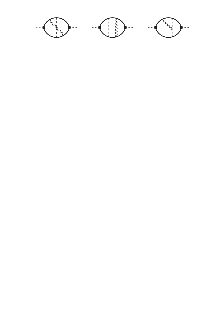
Figure 1: Three-loop diagrams generating an overall divergence proportional to $\alpha_{s}^{2}E/\epsilon$. Thick lines denote an unstable top-quark propagator, wavy (dashed) lines ultrasoft (potential) gluons; the square the non-relativistic current insertion. Symmetric versions of the last two diagrams are not displayed.

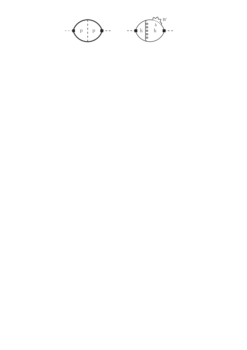
Figure 2: Cancellation of the overall divergence $\alpha_{s}E/\epsilon$ at NNLO against a partially “non-resonant” electroweak contribution involving a $Wb$ top-quark self energy insertion. Symmetric versions of the last diagram are not displayed.

The issue for top quarks is its large decay width $\Gamma_{t}\sim 1.4\,\mbox{GeV}$, which happens to be of order of the relevant non-relativistic energies $E$. The correct prescription for the calculation of the ultrasoft correction is to replace $E\to E+i\hskip 0.85355pt\Gamma_{t}$ in all equations [4]. Equivalently, we may consider $E$ to be complex with a finite imaginary part rather than the $+i\epsilon$-prescription for stable quarks. Now, the ultrasoft calculation yields an overall divergence (arising from quadratically divergent three-momentum integrals)

$$[\delta^{us}G(E)]_{\rm overall}\propto\frac{\alpha_{s}^{2}}{\epsilon}\cdot E$$ (3)

from the three-loop diagrams shown in Figure 1. If $E$ is complex, this results in a divergence $\alpha_{s}^{2}\Gamma_{t}/\epsilon$ in the heavy-quark production cross section (2) that is not cancelled by any counterterm associated with the heavy-quark currents. A similar overall divergence has already appeared in NNLO calculations of top-quark pair production such as [9], where it arises from two-loop diagrams with both loops in the potential region as shown in the first diagram in Figure 2. The origin and cancellation of such divergences is best understood in unstable-particle effective field theory [10], which provides a consistent treatment of finite-width effects beyond the $E\to E+i\hskip 0.85355pt\Gamma_{t}$ replacement (valid only up to NLO), and includes non-resonant contributions to physical cross sections, here $e^{+}e^{-}\to W^{+}W^{-}b\bar{b}$, which do not include the unstable top quark in the final state. In this framework, the overall ultraviolet divergence $\alpha_{s}\Gamma_{t}/\epsilon$ from the first diagram in Figure 2 is cancelled against an infrared divergence from the second diagram. Note that the second diagram is not present in non-relativistic QCD or for stable quarks, since all loops are in the hard region, and that the electroweak self-energy insertion is computed in conventional perturbation theory in the full standard model. The second diagram is ${\cal O}(\alpha_{s}\alpha_{w})$, so the parameter dependence matches, since $\Gamma_{t}\propto\alpha_{w}$, where $\alpha_{w}$ denotes the SU(2) gauge coupling. A similar cancellation between the overall divergences from Figure 1 with non-resonant contributions is expected at NNNLO.

The ultrasoft contribution to the NRQCD correlation function provides only part of the third-order result for the heavy-quark pair production cross section near threshold, and is regularization- and scheme-dependent. Our conventions for dimensional regularization and the counterterms have been specified in [1] and are chosen to conform with standard conventions for the calculation of $\overline{\rm MS}$-subtracted coefficient functions. With respect to the overall divergences discussed above, we note that we perform the calculation of the correlation function (1) with NRQCD for stable quarks in the complex energy plane at $E+i\hskip 0.85355pt\Gamma_{t}$. This corresponds to keeping only the leading width-correction in the effective Lagrangian for unstable quarks, $(i\Gamma_{t}/2)\,\psi^{\dagger}\psi$, in the framework [10]. The $1/\epsilon$ poles are then subtracted minimally ($\overline{\rm MS}$). The resulting scheme and scale dependence cancels with other NRQCD contributions to the correlation function, and matching coefficients, but there is a left-over dependence proportional to $\Gamma_{t}$ due to the overall divergences discussed above, which cancels with electroweak corrections that are not yet known.

We are now in the position to present our main result. (The technical details of the calculation will be explained together with those of [1] in a separate publication.) We express this in terms of the dimensionless complex energy variable $\hat{E}\equiv E/(m\alpha_{s}^{2})$, where $\mbox{Im}\,\hat{E}=\hat{\Gamma}_{t}=\Gamma_{t}/(m\alpha_{s}^{2})$, and

$$\lambda=\frac{C_{F}}{2\sqrt{-\hat{E}}},\qquad{\cal P}=\ln\left(\frac{C_{F}}{\lambda}\right)+\gamma_{E}+\psi(1-\lambda),$$ (4)

with $C_{F}=4/3$, and $\psi(z)\equiv d\Gamma(z)/dz$ the $\psi$-function ($\psi^{\,\prime}(z)$ denotes its first derivative). $\hat{G}_{C}=(2/3)(1-1/\lambda-2\,{\cal P})$, used below, is related to the Coulomb Green function at zero radial distance by $G_{C}=m^{2}\alpha_{s}/(4\pi)\,\hat{G}_{C}$. The imaginary part of the correlation function at complex energy involves divergent, logarithmic and finite contributions. We obtained the divergent and logarithmic terms in closed form and the remainder numerically. We thus obtain

$$\delta^{us}G(E) = \frac{2m^{2}\alpha_{s}^{4}}{9\pi^{2}}\Bigg{\{}\,\bigg{[}\frac{17\,i\hat{\Gamma}_{t}}{24}+\frac{527\,\hat{G}_{C}}{72}\bigg{]}\,\frac{1}{\epsilon^{2}}+\,\bigg{[}\frac{17\,i\hat{\Gamma}_{t}}{12}+\frac{221\,\hat{G}_{C}}{36}\bigg{]}\,\frac{1}{\epsilon}\,\ln\frac{\mu}{m}$$ (5)

$$+\,\bigg{[}\bigg{(}\frac{19}{12}\,\ln 2-\frac{91}{72}\bigg{)}\,i\hat{\Gamma}_{t}+\bigg{(}-\frac{119}{12}\,\ln 2+\frac{2059}{108}\bigg{)}\,\hat{G}_{C}\bigg{]}\,\frac{1}{\epsilon}$$

$$+\,\bigg{[}-\frac{34\,i\hat{\Gamma}_{t}}{3}-\frac{595\,\hat{G}_{C}}{9}\bigg{]}\,\ln^{2}\alpha_{s}+\bigg{[}-\frac{17\,i\hat{\Gamma}_{t}}{12}-\frac{833\,\hat{G}_{C}}{36}\bigg{]}\,\ln^{2}\frac{\mu}{m}$$

$$+\,\bigg{[}\frac{34\,i\hat{\Gamma}_{t}}{3}+\frac{748\,\hat{G}_{C}}{9}\bigg{]}\,\ln\alpha_{s}\ln\frac{\mu}{m}$$

$$+\,\bigg{[}\frac{2380\,{\cal P}^{2}}{27}+\left(\frac{272\ln{2}}{9}-\frac{23483}{162}+\frac{2380}{27\lambda}+\frac{272}{27\lambda^{2}}\right){\cal P}+\left(\frac{27\lambda}{2}-\frac{16}{3\lambda}\right)\psi^{\,\prime}(1-\lambda)$$

$$+\frac{64}{27\lambda^{3}}+\frac{4\,(-1331+306\ln{2})}{81\lambda}+\frac{4\,(-199+114\ln{2})}{81\lambda^{2}}\bigg{]}\,\ln\alpha_{s}$$

$$+\,\bigg{[}-\frac{1496\,{\cal P}^{2}}{27}+\left(-\frac{34\ln{2}}{3}+\frac{5065}{72}-\frac{1496}{27\lambda}-\frac{136}{27\lambda^{2}}\right){\cal P}+\left(\frac{8}{3\lambda}-\frac{81\lambda}{8}\right)\psi^{\,\prime}(1-\lambda)$$

$$-\frac{32}{27\lambda^{3}}+\frac{163-114\ln{2}}{27\lambda^{2}}+\frac{271-51\ln{2}}{9\lambda}\bigg{]}\,\ln\frac{\mu}{m}+\,\delta^{us}(\hat{E})\Bigg{\}}.$$

The double logarithmic and $1/\epsilon$ pole terms are identical to those that appear in the result for the wave function at the origin (Eqn. (13) of [1]) under the replacements $\Gamma_{t}\to 0$, $\hat{G}_{C}\to K\equiv(8/9)\,(\alpha_{s}^{3}/\pi)\,|\psi_{n}^{C}(0)|^{2}/\left(2m^{2}\alpha_{s}^{4}/(9\pi^{2})\right)$. By expanding $\delta^{us}G(E)$ around the bound-state poles $\lambda=n$, we also reproduce the single logarithmic terms in [1]. Only the imaginary part of $\delta^{us}G(E)$ is needed for the cross section (2), therefore in writing (5) we already dropped some purely real terms. The imaginary part of the non-logarithmic correction $\delta^{us}(\hat{E})$ is tabulated in Table 1 for a set of values of the real part (rows) and imaginary part (columns) of $\hat{E}$ in a range relevant to top-quark pair production. The table can be used to generate an interpolating function with an accuracy better than 0.1 in the entire range of the table.

$\mbox{Re}\,\hat{E}\;\backslash\;\hat{\Gamma}_{t}$ 0.343 0.443 0.543 0.643 0.743 -4.10 2.282 2.790 3.182 3.432 3.521 -3.90 5.542 6.966 8.247 9.357 10.27 -3.70 9.255 11.72 14.00 16.07 17.91 -3.50 13.53 17.18 20.60 23.76 26.62 -3.30 18.51 23.53 28.26 32.66 36.68 -3.10 24.40 31.01 37.26 43.08 48.42 -2.90 31.46 39.97 47.99 55.45 62.28 -2.70 40.09 50.87 61.00 70.37 78.90 -2.50 50.87 64.42 77.06 88.66 99.13 -2.30 64.68 81.65 97.33 111.5 124.2 -2.10 82.90 104.2 123.6 140.8 155.8 -1.90 107.8 134.7 158.5 179.1 196.5 -1.70 143.6 177.5 206.5 230.5 249.8 -1.50 197.8 240.5 274.9 301.4 320.8 -1.30 285.8 338.2 375.8 400.8 415.8 -1.10 441.4 497.2 527.3 539.5 540.1 -1.00 565.1 612.6 628.2 625.5 612.9 -0.96 627.4 667.2 673.7 662.6 643.4 -0.92 698.6 727.1 721.8 701.1 674.4 -0.88 779.8 792.1 772.3 740.4 705.6 -0.84 871.7 862.0 824.6 780.1 736.6 -0.80 974.9 936.0 877.8 819.6 767.0 -0.76 1089. 1013. 930.7 858.1 796.4 -0.72 1211. 1089. 982.1 894.8 824.3 -0.68 1336. 1164. 1030. 928.8 850.1 -0.64 1458. 1231. 1073. 959.3 873.5 -0.60 1565. 1288. 1109. 985.3 893.9 -0.56 1643. 1329. 1137. 1006. 911.2

$\mbox{Re}\,\hat{E}\;\backslash\;\hat{\Gamma}_{t}$ 0.343 0.443 0.543 0.643 0.743 -0.52 1681. 1352. 1155. 1022. 925.0 -0.48 1673. 1356. 1163. 1032. 935.4 -0.44 1620. 1341. 1162. 1037. 942.4 -0.40 1534. 1311. 1153. 1036. 946.2 -0.36 1433. 1271. 1138. 1032. 947.1 -0.32 1332. 1226. 1118. 1024. 945.7 -0.28 1243. 1180. 1095. 1014. 942.1 -0.24 1169. 1137. 1072. 1002. 937.1 -0.20 1112. 1099. 1049. 989.3 931.0 -0.16 1070. 1065. 1027. 976.4 924.0 -0.12 1038. 1037. 1007. 963.7 916.7 -0.08 1015. 1014. 989.0 951.4 909.2 -0.04 996.8 994.4 972.9 939.9 901.7 0.00 982.4 978.0 958.7 929.2 894.4 0.10 955.4 946.6 929.7 905.8 877.4 0.30 918.9 906.4 890.6 871.7 850.1 0.50 893.4 880.3 865.3 848.7 830.4 0.70 874.4 861.5 847.4 832.2 816.0 0.90 859.8 847.3 834.0 819.9 805.2 1.10 848.3 836.4 823.8 810.7 797.0 1.30 839.2 827.8 816.0 803.6 790.9 1.50 832.2 821.3 810.0 798.3 786.3 1.70 826.7 816.3 805.5 794.4 783.1 1.90 822.5 812.5 802.3 791.7 781.0 2.10 819.5 810.0 800.1 790.1 779.8 2.30 817.6 808.3 798.9 789.3 779.4 2.50 816.5 807.6 798.5 789.3 779.8 2.70 816.2 807.6 798.9 790.0 780.9

Table 1: Value of the non-logarithmic ultrasoft correction $\mbox{Im}\,\delta^{us}(\hat{E})$ for various scaled energies $\hat{E}=E/(m\alpha_{s}^{2})$. Columns refer to different $\mbox{Re}\,\hat{E}$ from $-4.1$ to $2.7$, rows to five values of $\mbox{Im}\,\hat{E}=\hat{\Gamma}_{t}=\Gamma_{t}/(m\alpha_{s}^{2})$ for given real part.

The new ultrasoft correction has a very large effect on the $t\bar{t}$ cross section near threshold as illustrated in Figure 3. Here we adopt the top quark pole mass $m_{t}=175\,$GeV, and fix $\alpha_{s}=0.14$, which corresponds to the Bohr radius scale $\mu_{B}=32.5\,$GeV. The solid line in the upper panel of Figure 3 shows the non-logarithmic contribution from $\mbox{Im}\,\delta^{us}(\hat{E})$ to $[R]_{us}$ alone, which is seen to be around $+25\%$ in the peak region, in nice agreement with the estimate from the wave-function calculation [1]. Including the logarithmic term requires a choice of the scale $\mu$. Since $\mu$ is not related to the scale of $\alpha_{s}$, but designates a factorization scale that separates the ultrasoft from hard and potential contributions, we choose the two values $\mu_{B}$ and $m_{t}$ to represent a reasonable range. Since the factorization scale dependence is sizable this results in a large range of $[R]_{us}$ reflected in the two dashed curves in Figure 3 (upper panel). We add these two results to the leading order $t\bar{t}$ cross section in the lower panel. Our results show that despite the large quark mass, third-order perturbative corrections from the ultrasoft scale can have a significantly larger impact on top-quark pair production than anticipated. However, it should be kept in mind that the ultrasoft correction is not physical by itself as is clear from its factorization scale dependence. (The non-logarithmic term is still factorization-scheme dependent.) In [11] we combined the ultrasoft correction reported here with the third-order potential correction [12] and all other calculated third-order terms and observed a significant cancellation between the ultrasoft and potential terms. A final assessment of theoretical uncertainties should therefore be attempted only once all third-order corrections to the $t\bar{t}$ cross section have been assembled.

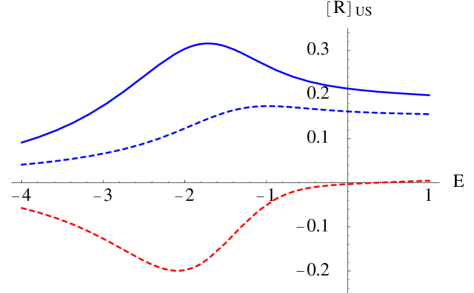
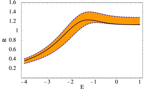
Figure 3: Top panel: Ultrasoft correction $[R]_{us}$ to $t\bar{t}$ production as function of $E=\sqrt{s}-2m_{t}$. Solid: non-logarithmic contribution only. Dashed: total contribution with $\mu=\mu_{B}=32.6\,$GeV (upper dashed) and $\mu=m_{t}=175\,$GeV (lower dashed). Parameters: $m_{t}=175\,$GeV, $\Gamma_{t}=1.4\,$GeV, $\alpha_{s}=0.14$. Bottom panel: Ultrasoft correction added to the leading order (LO) cross section, i.e. $[R]_{\rm LO}+[R]_{us}$. The band is obtained by varying the scale $\mu$ between $\mu_{B}$ (upper line) to $m_{t}$ (lower line). The solid black line refers to the LO cross section.

The heavy-quark correlation function near threshold is also a crucial input to the determination of $m_{b}$ from large-moment bottomonium sum rules [13]. The $n$th moment of the $b\bar{b}$ production cross section is defined by

$${\cal M}_{n}/(10\,\mbox{GeV})^{2n} \equiv \frac{12\pi^{2}}{n!}\,\frac{d^{n}}{d(q^{2})^{n}}\,\Pi(q^{2})_{\big{|}q^{2}=0}=\int\limits_{0}^{\infty}\!\frac{ds}{s^{n+1}}\,R_{b\bar{b}}(s).$$ (7)

Taking large $n$, typically $n\geq 4$, enhances the sensitivity to $m_{b}$ and the threshold region, but requires a non-relativistic treatment to sum corrections of order $\alpha_{s}\sqrt{n}$ to all orders in perturbation theory. On the other hand $n$ cannot be too large, since $m_{b}/n$, the typical non-relativistic energy of a $b\bar{b}$ pair contributing to the $n$th moment must be larger than $\Lambda_{\rm QCD}$ to justify a perturbative computation [14]. To calculate the derivatives of the QCD vector current correlation function $\Pi(q^{2})$, we evaluate the moment integral in (7) with $R_{b\bar{b}}(s)$ expressed as a sum over Coulomb resonances and a continuum for $E=\sqrt{s}-2m_{b}>0$, which should be dual to the corresponding integrated physical $b\bar{b}$ cross section.

The ultrasoft correction $[R]_{us}$ to the continuum cross section is obtained from (2) and

$$\mbox{Im}\;\delta^{us}G(E)=\lim_{\Gamma\to 0+}\,\mbox{Im}\;\delta^{us}G(E+i\hskip 0.85355pt\Gamma)\qquad(E>0).$$ (8)

While we have an analytic representation of the logarithmic contributions, see (5), our numerical implementation of the non-logarithmic term $\delta^{us}(\hat{E})$ does not allow us to make the imaginary part of $\hat{E}$ arbitrarily small. We therefore calculate $\delta^{us}G(E+i\hskip 0.85355pt\Gamma)$ for several values of $\Gamma$ (for given $E$) and obtain the continuum value by extrapolating to $\Gamma=0$ through a polynomial fit. By variations of this procedure we estimate that the relative error in the calculation of the ultrasoft contribution to the continuum cross section (real $E>0$) is less than $1\%$. Numbers for the non-logarithmic term are provided in Table 2.

$\hat{E}$ $\mbox{Im}\,[\delta^{us}]$ 0 979.0 0.05 973.5 0.10 968.7 0.20 958.6 0.30 948.3 0.40 938.3 0.50 928.7

$\hat{E}$ $\mbox{Im}\,[\delta^{us}]$ 0.70 911.5 0.90 896.9 1.10 884.7 1.30 874.7 1.50 866.5 1.70 859.9 1.90 854.6

$\hat{E}$ $\mbox{Im}\,[\delta^{us}]$ 2.10 850.5 2.50 845.0 3.10 843.6 3.70 848.0 4.30 857.8 4.90 871.3 5.50 888.0

$\hat{E}$ $\mbox{Im}\,[\delta^{us}]$ 6.10 908.2 6.80 935.7 8.00 990.0 9.00 1042.5 10.0 1101.1 12.0 1234.8 14.0 1388.3

Table 2: Values of the non-logarithmic ultrasoft correction $\mbox{Im}\,[\delta^{us}(\hat{E}+i\epsilon)]$ in the continuum (real positive $\hat{E}$).

$n$	6	10	14
${\cal M}_{n}^{\rm LO}$	0.134	0.122	0.139
${\cal M}_{n}^{\rm LO+US}$	0.178	0.190	0.250

Table 3: Moments of the $b\bar{b}$ spectral function for $m_{b}=4.95\,\mbox{GeV}$. (The moment integral is cut off at $\hat{E}=20$.) The renormalization/factorization scale is taken to be $\mu_{n}=2m_{b}/\sqrt{n}$ corresponding to $\alpha_{s}(\mu_{n})=0.228,0.250,0.267$ for $n=6,10,14$. The last row shows the sum of the leading-order moments and the ultrasoft contribution. The leading order alone is given in the first row for comparison [14].

The sum of the leading-order and ultrasoft contribution to the moments is given in Table 3 together with the leading-order one alone for $b$-quark pole mass $m_{b}=4.95\,\mbox{GeV}$ and renormalization/factorization scale $\mu_{n}=2m_{b}/\sqrt{n}$. Given the large size of the ultrasoft term in the $t\bar{t}$ cross section it may not be surprising that here we find that the ultrasoft correction is 30% to 80% of the leading-order term, putting the perturbative approach into doubt for the larger moments. (The correction from the non-logarithmic term alone is even larger, cf. Figure 3, upper panel.) However, as mentioned above, the result for the ultrasoft correction alone should be regarded with caution, and there is reason for assuming that the large ultrasoft correction is partially a consequence of $\overline{\rm MS}$ factorization, such that the true third-order correction is smaller when all other corrections are added.

To summarize, we evaluated the correction to the vector-current heavy-quark correlation function from ultrasoft gluon exchange, which appears first at NNNLO in the non-relativistic expansion, and is required for accurate top and bottom quark mass determinations from the threshold pair production cross section. The correction turns out to be large even for top quarks, but a definite conclusion on the attainable theoretical precision can only be drawn once the full NNNLO result, including potential and hard corrections, is available. A discussion of the sum of all known NNNLO terms for top quark production can be found in [11].

References

- [1] M. Beneke, Y. Kiyo and A. A. Penin, Phys. Lett. B 653 (2007) 53, arXiv:0706.2733 [hep-ph].
-
[2]
B. A. Kniehl and A. A. Penin,
Nucl. Phys. B 563 (1999) 200
[hep-ph/9907489];
B. A. Kniehl, A. A. Penin, V. A. Smirnov and M. Steinhauser, Nucl. Phys. B 635 (2002) 357 [hep-ph/0203166]. - [3] V.A. Novikov et al., Phys. Rev. Lett. 38 (1977) 626 [Erratum: ibid. 38 (1977) 791]; Phys. Rep. 41 (1978) 1.
- [4] V.S. Fadin and V.A. Khoze, Pis’ma Zh. Eksp. Teor. Fiz. 46, 417 (1987) [JETP Lett. 46, 525 (1987)]; Yad. Fiz. 48, 487 (1988) [Sov. J. Nucl. Phys. 48(2), 309 (1988)].
- [5] M. Beneke, “Perturbative heavy quark-antiquark systems,” in: Proceedings of the 8th International Symposium on Heavy Flavor Physics (Heavy Flavors 8), Southampton, England, 25-29 Jul 1999 [hep-ph/9911490].
- [6] A. H. Hoang et al., Eur. Phys. J. direct C 2 (2000) 1 [hep-ph/0001286].
- [7] M. Beneke and V. A. Smirnov, Nucl. Phys. B 522 (1998) 321 [hep-ph/9711391].
- [8] A. H. Hoang and C. J. Reisser, Phys. Rev. D 71 (2005) 074022 [hep-ph/0412258].
- [9] M. Beneke, A. Signer and V. A. Smirnov, Phys. Lett. B 454 (1999) 137 [hep-ph/9903260].
- [10] M. Beneke, A. P. Chapovsky, A. Signer and G. Zanderighi, Phys. Rev. Lett. 93 (2004) 011602 [hep-ph/0312331]; Nucl. Phys. B 686 (2004) 205 [hep-ph/0401002].
-
[11]
M. Beneke, Y. Kiyo and K. Schuller,
arXiv:0801.3464 [hep-ph], to be published in: Proceedings of 8th
International Symposium on Radiative Corrections (RADCOR 2007):
Application of Quantum Field Theory to Phenomenology, Florence,
Italy, 1-6 Oct 2007;
M. Beneke, Y. Kiyo, A. Penin and K. Schuller, arXiv:0710.4236 [hep-ph], in: Proceedings of 2007 International Linear Collider Workshop (LCWS07 and ILC07), Hamburg, Germany, 30 May - 3 Jun 2007. - [12] M. Beneke, Y. Kiyo and K. Schuller, in preparation.
-
[13]
M.B. Voloshin and Yu.M. Zaitsev, Usp. Fiz. Nauk. 152 (1987) 361
[Sov. Phys. Usp. 30(7) (1987) 553];
M.B. Voloshin, Int. J. Mod. Phys. A10 (1995) 2865. - [14] M. Beneke and A. Signer, Phys. Lett. B 471 (1999) 233 [hep-ph/9906475].