The Kinematics of Thick Disks in Nine External Galaxies

Abstract

We present kinematic measurements of thin and thick disk components in a sample of nine edge-on galaxies. We extract stellar and ionized gas rotation curves at and above the galaxies’ midplanes using the Ca ii triplet absorption features and H$\alpha$ emission lines measured with the GMOS spectrographs on Gemini North and South. For the higher mass galaxies in the sample, we fail to detect differences between the thin and thick disk kinematics. In the lower mass galaxies, there is a wide range of thick disk behavior including thick disks with substantial lag and one counter-rotating thick disk. We compare our rotation curves with expectations from thick disk formation models and conclude that the wide variety of thick disk kinematics favors a formation scenario where thick disk stars are accreted or formed during merger events as opposed to models that form thick disks through gradual thin disk heating.

1. Introduction

The detailed distribution of stars in galaxies gives vital information regarding their formation and subsequent evolution. Of particular interest are the oldest stellar populations, which in the Milky Way are the thick disk and halo. These old components provide the best record of early galaxy assembly. Originally detected in edge-on S0 galaxies (Burstein, 1979; Tsikoudi, 1979), thick stellar disks have now been found in a wide variety of galaxies–S0’s (de Grijs & van der Kruit, 1996; de Grijs & Peletier, 1997; Pohlen et al., 2004), Sb’s (van der Kruit, 1984; Shaw & Gilmore, 1989; van Dokkum et al., 1994; Morrison et al., 1997; Wu et al., 2002), and later type galaxies (Dalcanton & Bernstein, 2002; Abe et al., 1999; Neeser et al., 2002; Yoachim & Dalcanton, 2006). Observations with HST have allowed thick disks in other galaxies to be studied as resolved population (Seth et al., 2005, 2007; Tikhonov et al., 2005; Tikhonov & Galazutdinova, 2005; Mould, 2005), while observations at high redshift show potential thick disks in the process of forming (Elmegreen & Elmegreen, 2006).

The most detailed studies of thick disks come from observations within the Milky Way. Since its discovery (Gilmore & Reid, 1983), the MW thick disk has been found to be structurally, chemically, and kinematically distinct from the thin disk. Structurally, star counts with large surveys such as SDSS and 2MASS reveal the galaxy is best fit with two disk components (e.g., Ojha, 2001; Jurić et al., 2008). Chemically, thick disk stars are more metal-poor and older than stars in the thin disk (e.g., Reid & Majewski, 1993; Chiba & Beers, 2000). They are also significantly enhanced in $\alpha$-elements, compared to thin disk stars of comparable iron abundance (Prochaska et al., 2000; Tautvaišienė et al., 2001; Bensby et al., 2003; Feltzing et al., 2003; Mishenina et al., 2004; Brewer & Carney, 2004; Bensby et al., 2005; Brewer & Carney, 2006; Ramírez et al., 2007). Kinematically, thick disk stars have both a larger velocity dispersion and slower net rotation than stars in the thin disk (Nissen, 1995; Chiba & Beers, 2000; Gilmore et al., 2002; Soubiran et al., 2003; Parker et al., 2004; Girard et al., 2006). All of these facts lead to the conclusion that the thick disk is a relic of the young Galaxy. As such, it provides an excellent probe of models of disk galaxy formation (see reviews by Nissen et al. (2003); Freeman & Bland-Hawthorn (2002)).

Given these systematic differences between their properties, thick and thin disks are likely to have distinct formation mechanisms. The structure, dynamics, and chemical abundance of the thin disk strongly suggest that the majority of its stars formed gradually from a thin rotating disk of high angular momentum gas (Fall & Efstathiou, 1980; Chiappini et al., 1997; Cescutti et al., 2007). In contrast, the formation of the thick disk is still poorly constrained and is likely to be more complex.

Thick disk formation models can be grouped into three broad categories. In the first, a previously thin disk is kinematic heated. In this scenario, stars form in a thin disk and increase their velocity dispersion with time. This vertical heating can be rapid, due to interactions and mergers (Quinn et al., 1993; Walker et al., 1996; Velazquez & White, 1999; Chen et al., 2001; Robin et al., 1996) or gradual, due to scattering off giant molecular clouds, spiral arms, and/or dark matter substructure (Villumsen, 1985; Carlberg, 1987; Hänninen & Flynn, 2002; Benson et al., 2004; Hayashi & Chiba, 2006; Kazantzidis et al., 2007). In the second formation scenario, stars “form thick” with star formation occurring above the midplane of the galaxy (Brook et al., 2004) or form with large initial velocity dispersions in large stellar clusters (Kroupa, 2002). In the final class of models, thick disk stars are directly accreted from satellite galaxies. Numerical simulations have shown that stars in disrupted satellite galaxies can be deposited onto thick disk like orbits (Abadi et al., 2003; Martin et al., 2004; Bekki & Chiba, 2001; Gilmore et al., 2002; Navarro et al., 2004; Statler, 1988), producing extended stellar debris such as seen around M31 (Ibata et al., 2005; Kalirai et al., 2006; Ferguson et al., 2002). While these models were originally developed to explain the origin of the MW thick disk, they should work equally well for thick disks in other galaxies.

Measuring the kinematics of thick disk stars is one of the best discriminators between the formation models. If the thick disk forms from a heated thin disk, we expect the kinematics of the two components to be closely related. On the other hand, if the thick disk stars form outside the galaxy and are later accreted, we could find systems where the thick disk kinematics are completely decoupled from the thin disk.

In this paper, we present observations of stellar and gas kinematics in nine edge-on systems as part of our continuing analysis of thick disks in a large sample of edge-on galaxies (Dalcanton & Bernstein, 2000). Compared to Yoachim & Dalcanton (2005), which presented the first two galaxies in this study, we have improved the analysis techniques and significantly expanded our sample size.

2. Observations

2.1. Target Selection

We have carried out long-slit spectroscopic observations using the Gemini North and South telescopes of nine galaxies drawn from the Dalcanton & Bernstein (2000) sample of edge-on late-type galaxies. The original sample of 49 galaxies was selected from the Flat Galaxy Catalog (Karachentsev et al., 1993) and imaged in $B$, $R$, and $K_{s}$ (Dalcanton & Bernstein, 2000). This sample was selected to contain undisturbed pure disk systems spanning a large range of mass. Dalcanton & Bernstein (2002) used this imaging to demonstrate the ubiquity of thick disks around late-type galaxies, while Yoachim & Dalcanton (2006) used two-dimensional photometric decompositions to measure the structural parameters for the thick and thin disks. All the galaxies in the sample presented here have prominent thin star forming disks.

Our spectroscopic program targeted galaxies spanning a wide range of masses ($50<V_{c}<150$ km s^-1). The sample targets were limited to those that had thick disks that we believed we could isolate adequately–i.e., those that had significantly larger scale heights from the thin disk and that were bright enough that we could acquire spectra in reasonable observing times. This constraint caused several of the higher mass galaxies to be rejected from the kinematic sample, as the regions where the thick disk could be expected to dominate were simply too faint. This bias is consistent with the conclusion of Yoachim & Dalcanton (2006) that the thick disk is more prevalent in lower mass galaxies. Our selection criterion limited the sample to $\sim$20 galaxies of the original 49. We also selected galaxies to be at redshifts such that the Ca features did not land on night sky emission lines. In our initial observations, we submitted more galaxies than we could observe and let the Gemini observing specialists select which galaxies would best fit with the queue scheduling. For the final observing runs we explicitly selected galaxies to ensure that a reasonable mass range was observed in the final sample. The properties of the final sample are listed in Table 1.

2.2. Observing Strategy

Based on the thin and thick disk decompositions in Yoachim & Dalcanton (2006), we targeted regions of the galaxies where the flux is dominated by either the thin or thick disk stars. The two highest mass galaxies in our sample have notable dustlanes (Dalcanton et al., 2004), and for these we offset the spectra slit to observe regions of the galaxy which should be optically transparent. We discuss possible residual dust effects in detail in § 7. When selecting slit placement for the offplane, the direction of offset was based primarily on avoiding foreground objects and the ability to use a single guide star for all dither positions.

For our instrumental setup, we used GMOS on Gemini North in longslit mode with a 0.5^′′ slit and the R400_G5305 grating set to a central wavelength of $\sim 8440$ Å along with the OG515_G0306 filter. Similarly for observations from Gemini South, we used a 0.5^′′ slit the R400+_G5325 grating and OG515_G0330 filter. For both GMOS setups, we binned the CCDs by 2 in the spatial direction during readout giving a pixel scale of 0.145^′′/pix in the spatial direction and 0.69 Å/pixel in the spectral direction. The resulting spectra cover the wavelength range of $\sim 6330-10570$ Å, although there is heavy residual fringing redward of 9300 Å. Exposure times for individual frames were 900, 1200, or 1800 seconds. The midplanes were observed 3-5 times while offplane positions were observed 18-51 times depending on the galaxy. Exposures were spatially dithered $\sim$30^′′ along the slit. These configurations allow us to simultaneously observe the H$\alpha$ emission and Ca ii triplet absorption features out to large radii.

All of the observations were executed in queue mode over five semesters. The observation details for each galaxy are listed in Table 2, with details of the slit positions listed in Table 3.

Table 1Properties of Targeted Galaxies

Galaxy	Dist1	Vc	$h_{R}$	$z_{0,thin}$	$z_{0,thick}$	$L_{thick}/L_{thin}$
FGC	Mpc	km s-1	′′	′′	′′
227	89.4	106.0	10.2	1.8	3.9	0.47
780	34.4	75.0	15.1	3.1	8.4	0.93
1415	38.3	86.5	18.3	2.8	6.6	0.95
1440	70.9	150.5	15.9	2.3	5.0	0.38
1642	36.6	55.0	12.5	3.1	10.0	0.19
1948	36.9	54.5	12.3	1.6	3.6	3.56
2558	73.8	89.0	9.2	2.6	3.6	0.47
E1371	82.6	131.0	7.7	1.6	3.4	0.27
E1498	135.5	133.0	7.6	1.2	3.8	0.19

¹Karachentsev et al. (2000)

Table 2Observing Details

Galaxy	Gemini ID	Observation Dates	Midplane Exposure	Offplane Exposure
FGC			# x time (s)	# x time (s)
1415	GN-2003A-Q-6	3-28-2003 to 06-06-2003	3x900	41x1200
227	GN-2003B-Q-51	9-21-2003 to 11-22-2003	3x1200	27x1200
1642	GN-2004A-Q-54	02-16-2004 to 06-24-2004	3x1200	51x1200
780	GN-2004A-Q-54	02-20-2004 to 04-27-2004	5x1200	31x1200
2558	GN-2004B-Q-29	07-15-2004 to 11-20-2004	3x1200	36x1200
E1498	GS-2004B-Q-44	03-11-2005 to 06-10-2005	3x1200	50x1200
1948	GN-2005A-Q-21	08-12-2004 to 08-24-2004	5x1800	18x1800
E1371	GS-2005A-Q-17	04-05-2005 to 04-14-2005	3x1200	21x1800
1440	GS-2005A-Q-17	02-11-2005 to 04-05-2005	3x1200	30x1800

Table 3Slit Placement

Galaxy	Midplane Offset1		Offplane Offset
FGC	arcsec	kpc	arcsec	kpc	$z/z_{0,thin}$	$z/z_{0,thick}$
227	0.0	0.0	3.0	1.3	1.7	0.8
780	0.0	0.0	6.5	1.1	2.1	0.8
1415	0.0	0.0	5.4	1.0	1.9	0.8
1440	0.5	0.2	4.5	1.5	2.0	0.9
1642	0.0	0.0	4.2	0.7	1.4	0.4
1948	0.0	0.0	3.1	0.6	1.9	0.9
2558	0.0	0.0	3.9	1.4	1.5	1.1
E1371	0.5	0.2	2.8	1.1	1.8	0.8
E1498	0.0	0.0	2.0	1.3	1.7	0.5

¹Midplane offset to avoid obvious dust lanes.

2.3. Data Reduction

A combination of Gemini IRAF packages, standard IRAF packages, and custom IDL code were used to reduce our data. These procedures have been improved since initial results for FGC 227 and FGC 1415 were published in Yoachim & Dalcanton (2005) and have been applied to the entire data set. We bias corrected the images using a fit determined from the overscan region followed by subtracting residual structure measured from a bias frame. Because both GMOS North and South are extremely stable, we were able to create average bias images by combining $\sim$60 bias frames per observing semester. We interpolated the three GMOS chips into a single image using the Gemini IRAF tasks, after which the standard IRAF reduction tools were used. For Gemini-South observations, we also needed to subtract a dark current correction of $\sim$6-12 counts from the science frames. Gemini-North images showed no detectable dark current. Images were flat-fielded using GCAL lamp flats that were taken every hour interspersed with the science observations, minimizing the amount of fringing present in the final frames. We applied a slit illumination correction using twilight sky observations.

For wavelength calibration, we used the night-sky atlases of Osterbrock et al. (1996) and Osterbrock et al. (1997) to create a sky line list containing only lines (or stable unresolved doublets) that could be centroided with our instrumental set-up. For each science exposure, we identified 100-110 sky lines to use for rectification. We then used these lines for a 5th order Legendre polynomial fit for wavelength calibration, and rebinned our spectra to a common dispersion. Typical dispersions were 0.69 Å pixel^-1 with calibration arc lamps showing a FWHM of 3.8 Å. The wavelength solutions were stable over each observing night.

Sky subtraction proved difficult because of the large number of strong sky emission lines. If we use standard sky subtraction techniques, we find that there are large systematic residuals left on our frames due to variation in the width of the slit along its length. The RMS deviation in the centroid position of a single sky line is $\sim$0.07 Å while the RMS of its Gaussian FWHM is 0.11 Å. This is a surprisingly high variation for the width of the slit. We have tried the sky-subtraction techniques described in Kelson et al. (2000) and find that the systematic residuals remain, although the Kelson et al. (2000) sky-subtraction technique does eliminate problems associated with wavelength rectification and interpolation. Having eliminated our data-reduction procedure as the cause, we conclude the high dispersion in sky line FWHM is indicative of a systematically varying slit width. In many cases, such residuals can be removed using the nod-and-shuffle technique (Glazebrook & Bland-Hawthorn, 2001). Unfortunately, our galaxies are too large ($\sim$1 arc minute, or 1/3 of the total slit width) to make effective use of traditional nod-and-shuffle.

To remove the systematic residuals present in the bright sky lines, we employ a nod-and-shuffle like template subtraction. Because we placed different galaxies on different spatial sections of the chips, all of the slit was illuminated by sky for at least some observations. We therefore could construct high S/N sky frames by masking objects in our 2-d spectra and combining the wavelength rectified frames. By doing this, we create a deep sky frame for each observing quarter. We then remove the sky background by selecting a sky-dominated region in a science frame and scaling the sky image column-by-column to match the science frame sky region, then subtract the rescaled sky frame from the science image. In most cases, we were forced to apply sky frames generated from different observing semesters to the science frames. Luckily, our instrument setup quarter-to-quarter was identical, and the GMOS instruments are stable enough that this technique works well at removing systematics caused by the variable slit width. This sky subtraction technique appears to give results comparable to nod-and-shuffle technique for individual frames. Our sky subtraction procedure incurs a small signal-to-noise penalty, but is effective at removing the systematic residuals from moderate sky lines (Figure 1).

This excessive agonizing over sky subtraction is demanded by the very low surface brightness levels of our targets. For an individual midplane image, the brightest part of the galaxy is $\sim 20\%$ brighter than the sky level, and for individual offplane images the signal is only $\sim 11\%$ the sky background. Examples of the spectra extracted over the central 14^′′ spatial extent of the galaxy before and after sky subtraction are shown in Figure 2.

When we combine several hours of observations we are more sensitive to low surface brightness features, and find some wavelengths are still dominated by systematic noise. Even with our sky template correction, some sky lines are so bright that some systematic residuals remain. When we use conventional sky-subtraction techniques, residual errors have maximum deviations of $\pm$55% while the template subtraction gives deviations of $\pm$38%. While deviations of 38% swamp out the signal from any stellar absorption lines near bright sky lines, the residual deviations for smaller sky lines are decreased to a level where the stellar absorption lines can be accurately measured. In Figure 1, we compare the two sky subtraction routines. The extracted spectra look similar, with both being dominated by the sky line residuals redward of 8750 Å. The template subtraction is able to eliminate the residuals left from the sky line at 8555 Å, just to the right of the weakest Ca ii triplet line, and reduces the large residuals at the reddest wavelengths plotted.

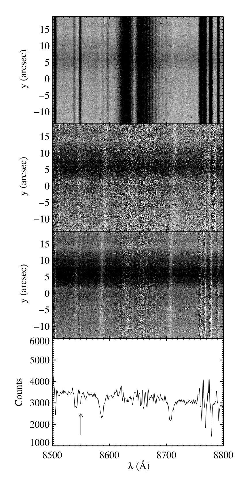
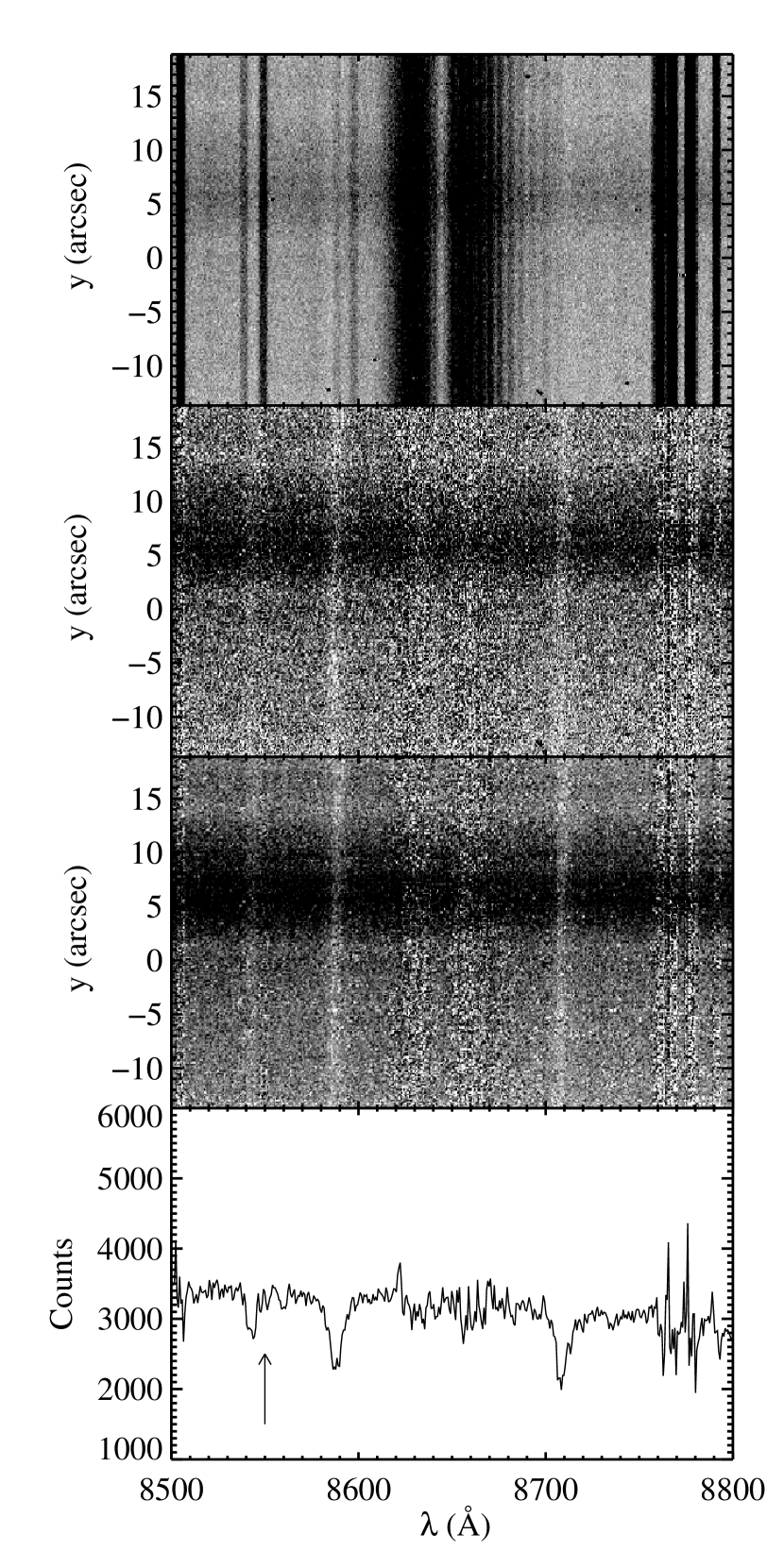
Figure 1.— Results from different sky subtraction techniques for the midplane of FGC 1415. On the left, we show the results from standard sky subtraction techniques and the right panels show our sky template subtraction. Top panels show the raw galaxy spectrum before the sky has been subtracted. Middle panels show a single subtracted frame and the final combined image. The bottom panel shows the combined spectrum summed along the spatial dimension. An arrow points out a sky line residual present in the standard subtraction that is eliminated in template subtraction. The brightest sky lines leave large residuals in both cases, but the magnitude of residuals is decreased significantly with the nod-and-shuffle-like technique (see the lines near $\sim 8770$ Å, for example).

Figure 2.— Examples of spectra before and after sky subtraction. The top panel shows the results of a single midplane exposure before and after sky template subtraction (top and middle curves respectively). The middle panel shows a single offplane exposure before and after extraction. Dotted lines show the RMS noise level in the spectra. The bottom panel shows the final midplane and offplane spectra after all the frames have been averaged together. The largest systematic residuals from the sky lines have been masked. The three vertical marks show the location of the Ca triplet absorption lines. All of the spectra were extracted over the central 14^′′ of the galaxy.

After the sky had been removed, the images were Doppler-corrected for motion relative to the Local Standard of Rest and combined. Before cross-correlation was performed, the spectra were rebinned into logarithmic wavelength bins.

3. Rotation Curves

3.1. H$\alpha$ Rotation Curves

Both our midplane and offplane observations show strong H$\alpha$ emission. For each galaxy, we extracted a series of 1-D spectra by summing 28 pixels ($\sim 4$^′′) along the spatial dimension. The ionized gas rotation curve was fit with a Gaussian peak to the H$\alpha$ line. In principle, an envelope-tracing method would produce a more robust measure of the rotation curve. However, we find that the width of the H$\alpha$ lines (FWHM$\sim$3.8 Å) are identical to the instrumental dispersion as measured from the arc lamps (FWHM$\sim$3.8 Å), and we would thus not gain much accuracy from a more detailed rotation curve extraction.

The [Nii] and [Sii] lines are present as well, but the H$\alpha$ line is so strong that we found no additional advantage in fitting all the emission lines simultaneously. We find typical uncertainties in the central wavelength of the H$\alpha$ Gaussian peak of 1-2 km s^-1 for midplane observations and 4-7 km s^-1 for offplane observations.

To double check the accuracy of our extracted rotation curve, we fit rotation curves to night sky lines before the background is subtracted off. Perfect calibration would result in sky line rotation curves with zero rotation. The central wavelengths of the sky lines vary with an RMS error of 2.4-3.5 km s^-1, with the higher value resulting from larger spatial extraction windows. Most of this scatter can be attributed to uncertainties in the wavelength rectification solution. With fewer sky lines around H$\alpha$ compared to the redder regions of our spectra, the rectification is not as well constrained. Overall, these tests suggest that we are able to extract the ionized gas rotation curve with an error of a few km s^-1.

The resulting H$\alpha$ rotation curves are plotted as solid lines in Figure 4. Our data show a tight agreement between the midplane and offplane H$\alpha$ curves, which is a good sign that dust is not obscuring the midplane rotation curves. If we were observing along major dustlanes, we could expect to see the offplane observations rotating faster than the midplane, especially at small galactic radii (see § 7).

We leave a detailed analysis of the gas kinematics for a later paper. At this time, we simply note that the midplane and offplane H$\alpha$ rotation curves are surprisingly well matched. This is slightly unexpected, as several recent studies have found extended gaseous halos of edge-on galaxies to be lagging in rotational speed when compared to the midplane gas (Heald et al., 2006a, 2007; Fraternali & Binney, 2006). These offplane lags have been detected in both the diffuse ionized gas (DIG) and HI. There is some difficulty in comparing our measurements of longslit rotation curves to other detailed measurements of offplane gas which typically utilize 2-d information from radio (Barbieri et al., 2005; Fraternali & Binney, 2006), Integral Field Units (Heald et al., 2006a, 2007), and Fabry-Perot spectra (Heald et al., 2006b) all of which detect gas at larger scale-heights than those probed with our offplane measurements. The other major difference between these previous studies and our offplane rotation curves is that we have targeted lower mass galaxies. The studies cited above target galaxies with $220>V_{max}>110$ km s^-1 while the sample studied here extends to galaxies with rotation speeds of less than 60 km s^-1.

The gaseous lags observed in other systems are usually modeled with either a galactic fountain that ejects gas to large scale-heights or with a gas infall model where galaxies slowly accrete rotating gas. The lack of significant lags in our H$\alpha$ rotation curves could simply be a sign that these galaxies are not as active in forming galactic fountains or accreting gas as the more massive galaxies.

3.2. Ca ii Rotation Curves

To derive absorption line rotation curves, we require higher signal-to-noise than for the $\rm{H}\alpha$ rotation curve. We therefore sum the 2D spectra in the spatial direction until the 1D spectra reaches an adequate S/N ($\sim 15$ per spectral pixel). The resulting bins have variable widths across the face of the galaxy, but roughly comparable S/N per bin. For the central regions of the galaxies the bin size is around 10^′′ while the outer regions and offplane components have bin sizes $\sim 20$^′′. These bins correspond to $\sim$3-6 kpc at the typical distances of the galaxies. For reference, the typical exponential disk radial scale lengths are $h_{R}\sim 12$^′′.

Extracting kinematic information from this data required developing a new procedure. In Yoachim & Dalcanton (2005), we tried both direct $\chi^{2}$-fitting of a template spectrum as well as cross-correlation of the galaxy with a stellar template to measure the stellar rotation and line-of-sight velocity dispersion (LOSVD). We have since concluded that these traditional methods are not optimal for our data. Direct fitting of a template star results in the template being over-broadened (i.e., the fitted LOSVD diverges to large values). This can be understood as the template star fitting the continuum region of the galaxy spectrum at the expense of a small portion of the absorption line. Because the normalized continuum is very low S/N, it is best fit by a straight line, which is equivalent to a stellar spectrum which has been smoothed by a very broad filter. In Yoachim & Dalcanton (2005) we were forced to hold the velocity dispersion fixed during the $\chi^{2}$ minimization to prevent this problem. Cross-correlation is also problematic, as the bright sky lines leave regions of very low S/N and systematic residuals caused by variations in the slit-width (Figure 1). Without a constant S/N throughout the spectra, the cross-correlation peak can become skewed by noisy regions.

To extract both velocity and velocity dispersion information from our spectra we developed a modified cross-correlation technique that allows regions of very low signal-to-noise to be masked. This modification prevents us from using the usual mathematical techniques involving Fourier transforms and instead utilizes a brute-force methodology. What it lacks in mathematical elegance, our procedure makes up for in functionality by being the only procedure we know of that works on spectra that are both low S/N and contaminated with systematic residuals. We describe our modified cross-correlation in detail in Appendix A and compare its results to more traditional analysis methods in Figure 10. It may also be possible to use a penalized pixel-fitting technique to measure the kinematics from our spectra, but simulations show that the fitted parameters can become biased when the S/N is low (60), or the LOSVD is poorly sampled (Cappellari & Emsellem, 2004).

For the stellar template, we used a KIII spectrum of star HD4388 downloaded from the Gemini archive along with accompanying calibration frames of program GN-2002B-Q-61. The stellar spectrum was reduced and extracted using the Gemini IRAF routines. Once extracted, the 1D stellar spectrum was broadened with a Gaussian kernel to match the instrumental resolution of our observations. We found no significant changes when trying different template stars and find our uncertainties are never dominated by template mismatch.

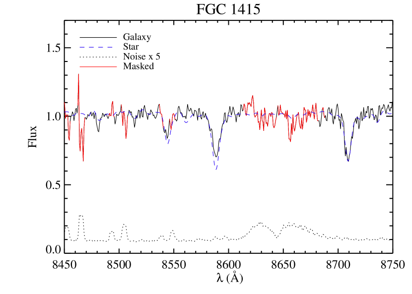
Figure 3.— An example of our extracted galaxy spectra. The solid line shows the normalized galaxy spectrum. Red regions mark where the spectra was masked due to sky line contamination. The noise spectrum (multiplied by 5) is plotted as a dotted line. The blue dashed line shows the best fit shifted and broadened stellar spectrum.

Because we have modified the traditional cross-correlation technique, we have no formal means of calculating uncertainties in our fitted velocity and LOSVD. We therefore run a series of Monte Carlo realizations to quantify the errors in our fitting procedure. For each galaxy, we create 100 artificial 2D spectra. A template stellar spectrum is shifted to match a realistic rotation curve, and broadened to simulate both stellar velocity dispersion and instrumental resolution. We vary the detailed shape of the rotation curve and velocity dispersion for each realization by $\sim 20$%. The fake spectra have radial exponential flux profiles similar to the real galaxies. We add Poisson noise to the artificial spectra, as well as systematic residuals by adding regions of sky from our science frames that do not have any detectable objects. Thus, our artificial spectra have both the same Gaussian sky background and similar systematic residuals as the real data.

Once the artificial spectra are made, we extract and analyze 1D spectra identically to the real data (i.e., we use the same extraction windows and the cross-correlation with masking procedure). In many instances, we found that our measured LOSVD poorly matched the input. The loss of reasonable LOSVD measurements is dominated by how many of the Caii lines are masked due to sky line contamination. We therefore clip points where the Monte Carlo error analysis suggests we cannot reliably recover the input parameters (i.e. the RMS error between input and output is $>50$ km s^-1 or the output has a systematic error of $>20$ km s^-1). These clipped regions typically correspond to regions of the rotation curve where the Ca triplet line passes through a large sky residual.

Our final extracted rotation curves, LOSVDs, and Monte Carlo derived uncertainties are plotted in Figure 4 along with $R$-band images of the galaxies showing the Gemini longslit placements.

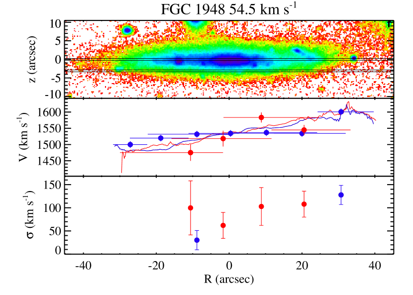
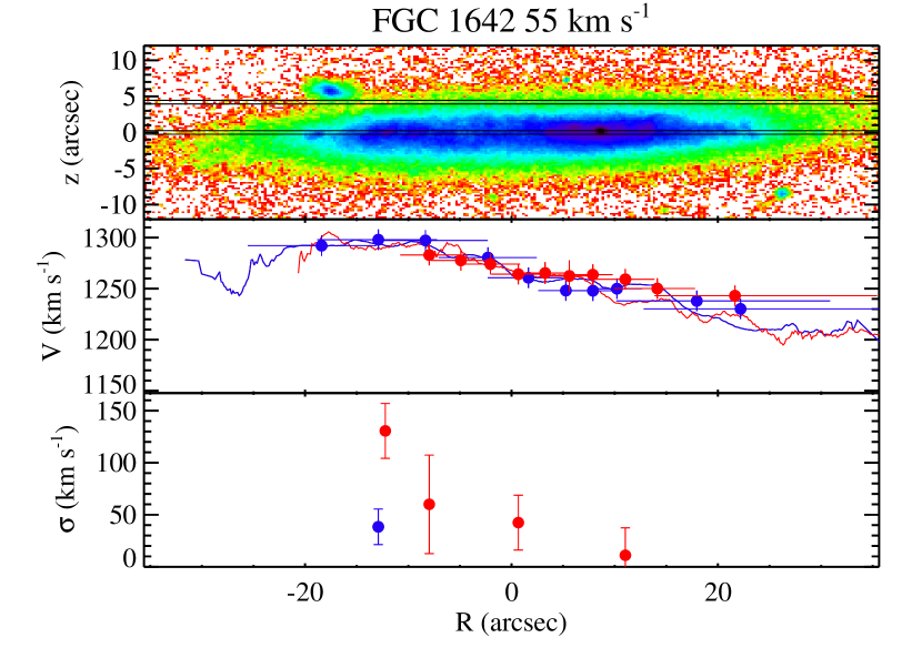
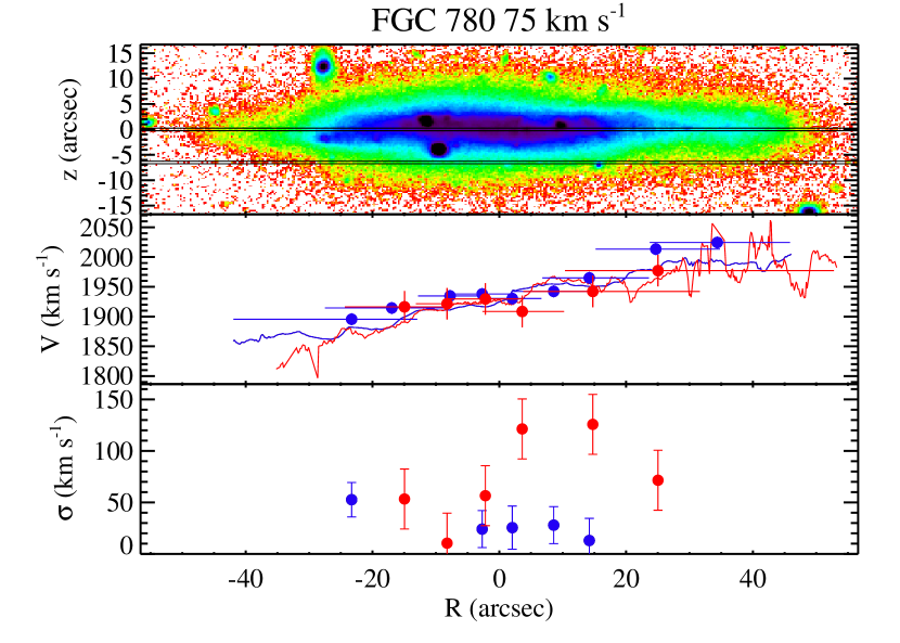
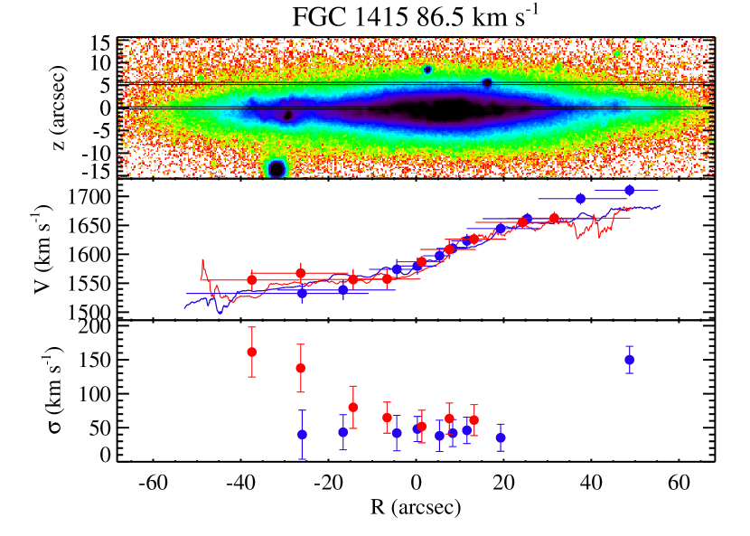
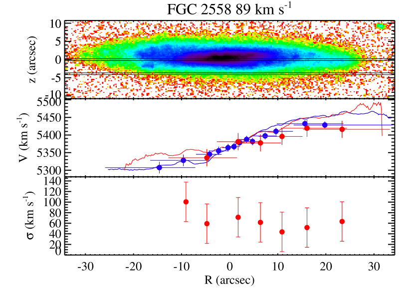
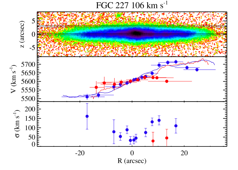
Figure 4.— Rotation curve measurements for each galaxy. Top panels: $R$-band images of each galaxy. The color scale goes from dark blue ($\mu_{R}=21$) to green($\mu_{R}=23$), to red/white ($\mu_{R}=25.5$). Solid black lines have been drawn where the Gemini long-slit jaws were placed. Middle Panels: Rotation curves for midplane (blue) and offplane (red). Points with error bars are from Ca ii measurements. Vertical error bars are uncertainties derived from Monte Carlo simulations, horizontal error bars show the spectral extraction regions. Small lines show velocities measured from the H$\alpha$ emission lines. Bottom Panels: Stellar velocity dispersions measured from the Ca ii feature. All error bars are from a Monte Carlo simulation. Points with overwhelmingly large error-bars or large systematic uncertainties have been omitted.

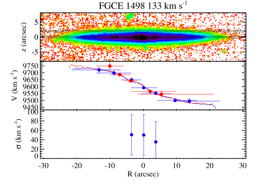
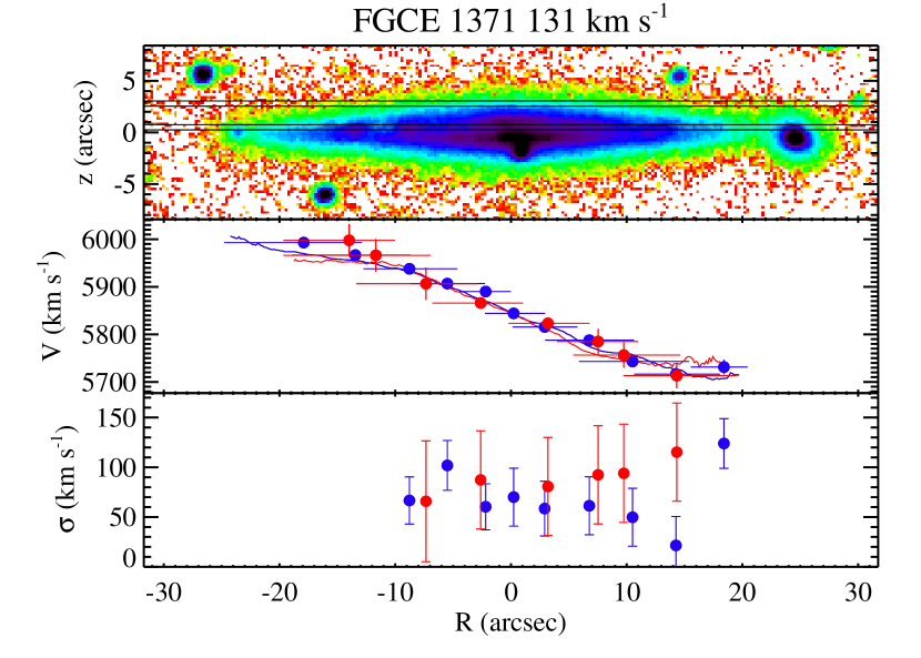
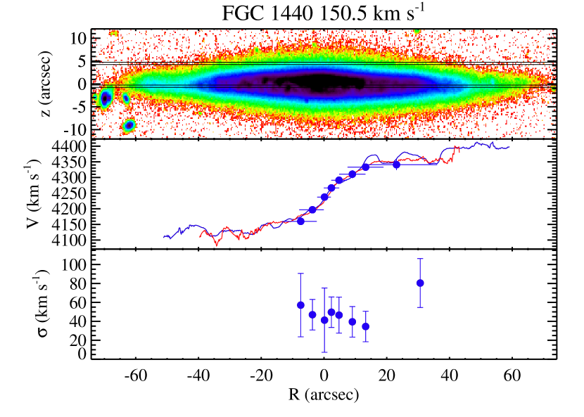
Figure 4.— continued.

4. Stellar Kinematics

Although we attempted to place our slits in regions of the galaxies where the thin and thick disk light makes up the majority of the flux, it is nearly impossible to target regions where one stellar component completely dominates the flux. In the lower-mass galaxies, we found that the thick disk is a major stellar component and we should expect spectra taken along the midplane to include a large amount of thick disk light. In the higher mass galaxies, the thin disk is the dominant component, and we are forced to observe off-plane regions that still contain a large fraction of thin disk light. Using the photometric fits of Yoachim & Dalcanton (2006), we can estimate the fractional flux levels of the thin and thick disk at each slit position. Because each slit position should include both thin and thick disk stars, we make an attempt to model the true underlying rotation curves for each population. For simplicity, we assume that the thin and thick disk stars are each rotating cylindrically and therefore have the same rotation curve for both the on and off-plane observations. We discuss this choice in more detail in §6.

The details of the vertical profiles of the stellar disks (exponential vs sech²) can dramatically influence what fraction of the midplane light belongs to thin disk stars versus thin disk stars. As in Yoachim & Dalcanton (2005), we adopt a series of photometric decomposition models that should cover the full range of possible thin and thick disk fractions. At one extreme, we use a simple model where we assume the midplane is composed of only thin disk light and the offplane observations purely thick disk stars. As a more accurate model, we use the thin/thick fractions from the best fitting models of Yoachim & Dalcanton (2005) as well as models where we vary the parameters by their 1-$\sigma$ values to create a “bright-thick and faint-thin” model along with a “faint-thick and bright-thin” model. The differences between the thin and thick disk scale lengths are small enough that we do not expect much radial variation in the fraction of thin and thick disk light.

In Yoachim & Dalcanton (2005), we fit analytic functions to the stellar rotation curves to decompose the thin and thick disk components. This worked well for the initial two galaxies we observed, but our expanded sample now includes galaxies with slightly irregular kinematics that are not well described by common parameterizations of rotation curves. Instead of using an analytic function, we use the midplane H$\alpha$ rotation curve as a basis function for the overall shape of the rotation curve. Because we are most interested in finding the velocity of the thin and thick disk stars relative to each other, we compare them both to the well resolved and high signal-to-noise midplane H$\alpha$ rotation curve. Using the $\rm{H}\alpha$ rotation curve reduces the number of parameters that need to be fit to characterize the stellar rotation curves.

We model the stellar rotation curves as $V_{stars}(R)=xV_{\rm{H}\alpha}(R)+c$. We constrain $c$ to be in the range $\pm 5$ (to account for any small error in wavelength calibration between frames or regions on the chip) and $x$ is limited to $-1<x<1.4$, allowing for stars to be rotating faster than the gas by up to 40% ($x$=1.4), not rotating ($x$=0), or counter-rotating with the opposite velocity of the H$\alpha$ ($x$=-1).

The decomposed rotation curves are plotted in Figure 6. The left hand panels show the best fit stellar rotation curve scaled from the $\rm{H}\alpha$ at each slit position. If there were no cross-contamination of thin and thick disk stars, then the offplane and midplane rotation curves would show the true thick and thin disk kinematics. The right hand panels show the more realistic case where we have adopted likely amounts of thin and thick disk contamination at each slit position before inferring the underlying kinematics of each population.

For the higher mass galaxies, we find no substantial difference between the thin and thick disk rotation curves, even when we correct for the expected cross contamination. There is a slight tendency for the thick component to be lagging, but never by more than 5 km s^-1. In the higher mass galaxies, we have therefore either failed to observe an offplane region with a high enough thick disk flux fraction, or the thick disks are not lagging significantly compared to the thin disk in these systems.

For the low-mass galaxies, we find a wide range of behavior. The fits for FGC 1948 diverge, as the stellar rotation curves do not show coherent rotation at either slit position. For the rest of the galaxies, the best fits find thick disks that are slightly lagging compared to the thin (FGC 2558, FGC 1415), that are lagging to the extent of near non-rotation (FGC 1642, FGC 780), and that are fully counter-rotating (FGC 227). We note that there is strong qualitative agreement with initial results in Yoachim & Dalcanton (2005) for FGC 1415 and FGC 227.

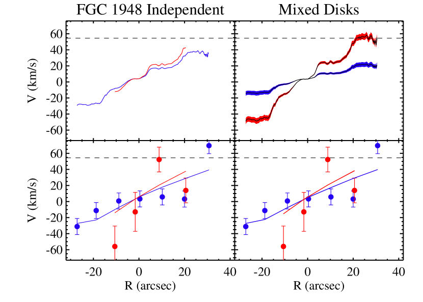
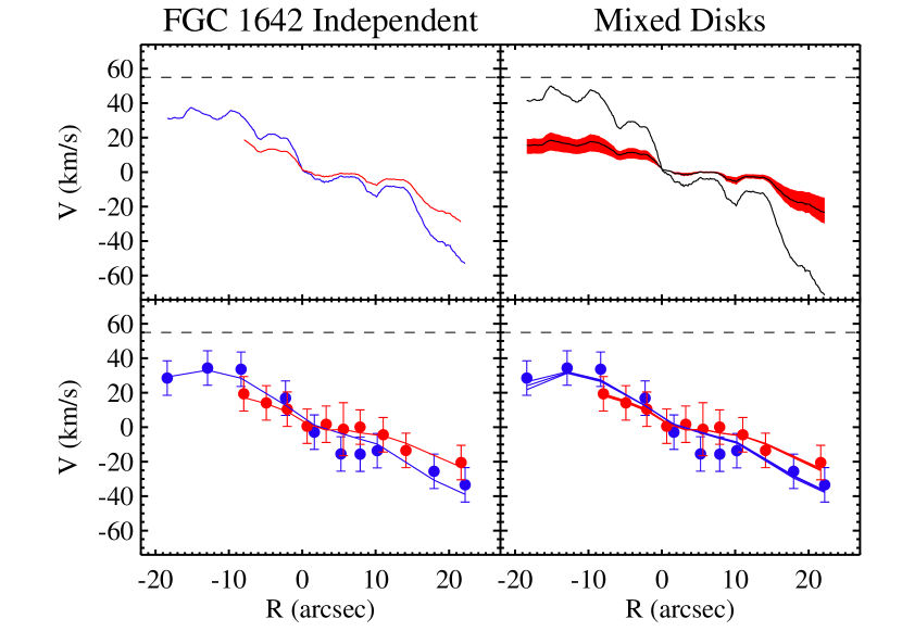
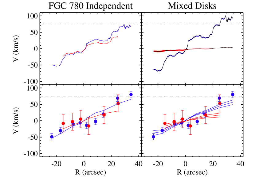
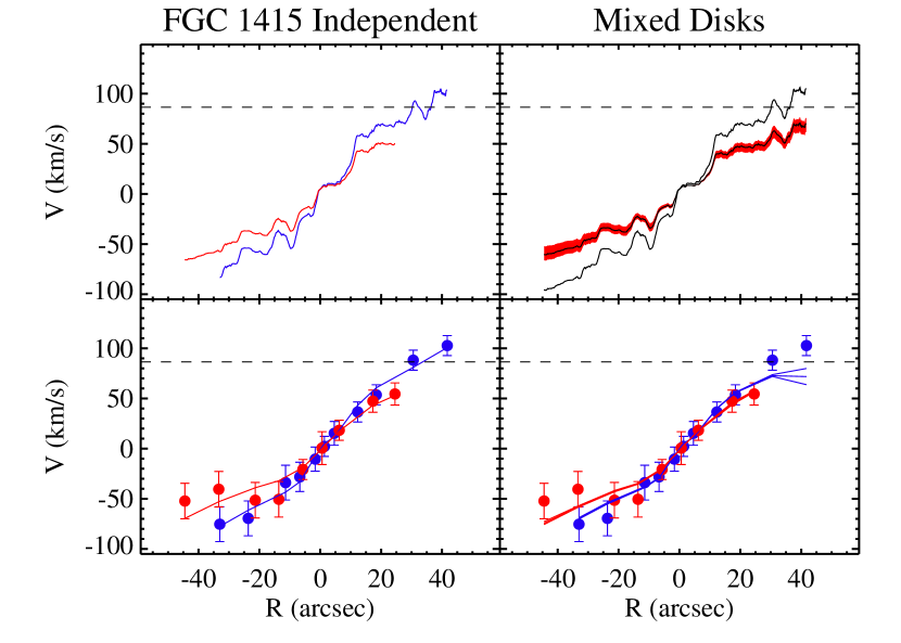
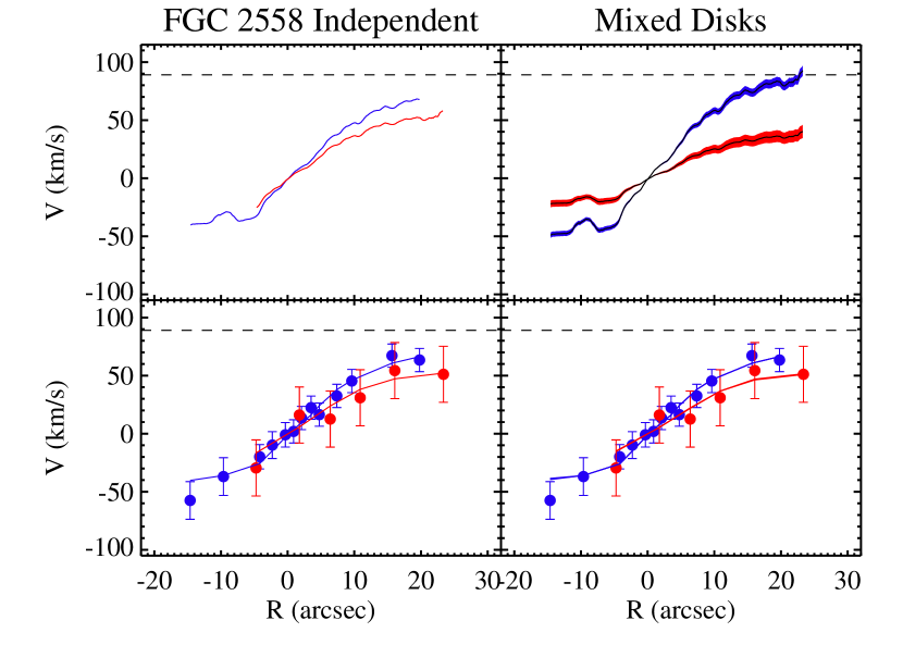
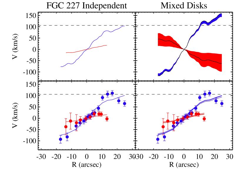
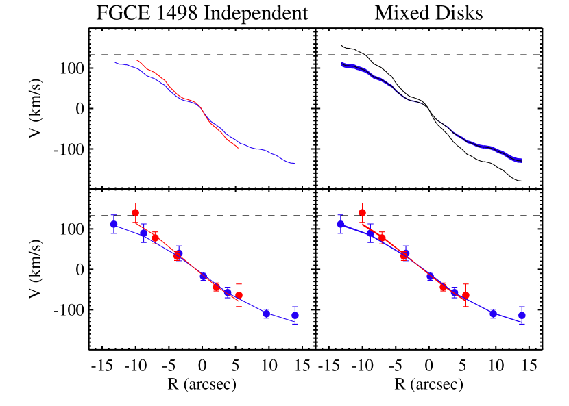
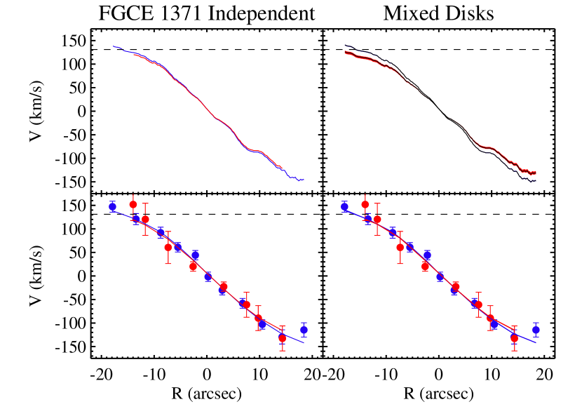
Figure 6.— The results of fitting various rotation curve models to our data. The top left panels show fits of the simple model where the midplane and offplane observations are fit independently. Upper right panels show shaded regions show the range of fits derived from varying the fraction of thin and thick disk light at each slit position. Solid lines show the fits for when we use the thin and thick disk fractions of the photometric fits in Yoachim & Dalcanton (2006). Lower panels show the observations as points and solid lines show the models from the above panels once they have been flux weighted and binned in the same manner as the observations. Throughout, red is used for thick disk/offplane and blue is used for thin disk/midplane. Each panel has a dashed line showing the W50/2 value from the literature. FGC 1440 is not shown because we failed to measure a stellar rotation curve in the offplane position.

4.1. Velocity Dispersions

The low signal-to-noise of our spectra prevents us from reliably measuring velocity dispersions for many of our galaxies. Most of the galaxies with high quality spectra have very low velocity dispersions, as we would expect from systems predominantly supported by rotation. Given that our instrumental resolution is 60 km s^-1, we are unlikely to resolve the line widths in galaxies where $\sigma/V_{c}<0.6$, for the $V_{c}<100$ km s^-1 galaxies that dominate our sample. The major exceptions are FGC 1948, which has an irregular rotation curve, and FGC 227, which has a counter-rotating thick disk.

FGC 1948 has surprisingly large LOSVD, with many regions of the disk having $\sigma>100$ km s^-1. For comparison, most of the other galaxies in our sample have LOSVDs across the disk of $\sim 50$ km s^-1, essentially the same as our instrumental resolution at the Ca ii triplet. The stellar rotation curve for FGC 1948 also shows large deviation from the H$\alpha$ RC, suggesting that the stars in this galaxy might not be fully rotationally supported and/or fully dynamically relaxed.

FGC 227’s LOSVD also deviates from the simple interpretation of a dynamically cold rotating disk. In the midplane observations, the central regions of FGC 227 appear cold ($\sigma\sim 40$ km s^-1), but the outer disk reaches LOSVD values of 100-150 km s^-1. This makes little sense for a galaxy with a well defined rotation curve as the intrinsic stellar velocity dispersions should be decreasing with radius. In contrast, the LOSVD can be well explained by a rotationally supported galaxy if there are two stellar populations moving in opposite rotational directions. As our rotation curve decomposition showed, FGC 227 is best fit by a model where the thick disk is counter-rotating relative to the thin disk. As we showed in Yoachim & Dalcanton (2005), this would cause an increase in the observed velocity dispersion of order 50 km s^-1. Similar projection effects are found in elliptical galaxies with counter-rotating cores as they also show radially increasing LOSVDs (Geha et al., 2005).

5. How Much Counter Rotating Material Could There Be?

Inspired by the best-fit rotation curve for FGC 227, we investigate the possibility that all thick disks contain some fraction of counter-rotating stars. Our data is able to place tight constraints on the amount of counter-rotating material since both the offplane rotation curves and the midplane LOSVD will be strongly affected by any counter-rotating stars.

In Section 4, we imposed thin and thick disk flux fractions based on previous photometric decompositions. We now leave the flux fractions as free parameters and instead hold the rotation curve shapes fixed. We fit two simple models, each with two kinematically independent stellar components. In the first model, we assume there are two stellar components, one rotating identically as the gas and one with zero net rotation, as one might expect for a stellar halo. The final observed rotation curve is a flux weighted average of these two curves and we fit for the best fitting flux ratio. We restricted the explored parameter space such that the rotation curves had to be some positive linear combination of the midplane H$\alpha$ and a non-rotating or counter-rotating rotation curve. In the second model, we assume the second component is counter-rotating with a velocity one-half the magnitude of the H$\alpha$ rotation curve. For both models, we calculate uncertainties from the covariance matrix and scale them upwards such that the reduced-$\chi^{2}$ equals unity (i.e., we assume our model should be a good fit). We do not calculate uncertainties when the fit converges to a boundary condition. We also do not construct detailed models for cases like FGC 1415 where the stars could be better fit with a faster rotation curve than the gas; these galaxies naturally converge on the boundary condition of having no second component. It should be emphasized that these are simple toy models, and we have no direct evidence of counter rotating thick disk stars beyond the strange rotation curve of FGC 270. For example, if we observed a MW like (V${}_{\rm{c}}=220$ km s^-1) galaxy that had a 10% (by flux) thick disk lagging at 40 km s^-1, we would compute a maximum counter-rotating fraction of 1% and a non-rotating fraction of 2%, despite all the stars being co-rotators.

The resulting fractions of non-rotating of counter rotating stars are plotted in Figure 7 and are listed in Table 4. The midplane stellar rotation curves are typically consistent with the H$\alpha$ rotation curve, with 6 of the 9 midplanes being best fit without a non-rotating or counter-rotating component. The remaining three galaxies do have midplane rotation curves that are consistent with the presence of an additional lagging component. FGC 1948 is low mass with a surprisingly large LOSVD. FGC 227 is the counter rotator with a LOSVD that dramatically increases with radius. FGC 2558 is the only galaxy to show a large discrepancy between midplane and offplane H$\alpha$ rotation curves, has a stellar lag that appears to be only on the receding side of the galaxy.

The offplane spectra show larger evidence for non- or counter-rotating motion, with only 3 of the 9 galaxies requiring no slow rotating component. This effect can be seen in Figure 7, where all of the offplane spectra show a preference for equal or larger value of the counter-rotating fraction than seen in the midplane.

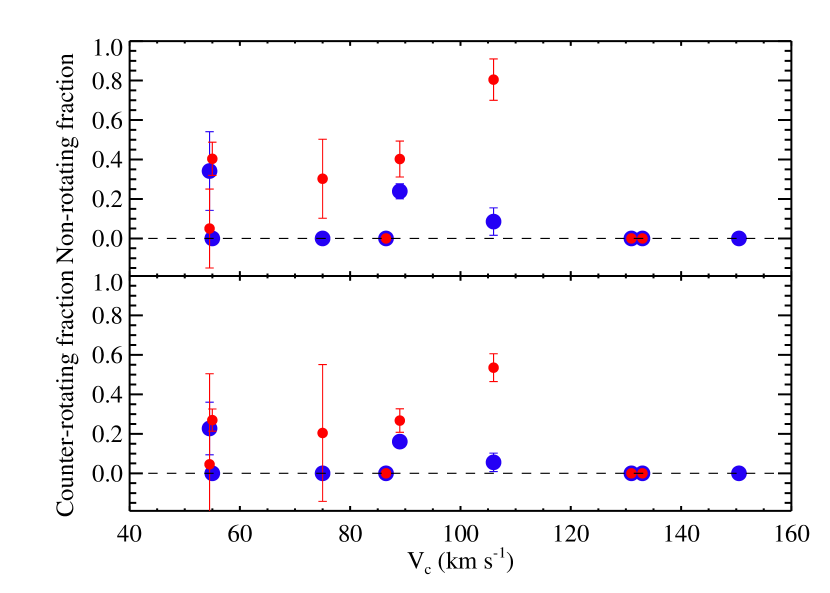
Figure 7.— Results from fitting the midplane and offplane rotation curves as a combination of two fixed rotation curves. In the top panel, the rotation curves are a combination of the midplane H$\alpha$ and a flat non-rotating RC. In the bottom panel, the base rotation curves are the midplane H$\alpha$ combined with a rotation curve counter-rotating with one-half the H$\alpha$ velocity. These fits are listed in Table 4.

Table 4Non-Rotating and Counter Rotating Fractions

FGC	Non-Rotating Fraction		Counter-Rotating Fraction
	Thin Disk	Thick Disk	Thin Disk	Thick Disk
227	0.1$\pm$ 0.1	0.8$\pm$ 0.1	0.1$\pm$ 0.0	0.5$\pm$ 0.1
780	0.0	0.3$\pm$ 0.2	0.0	0.2$\pm$ 0.3
1415	0.0	0.0	0.0	0.0
1440	0.0	$\cdots$	0.0	$\cdots$
1642	0.0	0.4$\pm$ 0.1	0.0	0.3$\pm$ 0.1
1948	0.3$\pm$ 0.2	0.1$\pm$ 0.2	0.2$\pm$ 0.1	0.0$\pm$ 0.5
2558	0.2$\pm$ 0.0	0.4$\pm$ 0.1	0.2$\pm$ 0.0	0.3$\pm$ 0.1
E1371	0.0	0.0	0.0	0.0
E1498	0.0	0.0	0.0	0.0

6. Expected Lags

Having found a wide range of thick disk behaviors, we now investigate the expected stellar lags we should see in our sample of thick disks using a dynamical model originally designed for the Milky Way. The large scale height of thick disk stars implies they have larger velocity dispersions than thin disk stars. If the larger vertical velocity dispersion also reflects a larger radial velocity dispersion, then the larger random motions of thick disk stars should lead to their requiring less rotational support. The thick disk stars should therefore lag in velocity compared to the kinematically colder thin disk stars and ionized gas.

Girard et al. (2006) use the Jeans equation and a series of reasonable assumptions to model the expected thick disk lag in the MW as a function of height above the midplane. While this model was built to explain the observed lag of thick disk stars in the Milky Way, the formalism is easily generalizable to the galaxies in our sample.

Using the Jean’s equation, Girard et al. (2006) find that the rotational velocity of a thick disk rotating in a Plummer dark matter potential with an embedded thin disk is given by:

$${\overline{v_{\Theta}}}^{2}(z,R)=\sigma_{R}^{2}(z)\Big{[}-{\Upsilon_{a,b}R}$$ (1)

$$+0.5\lambda\Big{(}1-{z\over h_{z_{thick}}}\Big{)}+1-{\sigma_{\Theta}^{2}\over\sigma_{R}^{2}}\Big{]}$$

$$+{(v_{c}^{2}-v^{2}_{disk}(R,0))(R^{2}+a^{2})^{3/2}\over(R^{2}+z^{2}+a^{2})^{3/2}}+v^{2}_{disk}(R,z),$$

where $R$, $z$, and $\Theta$ are galactocentric cylindrical coordinates. The term ${\overline{v_{\Theta}}}$ is the average thick disk velocity in the direction of galactic rotation, $\sigma_{R}$ and $\sigma_{\Theta}$ are the radial and tangential components of velocity dispersion for the thick disk stars, $v_{c}$ is the local standard of rest velocity at the radius of interest, $v_{disk}$ is the portion of the thick disk rotational velocity due to the gravitational potential of the thin disk, $h_{z_{thick}}$ is the exponential thick disk scale height and $a$ is the halo core radius. The term $\Upsilon_{a,b}$ lets one approximate the thick disk as entirely self gravitating, or gravitationally dominated by the embedded thin disk. Because the thick disk mass is small compared to the total gas and thin disk mass in all of our galaxies, we choose to use $\Upsilon_{b}\sim 2/h_{R}$. The $\lambda$ term takes values of 1 or 0 in order to include or exclude the velocity dispersion cross-term.

We calculate dynamical models for three fiducial galaxy masses and three thick disk velocity dispersions. We use realistic galactic parameters taken from Yoachim & Dalcanton (2006) to generate $h_{z_{thick}}$ and $v^{2}_{disk}(R,0)$. For terms for which we do not have explicit measurements, we use the approximation $a[\rm{kpc}]\approx 13(h_{r_{thin}}[\rm{kpc}]/5)^{1.05}$ given by Donato et al. (2004), assume $\sigma_{\Theta}\sim\sigma_{R}$, and set $\lambda=0$. We compute models for different values of $\sigma_{R}$, as this is the dominant term in producing stellar lags. For simplicity, we assume the thick disk velocity dispersion does not vary with height above the midplane. This last approximation is not particularly valid given that Girard et al. (2006) find that the velocity dispersion in the MW increases with a slope of 9 km s^-1kpc^-1. However the difference between a variable and constant velocity dispersion will be most pronounced at large scale heights, beyond the range probed by our observations ($z\sim 1.5-2$ kpc). The resulting models are plotted in Figure 8 along with the lags we have measured in our galaxies. For reference, we also include a model using the same assumptions but with morphology and velocities similar to the Milky Way in Figure 8.

For most of the galaxies where we measure a thick disk lag, Figure 8 shows the thick disk kinematics could be well explained by a population with radial velocity dispersion of between 15 and 30 km s^-1and $v_{c}/\sigma<4$. As before, the major exception is FGC 227. The stellar lag for FGC 227 is so severe that it would imply the thick disk is completely supported by random motions. However, we only detect flattened stellar populations in FGC 227, again consistent with our interpretation that the thick disk is counter-rotating in this system.

To verify that our model galaxies are reasonable, we use an identical procedure to build a MW-like model. Our MW-like model is a fair fit to actual observations of the MW. The measured thick disk velocity dispersion in the solar neighborhood is 50 km s^-1, for which our model correctly predicts the midplane thick disk lag of 30 km s^-1. On the other hand, the increase of the thick disk lag with scale height is poorly fit by our model; the observed lag increases with a slope of 30 km s^-1kpc^-1, and our model has a slope around half that. This is purely due to our choice to hold the velocity dispersion fixed–a thick disk velocity dispersion that increased with height would generate a more accurate slope.

Figure 8.— The expected thick disk lags as a function of height above the midplane and thick disk velocity dispersion. The first three panels show model galaxies similar to the ones in our sample. Points show the stellar lags measured from our rotation curve fits. Open points show lags from rotation curves where the offplane and midplane rotation curves are fit independently. Solid points show the average lag for the models which correct for cross-contamination of the thin and thick disk rotation curves, and are generally more reliable estimates of the thick disk lag. The final panel shows the results of our model when we use MW like parameters. Observed galaxies we compare to the models: In the upper left FGC 1642 and FGC 780; upper right FGC 1415, FGC 227, and FGC 2558; and lower left FGCE 1371. All the models and observations are taken at $R=2.5h_{R}$. FGC 1948 is excluded from the plot because there is no coherent rotation. FGC 1440 is excluded because we have no offplane stellar velocity measurements.

Modeling the disks as cylindrically rotating is only a crude approximation to account for the stellar cross-contamination. In reality, we expect the thin disk stars which reach large $z$ heights to be the thin disk stars with larger velocity dispersions. This would mean that the thin disk stars at high $z$ should also be lagging compared to the midplane thin disk stars. Ideally, we would construct a fully self-consistent dynamical model of each galaxy, but our large uncertainties and limited LOSVD information would result in model degeneracies. Constructing a robust self consistent dynamical model of a galaxy also benefits from larger numbers of data points (Girard et al., 2006). With only a handful of stellar rotation curve points per galaxy, we do not have enough data to constrain a more complex model. We simply point out that when we correct for the cross-contamination of the rotation curves we may be over-correcting the data. We estimate the magnitude of the over-correction using dynamical models in § 6.

7. Dust and Projection Effects

As a final check that our observed kinematics indeed reflect the true stellar motions, we now explore the expected impact of projection effects and dust extinction, both of which can create differences between the observed and underlying rotation curves. In Figure 9, we show how two input rotation curves are modified by being viewed edge-on, with and without dust. For these models, we assumed an exponential disk of stars and dust, and for simplicity only considered absorption (i.e., ignoring scattering). The amount of dust adopted in the model would generate an extinction of 2.2 magnitudes in the total apparent magnitude of the galaxy. This is a rather large extinction for the near-IR, given that the observed galaxies in our sample are only offset by 0.2 mag from the face-on NIR Tully-Fisher relation (Yoachim & Dalcanton, 2006). We adopted an underlying rotation curve shape from Courteau (1997).

As can be seen from Figure 9, the inner regions of the rotation curve are generally unchanged due to projection, and the only significant changes happen in the outer regions, where the true rotation curve is flat. These projection effects create a lag of 7.2 km s^-1.

We have not corrected our rotation curves for these projection effects, as we are primarily interested in the differences between the thin and thick disk rotation curves. This could lead us to make systematic errors in interpreting the rotation curves if the morphologies of the thin and thick disk are radically different, but we have no reason to assume this is the case.

When dust is added to the model, it only creates an additional 2.6 km s^-1 lag, in spite of the very high extinction adopted here. This model is completely consistent with the results of Matthews & Wood (2001), who found that projection effects are dominant compared to extinction in edge-on systems. We do not expect our sample galaxies to have larger extinctions than what is modeled in Figure 9.

Full radiative transfer models (Kregel & van der Kruit, 2005; Bianchi, 2007; Xilouris et al., 1999), as well as comparisons of gaseous and optical rotation curves (Bosma et al., 1992) have consistently found massive disk galaxies have a central face-on optical depth near unity in the $V$-band, with lower extinction levels in less massive systems like those that dominate our sample (Calzetti, 2001). Dust levels this low should not be expected to alter the observed rotation curve significantly, even if a galaxy is viewed edge-on. Moreover, most of our offplane rotation curves exhibit a lag compared to the midplane. In contrast, If there were strong dustlanes affecting our midplane observations (and not the offplane), the midplane would be the lagging component.

The combination of working at near-IR wavelengths, offsetting our slit from any prominent dustlanes, and observing intrinsically linearly rising rotation curves means our rotation curves should be fairly unaffected by extinction or projection. However, the same cannot be said for our measured line-of-sight velocity dispersion (LOSVD). Unlike the rotational velocity measurement, which is mostly unaffected by flux contributions from different radii, we expect the LOSVD to be significantly broadened by projection effects. We also find that in most of our galaxies the LOSVD is very close to the instrumental resolution, making any interpretation of the velocity dispersion suspect. Because of these challenges, we limit our analysis of the LOSVD to only those cases where we believe our measurements are of high quality and not dominated by the instrumental dispersion.

Figure 9.— Two examples of the effects dust and projection can have on our observed rotation curves. While projection creates considerable changes, the addition of dust extinction is negligible.

8. Discussion

The results of Sections 3.2 and 4 show that stellar kinematics above the midplane display a wide range of behaviors. In higher mass systems (FGCE 1371, FGCE 1498, FGC 1440), our midplane and offplane spectra show no clear signature of a hot thick disk component. The stellar rotation curves for these galaxies are well matched by the midplane ionized gas H$\alpha$ RCs at all measured scale heights. All three of these galaxies converged to models where the rotation curves contain no lagging component (Table 4). However, Yoachim & Dalcanton (2006) found that the stellar flux in higher mass galaxies are dominated by the thin disk component. Therefore, the lack of a significant lag in these systems is likely a result of the kinematically cold thin disk dominating the stellar flux to scale heights of 1 kpc. This result is not completely unexpected, as the MW thin and thick disks should have similar luminosities 1 kpc off the midplane (Jurić et al., 2008). We note that there is still ample photometric evidence that these higher mass galaxies contain thick disks, but they are simply too faint relative to the thin disk for modest kinematic lags to be detected spectroscopically.

The low mass galaxies in our sample do show measurable differences between the midplane and offplane observations. At large radii, we find several galaxies where the offplane component is lagging compared to the midplane (Figure 8). In three of the low mass systems (FGC 1415, FGC 1642, and FGC 780), the lags in the offplane observations become more pronounced when we correct for the expected thin disk contamination. These lags are consistent with those that are expected from dynamics alone (Equation 1), provided that the thick disk has a radial velocity dispersion between 15 and 30 km s^-1(i.e., 10-25% of $v_{c}$). Thus, the lags in these systems do not necessarily require the presence of any counter-rotating material, although a small amount of such material could be present. FGC 2558 may also fall into this category; however the offplane RC is very similar to the midplane, implying this could be another galaxy where we have not successfully isolated the thick disk. The observed lags were easier to detect in these lower mass systems, due to their more prominent thick disks.

The final two low mass galaxies in our sample, FGC 227 and FGC 1948, have remarkably different rotation curves between the midplane and offplane. FGC 1948 does not display coherent stellar rotation in either the midplane or the offplane, and therefore our subsequent fits converge to extreme, and probably incorrect, models. FGC 227 does show rotation on the midplane, and a very low level of net rotation on the offplane. Our best fitting model for this galaxy has the thick disk counter-rotating relative to the thin disk, consistent with the radially increasing LOSVD which is a signature of unresolved counter rotating stellar components.

Our measurements of the LOSVD are less than enlightening. With the exception of the radial increase in the LOSVD in FGC 227 and the high LOSVD in FGC 1948, the rest of our LOSVD measurements show no significant trends with radius and are close to the instrumental resolution limit, suggesting that the radial velocity dispersions of both the thin and thick disks are cold enough that we cannot reliably measure their velocity dispersions at our spectral resolution.

Given the above results, our galaxies can be described as falling into three categories: The high mass systems which have little to no thick disk lag (or, more likely, thick disks which are so faint that we have failed to measure their kinematics); the moderately lagging systems; and the counter rotating system. We can now compare these results to the predictions of popular formation models for the thick disk.

If thick disks are the result of gradual stochastic heating, we would expect to always find thick disks co-rotating with the embedded thin disks. Moreover, with stronger spiral arms, larger molecular clouds, and more massive dark matter substructure, the high mass systems should be able to efficiently heat their thin disk stars into a thicker disk. Instead, we have found the opposite, with more prominent thick disks and larger lags in the lower mass systems, as well as evidence for counter-rotating stars. This seems to rule out gradual heating as the dominant method of thick disk formation, particularly for low mass galaxies.

Forming thick disks in major mergers also does a poor job explaining our observations. If thick disks were predominantly formed in major mergers that disrupt and heat previously thin disks, we should expect to find galaxies that never formed a thick disk, or that have failed to accrete and cool enough gas to rebuild their thin disk components. Major mergers also typically result in the formation of centrally concentrated spheroidal components, making them a poor mechanism for forming thick disks in the bulgeless galaxies observed here.

Unlike the two heating models, the variety of thick disk kinematics is compatible with minor mergers and/or accretion. Presumably, the thick disk kinematics we observe are simply the kinematics left over from the accretion event which deposited the majority of thick disk stars or which triggered the formation of stars from gas accreted at large scale heights. The wide variety of possible accretion events (co-rotating vs counter rotating, early disruption vs late disruption, high eccentricity vs circular initial orbit) can evolve into virialized thick disks with kinematics that are sometimes decoupled from the thin disks and that show large variation from galaxy to galaxy. The ubiquity of thick disks is also well explained by the merger/accretion scenario, given that galaxy formation in a $\Lambda$CDM cosmology is dominated by hierarchical merging, and predicts that every galaxy has a rich merger history.

Although the available data all points to a merger/accretion origin for the thick disk, it is difficult to disentangle models where thick disk stars are directly accreted from those where the stars form in situ further off the midplane during gas rich mergers (Brook et al., 2004).

This ambiguity results from two sources. First, there is no clear dividing line between what one calls a star-forming region off the midplane and a merging star-forming satellite galaxy. Second, we know from Yoachim & Dalcanton (2006) that at least 75-90% of the baryonic accretion onto the galaxies was gaseous, and some fraction of this was certainly accreted in bound subhalos. Stars that formed initially in subhalos before being accreted are likely to have kinematics similar to those that formed from accreted gas during those same merging events. Presumably, one could use detailed stellar age and abundance information to help, but unfortunately this is only possible for the closest galaxies.

There is evidence that much of the brighter inner halo and outer disk substructure of M31 was formed through accretion (Ferguson et al., 2002; Koch et al., 2007). These features would probably resemble a thick disk if M31 were more distant and the features were unresolved. Taking this lesson from nearby galaxies, it is clear we are using smooth functions to describe thick disk that may actually be highly structured systems. However, the smooth descriptions of thick disks still provide a reasonable statistical description of the ensemble of accreted stars.

In this study, we have measured thick disk kinematics in only very late-type disk systems. However, thick disks have been photometrically detected in a wide variety of Hubble types (e.g., Seth et al., 2005; Pohlen et al., 2004; Morrison et al., 1997; van Dokkum et al., 1994). The kinematics in our sample are most consistent with merger/accretion forming for the thick disks, but, except for the Milky Way, there have been no measurements of thick disk kinematics in earlier type galaxies.

By focusing on disk systems, we may not be sensitive to how thick disks form across all Hubble types. Almost by definition, late-type galaxies have not suffered a major-merger since the formation of their stellar disks, otherwise they would likely possess large spheroidal components and be classified as an earlier type system. The only way pure disk galaxies could form thick disks is either through accretion or stochastic heating.

9. Conclusions

We have expanded the kinematic observations of Yoachim & Dalcanton (2005) to include a total of nine galaxies with thick disks. Analyzing our low signal-to-noise spectra that contain systematic sky line residuals prompted us to develop a brute-force method of cross-correlation to extract stellar rotation curves. In galaxies with $V_{c}>120$ km s^-1, we do not detect any measurable difference between the thin and thick disk stellar kinematics. This is most likely due to a combination of thin disks being brighter in more massive galaxies, and the expected change in rotation curve as a function of scale height being smaller.

In lower mass galaxies ($V_{c}<120$ km s^-1), we find a variety of thick disk behaviors. Thick disks are found with both small and large magnitude lags, including a counter-rotating thick disk.

The observed kinematics are best explained by thick disk formation models where the thick disks in low mass systems are composed of stars that have been accreted from satellite galaxies or are formed at large scale heights from accreting gas. Models where the thick disks form during major mergers or through stochastic heating seems unable to explain the wide range of thick disk kinematics we observe. While we strongly favor a formation model of thick disks via accretion, we stress that this result can not necessarily be generalized to other Hubble types or higher mass systems ($V_{c}>120$ km s^-1).

Appendix A Stellar Rotation Curves in the Presence of Systematic Errors

Working in the near-IR, we find our spectra have regions which are dominated by both Gaussian and systematic errors caused by bright atmospheric emission lines. To properly measure stellar kinematics based on spectral absorption features we must employ a method that is not affected by our sky line residuals.

There are two common techniques of deriving the kinematic information from galaxy spectra–direct $\chi^{2}$-fitting and cross-correlation. In direct $\chi^{2}$-fitting (Rix & White, 1992; Kelson et al., 2000; Barth et al., 2002; Cappellari & Emsellem, 2004), a template star is redshifted and broadened to fit a galaxy spectrum, while in cross-correlation techniques (Simkin, 1974; Tonry & Davis, 1979; Statler, 1995) a template star is cross-correlated with the galaxy spectrum and the kinematic properties are deduced from the position and shape of the cross-correlation peak.

Cross-correlation techniques have the advantage of being computationally efficient, often making use of fast Fourier transform algorithms. The cross-correlation technique benefits greatly from the fact that the Fourier transform of Gaussian noise is also Gaussian noise. In this way, noise in the galaxy spectrum transforms into random noise in the cross-correlation while the kinematic information becomes concentrated in a central peak. However, this is only true if the noise is uniform throughout the spectrum. Using a direct chi-squared fit is more computationally expensive, but has the added benefit of being able to weight individual wavelengths according to their specific signal-to-noise, or completely mask wavelengths that are affected by systematic errors.

Although direct chi-squared fitting works well in some situations, at low S/N($<$20), any direct chi-squared fitting routine will over-smooth the data because the low S/N continuum is best fit by a strait line (i.e., an over-broadened template star). In previous studies that have used direct fitting, Kelson et al. (2000) has a median S/N of 35/Å, while Barth et al. (2002) report a S/N/pixel of 100-200. In contrast, our data has SNR$<20$/Å, due to the very low surface brightness of our targets.

Because we have both low S/N and regions which require masking, we have created a fitting procedure which utilizes cross-correlation without making use of the computational time saving FFT techniques of previous authors.

Traditional cross-correlation of discrete functions is defined as

$$(f\star g)_{i}\equiv\sum_{j}f_{j}g_{i+j}.$$ (A1)

We adopt a normalized version, where the means of the spectra have been subtracted before the cross-correlation is computed

$$(f\star g)_{L}=\frac{\sum_{k=1}^{N-L}f_{L}g_{k+L}}{\sqrt{\sum_{k=1}^{N}(f_{k})^{2}\sum_{k=1}^{N}(g_{k})^{2}}},$$ (A2)

where N is the number of points in the given spectra. For lags less than zero, the numerator becomes $\sum_{k=1}^{N-|L|}f_{k+|L|}g_{k}$. This ensures spectra with perfectly matching shapes will have a maximum cross-correlation amplitude of unity.

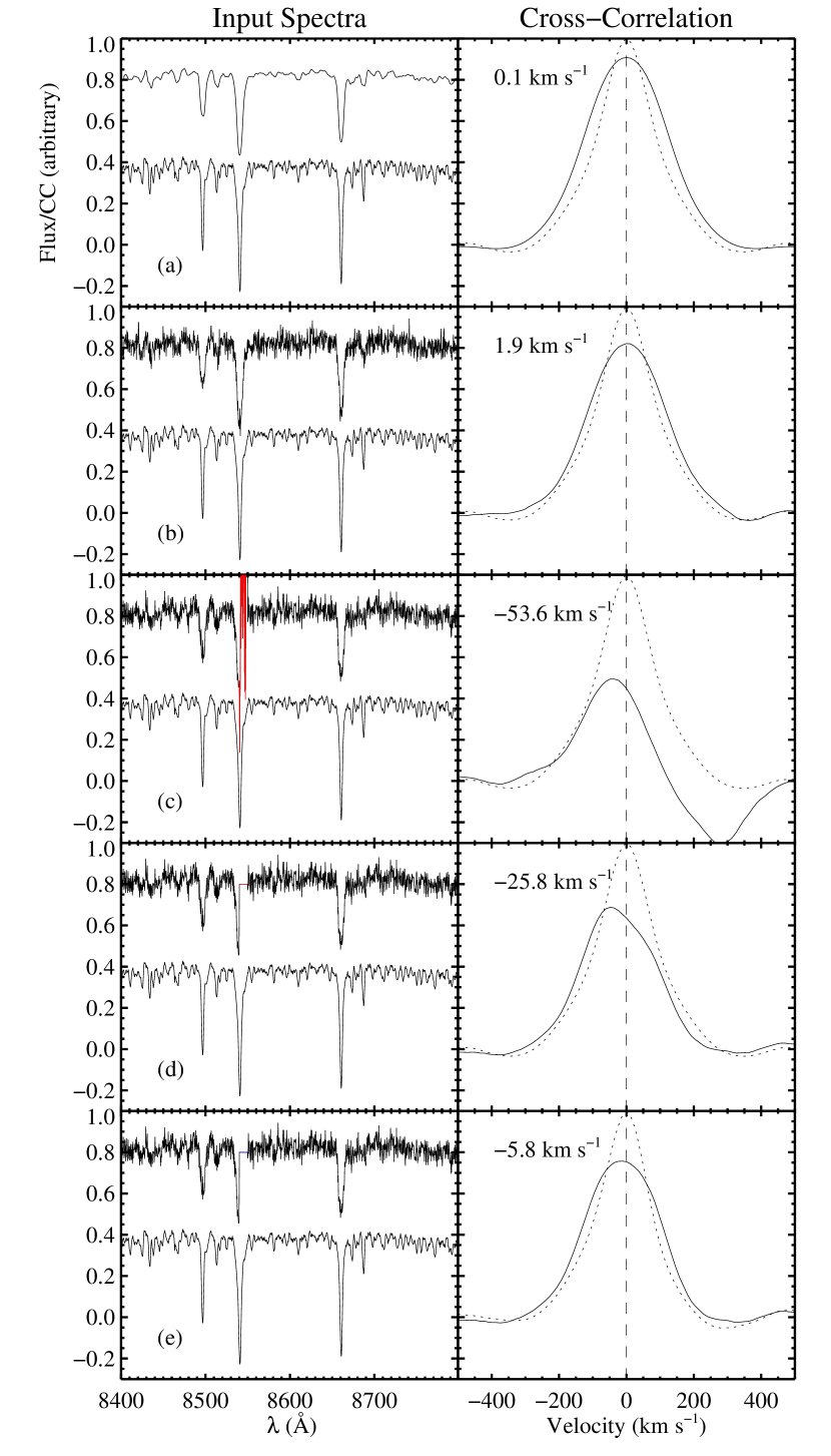
Figure 10.— Examples of cross-correlating in the presence of different types of noise. In the left hand column, we show a model galaxy spectrum (top) and stellar template (bottom). In the right hand column, we plot the galaxy-star cross-correlation (solid) and stellar auto-correlation (dotted) and note the velocity error resulting from comparing the two. (a) The ideal case of a high signal-to-noise galaxy spectrum. (b) Results from a galaxy spectrum with a S/N/Å$\sim 10$. (c) Spectra with a small region of very low S/N affecting a section of one of the Ca absorption features, similar to how bright sky lines leave residuals on our spectra. (d) A traditional cross-correlation where the noisy region has been set to the continuum. (e) Our new cross-correlation technique where we compute the cross-correlation excluding the masked region.

Finally, we define masks $\delta$ for each spectrum which have values of 1 in regions of good data and 0 for masked wavelengths. Given a stellar spectrum $S$ and Galaxy spectrum $G$ that are binned in logarithmic wavelength intervals and have both been normalized by division of a low order polynomial and had their means subtracted, we compute our modified cross-correlation as

$$(S\star G)_{L}=\frac{\sum_{k=1}^{N-L}S_{L}G_{k+L}\delta^{S}_{L}\delta^{G}_{K+L}}{\sqrt{\sum_{k=1}^{N}(S_{k}\delta^{S}_{K}\delta^{G}_{K})^{2}\sum_{k=1}^{N}(G_{k}\delta^{S}_{K}\delta^{G}_{K})^{2}}}.$$ (A3)

We then generate a model galaxy spectrum $M$ by redshifting and broadening the stellar template, $M(x)=S(x+v)\otimes B(x)$ where $B(x)$ is a Gaussian broadening function, $v$ is a velocity shift, and $\otimes$ represents convolution. We then calculate the model’s modified cross-correlation using the masks from the actual galaxy spectrum

$$(S\star M)_{L}=\frac{\sum_{k=1}^{N-L}S_{L}M_{k+L}\delta^{S}_{L}\delta^{G}_{K+L}}{\sqrt{\sum_{k=1}^{N}(S_{k}\delta^{S}_{K}\delta^{G}_{K})^{2}\sum_{k=1}^{N}(M_{k}\delta^{S}_{K}\delta^{G}_{K})^{2}}}.$$ (A4)

We vary the velocity shift and broadening to minimize the $\chi^{2}$ between $(S\star G)$ and $(S\star M)$. We focus on the region of the primary peak, and clip regions beyond the bracketing local minima. Examples of traditional cross-correlation and our modified cross-correlation are shown in Figure 10. In general, our masked cross-correlation technique cannot reproduce the excellent fits that are possible with data that is unaffected by systematics, but we can reduce the errors to be of order 5 km s^-1 in our typical spectra.

References

- Abadi et al. (2003) Abadi, M. G., Navarro, J. F., Steinmetz, M., & Eke, V. R. 2003, ApJ, 597, 21
- Abe et al. (1999) Abe, F., Bond, I. A., Carter, B. S., Dodd, R. J., Fujimoto, M., Hearnshaw, J. B., Honda, M., Jugaku, J., Kabe, S., Kilmartin, P. M., Koribalski, B. S., Kobayashi, M., Masuda, K., Matsubara, Y., Miyamoto, M., Muraki, Y., Nakamura, T., Nankivell, G. R., Noda, S., Pennycook, G. S., Pipe, L. Z., Rattenbury, N. J., Reid, M., Rumsey, N. J., Saito, T., Sato, H., Sato, S., Sekiguchi, M., Sullivan, D. J., Sumi, T., Watase, Y., Yanagisawa, T., Yock, P. C. M., & Yoshizawa, M. 1999, AJ, 118, 261
- Barbieri et al. (2005) Barbieri, C. V., Fraternali, F., Oosterloo, T., Bertin, G., Boomsma, R., & Sancisi, R. 2005, A&A, 439, 947
- Barth et al. (2002) Barth, A. J., Ho, L. C., & Sargent, W. L. W. 2002, AJ, 124, 2607
- Bekki & Chiba (2001) Bekki, K., & Chiba, M. 2001, ApJ, 558, 666
- Bensby et al. (2003) Bensby, T., Feltzing, S., & Lundström, I. 2003, A&A, 410, 527
- Bensby et al. (2005) Bensby, T., Feltzing, S., Lundström, I., & Ilyin, I. 2005, A&A, 433, 185
- Benson et al. (2004) Benson, A. J., Lacey, C. G., Frenk, C. S., Baugh, C. M., & Cole, S. 2004, MNRAS, 351, 1215
- Bianchi (2007) Bianchi, S. 2007, A&A, 471, 765
- Bosma et al. (1992) Bosma, A., Byun, Y., Freeman, K. C., & Athanassoula, E. 1992, ApJ, 400, L21
- Brewer & Carney (2004) Brewer, M., & Carney, B. W. 2004, Publications of the Astronomical Society of Australia, 21, 134
- Brewer & Carney (2006) Brewer, M.-M., & Carney, B. W. 2006, AJ, 131, 431
- Brook et al. (2004) Brook, C. B., Kawata, D., Gibson, B. K., & Freeman, K. C. 2004, ApJ, 612, 894
- Burstein (1979) Burstein, D. 1979, ApJ, 234, 829
- Calzetti (2001) Calzetti, D. 2001, PASP, 113, 1449
- Cappellari & Emsellem (2004) Cappellari, M., & Emsellem, E. 2004, PASP, 116, 138
- Carlberg (1987) Carlberg, R. G. 1987, ApJ, 322, 59
- Cescutti et al. (2007) Cescutti, G., Matteucci, F., Fran¸cois, P., & Chiappini, C. 2007, A&A, 462, 943
- Chen et al. (2001) Chen, B., Stoughton, C., Smith, J. A., Uomoto, A., Pier, J. R., Yanny, B., Ivezić, v. Z., York, D. G., Anderson, J. E., Annis, J., Brinkmann, J., Csabai, I., Fukugita, M., Hindsley, R., Lupton, R., Munn, J. A., & the SDSS Collaboration. 2001, ApJ, 553, 184
- Chiappini et al. (1997) Chiappini, C., Matteucci, F., & Gratton, R. 1997, ApJ, 477, 765
- Chiba & Beers (2000) Chiba, M., & Beers, T. C. 2000, AJ, 119, 2843
- Courteau (1997) Courteau, S. 1997, AJ, 114, 2402
- Dalcanton & Bernstein (2000) Dalcanton, J. J., & Bernstein, R. A. 2000, AJ, 120, 203
- Dalcanton & Bernstein (2002) —. 2002, AJ, 124, 1328
- Dalcanton et al. (2004) Dalcanton, J. J., Yoachim, P., & Bernstein, R. A. 2004, ApJ, 608, 189
- de Grijs & Peletier (1997) de Grijs, R., & Peletier, R. F. 1997, A&A, 320, L21
- de Grijs & van der Kruit (1996) de Grijs, R., & van der Kruit, P. C. 1996, A&AS, 117, 19
- Donato et al. (2004) Donato, F., Gentile, G., & Salucci, P. 2004, MNRAS, 353, L17
- Elmegreen & Elmegreen (2006) Elmegreen, B. G., & Elmegreen, D. M. 2006, ApJ, 650, 644
- Fall & Efstathiou (1980) Fall, S. M., & Efstathiou, G. 1980, MNRAS, 193, 189
- Feltzing et al. (2003) Feltzing, S., Bensby, T., & Lundström, I. 2003, A&A, 397, L1
- Ferguson et al. (2002) Ferguson, A. M. N., Irwin, M. J., Ibata, R. A., Lewis, G. F., & Tanvir, N. R. 2002, AJ, 124, 1452
- Fraternali & Binney (2006) Fraternali, F., & Binney, J. J. 2006, MNRAS, 366, 449
- Freeman & Bland-Hawthorn (2002) Freeman, K., & Bland-Hawthorn, J. 2002, ARA&A, 40, 487
- Geha et al. (2005) Geha, M., Guhathakurta, P., & van der Marel, R. P. 2005, AJ, 129, 2617
- Gilmore & Reid (1983) Gilmore, G., & Reid, N. 1983, MNRAS, 202, 1025
- Gilmore et al. (2002) Gilmore, G., Wyse, R. F. G., & Norris, J. E. 2002, ApJ, 574, L39
- Girard et al. (2006) Girard, T. M., Korchagin, V. I., Casetti-Dinescu, D. I., van Altena, W. F., López, C. E., & Monet, D. G. 2006, AJ, 132, 1768
- Glazebrook & Bland-Hawthorn (2001) Glazebrook, K., & Bland-Hawthorn, J. 2001, PASP, 113, 197
- Hänninen & Flynn (2002) Hänninen, J., & Flynn, C. 2002, MNRAS, 337, 731
- Hayashi & Chiba (2006) Hayashi, H., & Chiba, M. 2006, PASJ, 58, 835
- Heald et al. (2006a) Heald, G. H., Rand, R. J., Benjamin, R. A., & Bershady, M. A. 2006a, ApJ, 647, 1018
- Heald et al. (2007) Heald, G. H., Rand, R. J., Benjamin, R. A., & Bershady, M. A. 2007, ApJ, 663, 933
- Heald et al. (2006b) Heald, G. H., Rand, R. J., Benjamin, R. A., Collins, J. A., & Bland-Hawthorn, J. 2006b, ApJ, 636, 181
- Ibata et al. (2005) Ibata, R., Chapman, S., Ferguson, A. M. N., Lewis, G., Irwin, M., & Tanvir, N. 2005, ApJ, 634, 287
- Jurić et al. (2008) Jurić, M., Ivezić, Ž., Brooks, A., Lupton, R. H., Schlegel, D., Finkbeiner, D., Padmanabhan, N., Bond, N., Sesar, B., Rockosi, C. M., Knapp, G. R., Gunn, J. E., Sumi, T., Schneider, D. P., Barentine, J. C., Brewington, H. J., Brinkmann, J., Fukugita, M., Harvanek, M., Kleinman, S. J., Krzesinski, J., Long, D., Neilsen, Jr., E. H., Nitta, A., Snedden, S. A., & York, D. G. 2008, ApJ, 673, 864
- Kalirai et al. (2006) Kalirai, J. S., Guhathakurta, P., Gilbert, K. M., Reitzel, D. B., Majewski, S. R., Rich, R. M., & Cooper, M. C. 2006, ApJ, 641, 268
- Karachentsev et al. (2000) Karachentsev, I. D., Karachentseva, V. E., Kudrya, Y. N., Makarov, D. I., & Parnovsky, S. L. 2000, Bull. Special Astrophys. Obs., 50, 5
- Karachentsev et al. (1993) Karachentsev, I. D., Karachentseva, V. E., & Parnovskij, S. L. 1993, Astronomische Nachrichten, 314, 97
- Kazantzidis et al. (2007) Kazantzidis, S., Bullock, J. S., Zentner, A. R., Kravtsov, A. V., & Moustakas, L. A. 2007, ArXiv e-prints, 708
- Kelson et al. (2000) Kelson, D. D., Illingworth, G. D., van Dokkum, P. G., & Franx, M. 2000, ApJ, 531, 159
- Koch et al. (2007) Koch, A., Rich, R. M., Reitzel, D. B., Mori, M., Loh, Y.-S., Ibata, R., Martin, N., Chapman, S. C., Ostheimer, J., Majewski, S. R., & Grebel, E. K. 2007, Astronomische Nachrichten, 328, 653
- Kregel & van der Kruit (2005) Kregel, M., & van der Kruit, P. C. 2005, MNRAS, 358, 481
- Kroupa (2002) Kroupa, P. 2002, MNRAS, 330, 707
- Martin et al. (2004) Martin, N. F., Ibata, R. A., Bellazzini, M., Irwin, M. J., Lewis, G. F., & Dehnen, W. 2004, MNRAS, 348, 12
- Matthews & Wood (2001) Matthews, L. D., & Wood, K. 2001, ApJ, 548, 150
- Mishenina et al. (2004) Mishenina, T. V., Soubiran, C., Kovtyukh, V. V., & Korotin, S. A. 2004, A&A, 418, 551
- Morrison et al. (1997) Morrison, H. L., Miller, E. D., Harding, P., Stinebring, D. R., & Boroson, T. A. 1997, AJ, 113, 2061
- Mould (2005) Mould, J. 2005, AJ, 129, 698
- Navarro et al. (2004) Navarro, J. F., Helmi, A., & Freeman, K. C. 2004, ApJ, 601, L43
- Neeser et al. (2002) Neeser, M. J., Sackett, P. D., De Marchi, G., & Paresce, F. 2002, A&A, 383, 472
- Nissen (1995) Nissen, P. E. 1995, in IAU Symp. 164: Stellar Populations, 109–+
- Nissen et al. (2003) Nissen, P. E., Chen, Y., Asplund, M., & Max, P. 2003, Elemental Abundances in Old Stars and Damped Lyman- Systems, 25th meeting of the IAU, Joint Discussion 15, 22 July 2003, Sydney, Australia, 15
- Ojha (2001) Ojha, D. K. 2001, MNRAS, 322, 426
- Osterbrock et al. (1997) Osterbrock, D. E., Fulbright, J. P., & Bida, T. A. 1997, PASP, 109, 614
- Osterbrock et al. (1996) Osterbrock, D. E., Fulbright, J. P., Martel, A. R., Keane, M. J., Trager, S. C., & Basri, G. 1996, PASP, 108, 277
- Parker et al. (2004) Parker, J. E., Humphreys, R. M., & Beers, T. C. 2004, AJ, 127, 1567
- Pohlen et al. (2004) Pohlen, M., Balcells, M., Lütticke, R., & Dettmar, R.-J. 2004, A&A, 422, 465
- Prochaska et al. (2000) Prochaska, J. X., Naumov, S. O., Carney, B. W., McWilliam, A., & Wolfe, A. M. 2000, AJ, 120, 2513
- Quinn et al. (1993) Quinn, P. J., Hernquist, L., & Fullagar, D. P. 1993, ApJ, 403, 74
- Ramírez et al. (2007) Ramírez, I., Allende Prieto, C., & Lambert, D. L. 2007, A&A, 465, 271
- Reid & Majewski (1993) Reid, N., & Majewski, S. R. 1993, ApJ, 409, 635
- Rix & White (1992) Rix, H., & White, S. D. M. 1992, MNRAS, 254, 389
- Robin et al. (1996) Robin, A. C., Haywood, M., Creze, M., Ojha, D. K., & Bienayme, O. 1996, A&A, 305, 125
- Seth et al. (2007) Seth, A., De Jong, R., Dalcanton, J., & the GHOSTS team. 2007, ArXiv Astrophysics e-prints
- Seth et al. (2005) Seth, A. C., Dalcanton, J. J., & de Jong, R. S. 2005, AJ, 130, 1574
- Shaw & Gilmore (1989) Shaw, M. A., & Gilmore, G. 1989, MNRAS, 237, 903
- Simkin (1974) Simkin, S. M. 1974, A&A, 31, 129
- Soubiran et al. (2003) Soubiran, C., Bienaymé, O., & Siebert, A. 2003, A&A, 398, 141
- Statler (1995) Statler, T. 1995, AJ, 109, 1371
- Statler (1988) Statler, T. S. 1988, ApJ, 331, 71
- Tautvaišienė et al. (2001) Tautvaišienė, G., Edvardsson, B., Tuominen, I., & Ilyin, I. 2001, A&A, 380, 578
- Tikhonov & Galazutdinova (2005) Tikhonov, N. A., & Galazutdinova, O. A. 2005, Astrophysics, 48, 221
- Tikhonov et al. (2005) Tikhonov, N. A., Galazutdinova, O. A., & Drozdovsky, I. O. 2005, A&A, 431, 127
- Tonry & Davis (1979) Tonry, J., & Davis, M. 1979, AJ, 84, 1511
- Tsikoudi (1979) Tsikoudi, V. 1979, ApJ, 234, 842
- van der Kruit (1984) van der Kruit, P. C. 1984, A&A, 140, 470
- van Dokkum et al. (1994) van Dokkum, P. G., Peletier, R. F., de Grijs, R., & Balcells, M. 1994, A&A, 286, 415
- Velazquez & White (1999) Velazquez, H., & White, S. D. M. 1999, MNRAS, 304, 254
- Villumsen (1985) Villumsen, J. V. 1985, ApJ, 290, 75
- Walker et al. (1996) Walker, I. R., Mihos, J. C., & Hernquist, L. 1996, ApJ, 460, 121
- Wu et al. (2002) Wu, H., Burstein, D., Deng, Z., Zhou, X., Shang, Z., Zheng, Z., Chen, J., Su, H., Windhorst, R. A., Chen, W., Zou, Z., Xia, X., Jiang, Z., Ma, J., Xue, S., Zhu, J., Cheng, F., Byun, Y., Chen, R., Deng, L., Fan, X., Fang, L., Kong, X., Li, Y., Lin, W., Lu, P., Sun, W., Tsay, W., Xu, W., Yan, H., Zhao, B., & Zheng, Z. 2002, AJ, 123, 1364
- Xilouris et al. (1999) Xilouris, E. M., Byun, Y. I., Kylafis, N. D., Paleologou, E. V., & Papamastorakis, J. 1999, A&A, 344, 868
- Yoachim & Dalcanton (2005) Yoachim, P., & Dalcanton, J. J. 2005, ApJ, 624, 701
- Yoachim & Dalcanton (2006) —. 2006, AJ, 131, 226