DYNAMIC ORIGIN OF SPECIES

Abstract

A simple model of species origin resulted from dynamic features of a population, solely, is developed. The model is based on the evolution optimality in space distribution, and the selection is gone over the mobility. Some biological issues are discussed.

I Introduction

Modelling of the dynamics of biological communities is essential for further understanding both mathematics r1 ; r2 ; r3 ; r4 , and biology z1 ; z2 ; z3 ; z4 . A lot have been done in mathematical ecology and mathematical population biology since the pioneering works by V. Volterra z5 and A. Lotka z6 . Yet, there is no comprehensive, steady and solid general theory of the dynamics of biological communities. In spite of the implementation of the most general and outstanding theorems of the natural selection s1 ; s2 ; s3 , quite a number of problems still await a researcher to deal with.

Modelling of evolution processes seems to be the only way to figure out various important and significant details in evolution theory. Since Darwin’s famous work g1 , evolution theory evolved heavily, itself. A lot have been done in order to introduce the mathematically based methodology into the selection theory; Haldane’outstanding papers made the most successful start-up, in this direction haldane1 ; haldane2 .

Here we propose a simple model of a species origin resulted from the dynamics of a population, solely. An origin here means a dissociation of an originally uniform population into two subpopulation distinctively differing in the mobility. This discretion is understood as an appearance of a polymodal distribution of the beings over the mobility character. To begin with, we should consider, in detail, the model of optimal migration.

II Basic model of optimal migration

Modelling of spatially distributed communities and populations is quite a problem. Basically, the approach based on reaction ÷ diffusion methodology is used, for modelling of those communities. The diffusion approach, being quite attractive from mathematical and physical point of view, has nothing to do with any real system (or even any system just pretending to be relevant to a real one). That is the diffusion, that makes the problem here.

Diffusion approach gets very strict and absolutely unfeasible constraints on individuals under consideration: they must transfer in space in random and aimless manner. There is no one species going this way; even bacteria in continuous cultivation systems control, to some extent, their location. The hypothesis underlying the diffusion methodology could be improved in neither way.

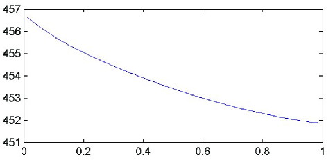
Figure 1: A distribution resulted from the selective pressure. Here is the distribution in a single site shown; there are no beings in other one.

Thus, the approach based on the principles of evolutionary optimality s1 ; s2 ; s3 opposes the diffusion methodology; originally, these principles have been introduced by J.B.S. Haldane. From the point of view of the dynamics of spatially distributed communities, these principles force the individuals to migrate in the manner to increase the net reproduction (NRC). NRC is an average number of descendants (per capita) determined over a sufficiently long generations chain. In brief, a model based on the the principles should look like the following. Consider a population occupying two sites; a transfer from site to site makes a migration. No other movements, inevitable in any real situation, would be taken into account; moreover, we shall suppose that such movements have no impact on the dynamics.

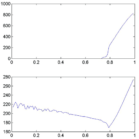
Figure 2: The case of suppressive selection: the beings of the peculiar mobility class ($p=0.8$) are eliminated.

Suppose, then, that the dynamics of each subpopulation follows the Verchulst’s equation:

$$N_{t+1}=N_{t}\cdot\left(a-bN_{t}\right),$$ (1a)

and

$$M_{t+1}=M_{t}\cdot\left(c-dM_{t}\right)\,.$$ (1b)

Here $N_{t}$ ($M_{t}$, respectively) is the subpopulation abundance determined at the time moment $t$. We shall consider the dynamics in discrete time; continuous time consideration is possible, as well, while it bring nothing new, but the severe technical difficulties.

We have chosen the Verchulst’s equation due to its universality s4 . The linear functions in (1) are NRC, in relevant sites. Thus, a migration from one site to another starts up, as soon, as the living conditions (measured as a part of NRC) becomes worse here, in comparison to similar ones there, with respect to the transfer cost $p$, $0\leq p\leq 1$. This latter may be considered as a probability of a successful transfer from a station to another one, with no damage of a further reproduction. Evidently, an additive pattern of a transfer cost is the simplest one:

$$p=p_{\textrm{out}}+p_{\textrm{in}}+d\,,$$

where $p_{\textrm{out}}$ is the cost of a successful leaving of the site; $p_{\textrm{in}}$ is the cost of a successful intrusion into another site, and $d$ is the pure transfer cost.

We shall suppose that the individuals under consideration are globally informed; in such capacity, it means here, that all the parameters (including the transfer cost), as well, as the abundances in each site are known to them.

The N $\mapsto$ M migration takes place, as

$$a-b\cdot N<p\cdot\left(c-d\cdot M\right)\,,$$ (2)

and the reverse migration takes place, when

$$c-d\cdot M<p\cdot\left(a-b\cdot N\right)\,.$$ (3)

The number of migrants must equalize the inequality (2) (or the inequality (3), respectively):

$$a-b\cdot(N-\Delta)=p\cdot\left(c-d\cdot(M+p\cdot\Delta)\right)$$ (4)

or

$$c-d\cdot(M-\Delta)=p\cdot\left(a-b\cdot(N+p\cdot\Delta)\right)\,,$$ (5)

respectively. Since the number of emigrants may not exceed the total abundance observed within a station, then, finally, the migration flux $\Delta$ is determined according to

$$\Delta=\min\left\{N_{t},\ \frac{pc-a+dN_{t}-pdM_{t}}{b+p^{2}d}\right\}\,\,\,\phantom{\textrm{.}}$$ (6a)

or

$$\Delta=\min\left\{M_{t},\ \frac{pa-c+dM_{t}-pbN_{t}}{d+p^{2}b}\right\}\,.$$ (6b)

Here (6a) corresponds to N $\mapsto$ M migration, and vice versa.

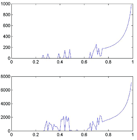
Figure 3: An occurrence of several subspecies differing in mobility. It is clearly evident, that some classes of $p$ are eliminated. Upper figure corresponds to $N$ site, and lower one to $M$ site.

III Modification of the basic model

Suppose, a population (in both sites) is divided into $K$ classes, with respect to the mobility character. This latter is measured as transfer cost peculiar for each class:

$$0\leq p_{1}<p_{2}<\ldots<p_{K-1}<p_{K}\leq 1\,.$$

Let, then, $N_{t}^{(j)}$ ($M_{t}^{(j)}$, respectively) be the abundance of of a subpopulation at $j\textrm{-th}$ class. The dynamics of a subclass (at a subpopulation) is determined according to the equation:

$$N_{t+1}^{(j)}=N_{j}^{(j)}\cdot\left\{a-b\cdot\dfrac{1}{K}\displaystyle\sum_{j=1}^{K}N_{t}^{(j)}\right\}\,{;}$$ (7a)

$$M_{t+1}^{(j)}=M_{t}^{(j)}\cdot\left\{c-d\cdot\dfrac{1}{K}\displaystyle\sum_{j=1}^{K}M_{t}^{(j)}\right\}\,.$$ (7b)

Migration rule keeps the same, as (2) and (3), for each class, with $p_{j}$ peculiar for the class. So, the migration fluxes are determined independently, at each mobility class (i. e., for each $p_{j}$), the beings relocate themselves between the sites, and finally the reproduction takes place.

IV Results and Discussion

We simulated the dynamics of the system (1 – 7), for various parameters. Obviously, the system is symmetric: nothing will change, if one simulate the dynamics originally for $a=\alpha$, $b=\beta$, $c=\gamma$ and $d=\theta$, and then do it for $a=\gamma$, $b=\theta$, $c=\alpha$ and $d=\beta$. This symmetry allows to decrease the dimension of the system. Three parameters control the system: these are $a$, $c$ and $\lambda=b/d$.

We have simulated the dynamics of the system (1 – 7) for $\lambda=1$, $\lambda=1/2$, $\lambda=1/4$ and $\lambda=1/10$. The simulation was run in the manner ro scan the parameters $a$ and $c$ area searching the stable polymodal distribution of the the beings over the transfer cost values. Moreover, in case of $\lambda=1$, there is a symmetry against the permutation of the parameters of $a$ and $c$.

Further, we show several figures illustrating the observed distributions. Fig. 1 shows the

Figure 4: Another example of disruptive selection.

distribution observed at $\lambda=1/4$ and $a=4$, $c=0.1$. The observed distribution is a typical pattern, for the case of so called selective pressure: the abundance of the classes with decreasing mobility grows up monotonously. The figure shows quite rare situation, when the beings with low mobility (small $p$) take an advantage under the selection pressure.

Figure 2 shows an interesting case of the suppressive selection: a peculiar mobility class ($p=0.8$). This kind of the distribution might be considered as a partial case of disruptive selection. Similar situation is shown in Fig. 4; again only one site is shown, since the other one is not inhabited. This figure is obtained for $\lambda=1/2$, and $a=0.1$, $c=8.7$.

Figure 3 shows the situation that is clearly understood as the dissolution of originally homogeneous (and continuously distributed over the mobility factor $p$) population into two discrete subspecies. Some classes are completely eliminated due to the selection. Here only few classes have survived; the survival of the most mobile classes seems rather natural, while the pattern shown in Fig. 1 puts on a hypothesis that there are some parameters vales that would yield the survival of the slower beings, while the faster ones would be eliminated. Finally, Figure 4 shows the situation of the elimination of the peculiar classes, while the majority of them survive.

The paper aims to illustrate the occurrence of the selection based on the mobility of organisms, in case of a non-random migration. Actually, such selection is not a trick: according to the fundamental theorems on the selection, everything that is inherited, must be processed through the selection s1 ; s2 ; s3 ; s4 . This fact explains the results observed at the simulation experiments.

Obviously, one can argue, that there are no species that are present by the beings with all possible diversity of a parameter (the mobility $p$, in our case). That is right; here we just went the way very peculiar for a modelling in biology. We have changed the potential diversity of the beings with mobility $p$ that may appear within a population due to mutation for the actual diversity, as if all the mutations already have been done.

References

- (1) T.K. BenDor, S.S. Metcalf 2006. The spatial dynamics of invasive species spread // Syst. Dyn. Rev. 22, pp.27–50.
- (2) S. Engen 2007. Heterogeneity in dynamic species abundance models: The selective effect of extinction processes // Mathematical Biosciences, 210, pp.490–507.
- (3) M.A. Nowak (2006) Evolutionary dynamics : exploring the equations of life The Belknap Press. 357 p.
- (4) A. Traulsen, M.A. Nowak, J.M. Pacheco 2006. Stochastic dynamics of invasion and fixation // Phys. Rev. E, 74, 011909.
- (5) J.H. Brown 1984. On the relationship between abundance and distribution of species // Am. Nat. 124, pp.255–279.
- (6) T.J. Case, M.L. Taper 2000. Interspecific competition, environmental gradients, gene flow, and the coevolution of species borders // Am. Nat. 155, pp.583–605.
- (7) R. Gomulkiewicz, R.D. Holt, M. Barfield 1999. The effects of density-dependence and immigration on local adaptation in a black-hole sink environment // Theor. Popul. Biol., 55, pp.283–296.
- (8) A.T.C. Silva, J.F. Fontanari 1999. Deterministic group selection model for the evolution of altruism // Eur. Phys. J. B. 7, pp.385–392.
- (9) V. Volterra 1931. Leçons sur la théorie mathématique de la lutte pour la vie. Paris: Gauthier-Villars.
- (10) A.J. Lotka 1922. Natural selection as a physical principle // Proc. Natl. Acad. Sci., 8, pp. 151–54.
- (11) A.N. Gorban 1984. Equilibrium encircling. Nauka plc., Novosibirsk, 226 p.
- (12) A.N. Gorban 2004. Systems with inheritance: dynamics of distributions with conservation of support, natural selection and finite-dimensional asymptotics // arXiv:cond-mat/0405451
- (13) A.N. Gorban 1992. Systems with inheritance and selection effects // in: Evolutionary modelling and kinetics. Novosibirsk: Nauka plc. pp.40–72.
- (14) Ch. Darwin 1897. Origin of species. / Springer-Verlag.
- (15) J.B.S. Haldane, 1931. Selection intensity as a function of mortality rate // Proc. of the Cambridge Philos. Soc. vol. 27. pp. 131–136.
- (16) J.B.S. Haldane, 1934. Some theorems on artificial selection // Genetics. vol. 19. pp. 412–429.
- (17) A.N. Gorban, V.A. Okhonin, M.G. Sadovsky, R.G. Khlebopros 1985. Validity conditions of the simplest equation of mathematical ecology / In: Problems of environmental monitoring and modelling of ecosystems, Leningrad: Gidrometeoizdat, 7, pp.235–241.