Ab initio simulation of photoemission spectroscopy in solids:
Plane-wave pseudopotential approach, with applications to normal-emission spectra of Cu(001) and Cu(111)

Abstract

We introduce a new method for simulating photoemission spectra from bulk crystals in the ultra-violet energy range, within a three-step model. Our method explicitly accounts for transmission and matrix-element effects, as calculated from state-of-the-art plane-wave pseudopotential techniques within density-functional theory. Transmission effects, in particular, are included by extending to the present problem a technique previously employed with success to deal with ballistic conductance in metal nanowires. The spectra calculated for normal emission in Cu(001) and Cu(111) are in fair agreement with previous theoretical results and with experiments, including a newly determined spectrum. The residual discrepancies between our results and the latter are mainly due to the well-known deficiencies of density-functional theory in accounting for correlation effects in quasi-particle spectra. A significant improvement is obtained by the LDA+$U$ method. Further improvements are obtained by including surface-optics corrections, as described by Snell’s law and Fresnel’s equations.

I Introduction

Photoemission spectroscopy (PES) is one of the most basic techniques for investigating the electronic properties of solids. Hüfner (1995); Feuerbacher and Wilis (1976) In practice, however, it is difficult to extract information directly from the observed spectra and theoretical considerations are necessary for a precise determination of the underlying transitions. The modeling of photoemission, as well as the type and accuracy of the information that can be gained from experiments, depends on the energy range of the incident light. In the energy range of ultra-violet photoemission spectroscopy (UPS, between $5$ and $100$ eV), the spectra are dominated by wavevector-conserving transitions (direct transitions) with transition matrix elements differing significantly for any pair of initial and final states. Hence, in UPS, final-state effects play a major role. In empirical approaches these final states are often modeled by free-electron bands, but, in reality, they are influenced by the crystal potential especially at low photon energies and, therefore, their proper description requires detailed calculations.

Early photoemission calculations, ranging from one-electron approaches to many-body formulations, Adawi (1964); Mahan (1970); Schaich and Ashcroft (1971); Caroli et al. (1973); Feibelman and Eastman (1974) covered various aspects of the photoemission process. One-electron photoemission calculations started with the so-called three-step model,Berglund and Spicer (1964) which breaks the photoemission process into three independent steps: excitation of the photoelectron, its transport through the crystal up to the surface, and its escape into the vacuum. Inclusion of quasiparticle lifetimes through adjustable parameters, within the multiple-scattering Green’s function formalism, led to the development of the one-step model.Pendry (1976) Its modern versions can model surfaces by a realistic barrierGraßet al. (1993a) and have the potential of replacing the previously adopted muffin-tin potentials by space-filling potential cells of arbitrary shape,Graßet al. (1993b) also taking into account relativistic effects.Graßet al. (1994)

Ab initio methods based on density functional theory (DFT) are nowadays considerably developed.Martin (2004); Baroni et al. (2001) In particular, the plane-wave (PW) pseudopotential (PP) formulation is being applied to a wide range of properties and systems. Relativistic effects can be included in the PP both at the scalar relativistic or at the fully relativistic level, thus accounting for spin-orbit coupling.Dal Corso and Mosca Conte (2005) This methodology, in principle, contains many of the ingredients necessary to predict a photoemission spectrum from first principles, from which information on various physical properties of the system can then be extracted. In the case of X-ray photoemission, for instance, the observed spectra are routinely compared with the density of electronic states. Considerable complications, however, arise in the ab initio simulation of UPS spectra, as well as in their interpretation, so that the application of state of-the-art DFT PW-PP techniques to this problem has hardly been attempted so far. First and foremost comes the difficulty of accounting for the nonperiodic nature of the electronic states involved in the photoemission process. One of the few attempts to compute photoemission spectra using PPs was made by Stampfl et al.Stampfl et al. (1993) who constructed the final states by a low-energy electron diffraction (LEED) computational technique. Second, and no less important, is the well-known inability of DFT to properly account for self-energy effects on the quasiparticle states that are the main concern of PES. This failure of DFT to accurately describe quasiparticle states is the field of intense research, currently mainly addressed using techniques from many-body perturbation theory, such as, e.g., the GW approximation. Aryasetiawan and Gunnarsson (1998); Marini et al. (2001); Botti et al. (2007)

In this paper the first problem is thoroughly addressed by calculating the transmission of electrons from the crystalline medium into the vacuum by a technique that was previously successfully employed to deal with the ballistic conductance of an open quantum system within the Büttiker-Landauer approach.Choi and Ihm (1999) This technique, originally formulated with norm-conserving PPs, has been generalized to ultrasoft (US) PPs by Smogunov et al.,Smogunov et al. (2004) and this generalization is used here to calculate the transmission into the vacuum of the crystalline Bloch states. In addition to transmission, a completely ab initio approach to PES would require the calculation of dipole matrix elements and a proper account of self-energy effects on the electron band structure, as well as of the effects of the change of the dielectric function upon crossing the surface (surface-optics effects). Dipole matrix elements are calculated completely ab initio using a technique first described by Baroni and Resta in 1986.Baroni and Resta (1986) The real part of the self-energy shifts to DFT bands is accounted for semi-empirically using the LDA+$U$ method, while the imaginary part (lifetime effects) is simply added as an empirical parameter. Finally, surface-optics effects are accounted for by the Snell’s and Fresnel’s equations. While these equations could in principle be implemented using a dielectric function calculated ab initio, for simplicity we choose to implement them using experimental data.Weaver et al. (1981)

As an application of our approach, we calculate the bulk contributions to the normal photoemission spectra from Cu$(001)$ and Cu(111). Copper is a prototypical system for UPS studies, for which many theoretical results, as well as accurate experimental measurements, are available. We compare our calculations with previous theoretical studies, performed within the one-step and three-step models, and with experimental data. Not surprisingly, the main limiting factor in our calculations appears to be the poor description of the Cu electron bands by the local-density approximation (LDA), while transmission effects are correctly accounted for, thus providing a viable way to select and to weigh among the many available final conduction states only those that couple to vacuum states.

The paper is organized as follows: in Sec. II we describe the theoretical method used to calculate photoemission spectra, while in Sec. III we give some numerical details. In Sec. IV we first discuss the contributions of different terms in our expression for the photoemission intensity, on one specific example; we then present our ab initio results for the Cu(001) surface, obtained at the DFT level without empirical adjustments, followed by the results for Cu(001) and Cu(111) obtained from LDA+$U$ bands and accounting for surface-optics effects. Sec. V contains our conclusions.

II Theory

In a three-step model, the photoemission current is proportional to the product of the probability that an electron is excited from an initial bulk state, $\psi_{i}$, to an intermediate bulk state, $\psi_{n}$, of energies $E_{i}$ and $E_{n}$ and wavevector $\mathbf{k}$, $|M_{ni}(\mathbf{k})|^{2}$ (in this transition the electron momentum is supposed to be conserved, in spite of surface effects that break translational symmetry), times the probability that the electron in the intermediate state is transmitted into the vacuum, $T(E_{n},\mathbf{k})$, conserving the energy and the component of the momentum parallel to the surface, $\mathbf{k}_{\parallel}$. Summing the composite probabilities all over the possible initial and intermediate states, we obtain the current, $I$, as a function of the photo-electron kinetic energy, $E_{\rm kin}$, and photon energy, $\hbar\omega$, using the standard expression:D.Grobman et al. (1975); Smith et al. (1980); Hüfner (1995)

$$I(E_{\rm kin},\hbar\omega,{\bf k_{\parallel}})\propto\sum_{ni}\int dk_{\perp}|M_{ni}({\bf k})|^{2}T(E_{n},{\bf k})\delta[E_{n}({\bf k})-E_{i}({\bf k})-\hbar\omega]\delta[E_{\rm kin}-E_{n}({\bf k})+\Phi],$$ (1)

where $k_{\perp}$ is the component of $\mathbf{k}$ perpendicular to the surface and $\Phi$ the work function. The three-step model that we use is, of course, an approximation which, in particular, does not properly account for coherence between the excitation process occuring in the bulk and the escape of the electron, occuring at the surface. This coherence may give rise to interference effects which are, therefore, neglected in our approach.

The transition matrix element in Eq. (1), $M_{ni}$, is calculated from the interaction operator:

$$H_{\rm int}=\frac{e}{2mc}({\bf A\cdot p}+{\bf p\cdot A}),$$ (2)

where A is the vector potential of the electromagnetic field and p the momentum operator of the electron, $e$ and $m$ are the electron charge and mass, $c$ is the speed of light, and nonlinear effects have been neglected. We will consider only the ${\bf A\cdot p}$-type interaction, while the $\nabla A$-interaction, originating from the second term in Eq. 2 and giving rise to surface emission (the gradient of A is significant only in a very narrow region around the surface), is neglected, in accord with common practice in photoemission calculations.Pendry (1976) In this paper, we shall consider normal photoemission only, i.e. ${\bf k_{\parallel}}=0$. Energy conservation is imposed by the two $\delta$-functions. In the dipole approximation, A can be considered spatially constant (the wavelength of the photon beam, which is 120-2500 Å  in the UPS energy range, is very large compared to the atomic spacing in crystal) and therefore the transition matrix elements are proportional to the dipole matrix element between the propagating initial and intermediate states:

$$M_{ni}=\frac{e}{mc}{\bf A}\langle\psi_{n}|{\bf p}|\psi_{i}\rangle.$$ (3)

The vector potential A carries information on the light polarization, depending on the polar ($\theta$, defined with respect to the surface normal) and azimuthal ($\phi$) angles of incidence of the photon beam. In this paper, we consider linearly polarized electromagnetic radiation, with the following convention: for $p$-polarized light, A is contained within the plane formed by the directions of the incident light and outgoing electron, while for $s$-polarized light, A is perpendicular to this plane. Thus, for $s$-polarized light $\mathbf{A}$ is parallel to the surface for normal photoemission.

In general, when an electromagnetic plane wave impinges on a metal surface, the value of the vector potential transmitted inside the metal differs from the value in the vacuum, due to the departure from unity of the medium dielectric function, $\epsilon(\omega)$.Weaver et al. (1981) The transmitted vector potential ${\bf A}^{t}$ can be calculated from the incident field ${\bf A}^{i}$, as described by Fresnel’s equations, derived by using the Maxwell’s theory and Snell’s lawBorn and Wolf (1970). Actually, the difference between ${\bf A}^{t}$ and ${\bf A}^{i}$ can be very large, especially for small photon energies ($\hbar\omega<20$ eV) and large $\theta$, as extensively discussed in literature.Feibelman (1974); Whitaker (1978); Smith et al. (1980); Goldmann et al. (1983); Wern and Courths (1984, 1985)

In order to calculate the transmission factor, T($E_{n},{\bf k}$), we take into account that the final state of the photoemission process is a time-reversed LEED (TRL) state, which, sufficiently far from the surface is free-electron-like in the vacuum (outer region), while inside the crystal (inner region) it is a linear combination of the Bloch states available at the intermediate energy, $E_{n}$. The TRL state can thus be obtained by solving the one-electron Kohn-Sham (KS) Schrödinger equation, subject to the appropriate boundary condition in the outer region. This task is accomplished by matching the wavefunctions in the inner and outer regions, using a method proposed by Choi and Ihm,Choi and Ihm (1999) originally devised to cope with ballistic conductance and later generalized to account for US PP’s.Smogunov et al. (2004) In the outer region the TRL state is a plane wave whose wavevector has a component perpendicular to the surface equal to $k_{\perp}=\sqrt{2mE_{\rm kin}/\hbar^{2}-{\bf k}_{\parallel}^{2}}$. For given values of the photoelectron kinetic energy, $E_{\mathrm{kin}}$, and parallel momentum, $\mathbf{k}_{\parallel}$, in the inner region the TRL state reads:

$$\phi^{TRL}_{E_{\mathrm{kin}},{\bf k}_{\parallel}}({\bf r})=\sum_{m}\psi_{n}({\bf r},{\bf k}_{m\perp})t(E_{n},{\bf k}_{\parallel},{\bf k}_{m\perp}),$$ (4)

where the sum is over all the Bloch states available at the intermediate energy $E_{n}=E_{\mathrm{kin}}+\Phi$. In the intermediate region, the TRL depends on the details of the self-consistent potential at the surface, and this dependence determines the relative amplitude of the wavefunctions in the outer and inner regions, hence the transmission coefficient. In practice, the solution of the KS Schrödinger equation by the method of Choi and IhmChoi and Ihm (1999) provides the coefficients of the expansion of the final photoemission state in Bloch waves. These coefficients, which usually yield the total transmission and hence the ballistic conductance, can be used to calculate the transmission probability into vacuum $T(E_{n},{\bf k})=|t(E_{n},{\bf k})|^{2}$ separately for each conduction band. We note that in this approach the scattering state is normalized in such a way that both the incident plane wave and the Bloch states carry unit current.

We now discuss the way in which the two delta functions appearing in Eq. 1 can be treated in practice. The first delta function imposes energy conservation in the excitation step of the photoemission process, while the second one relates the kinetic energy measured outside the crystal to the intermediate state energy, accounting for the work function. The first delta function is usually represented as a Lorentzian:

$$\delta[E_{n}({\bf k})-E_{i}({\bf k})-\hbar\omega]=\frac{\Gamma_{h}/2\pi}{[E_{n}({\bf k})-E_{i}({\bf k})-\hbar\omega]^{2}+\Gamma_{h}^{2}},$$ (5)

which corresponds to the spectral function of the hole left behind by the excitation processMatzdorf (1998) and results in the broadening of the initial state. The width of the distribution, $\Gamma_{h}$, gives the inverse lifetime of the hole, and is equal to the absolute value of the imaginary part of the hole self-energy. As in the majority of other photoemission studies, we take $\Gamma_{h}$ as an adjustable parameter. The second delta function should be replaced by the analyzer resolution function, most commonly expressed in the form of a Gaussian:

$$\delta[E_{\rm kin}-E_{n}({\bf k})+\Phi]=\frac{1}{\sqrt{2\pi}\Gamma_{det}}\exp\Big{[}-\frac{1}{2}\frac{[E_{\rm kin}-E_{n}({\bf k})+\Phi]^{2}}{\Gamma_{det}^{2}}\Big{]}.$$ (6)

$\Gamma_{det}$ is determined by the detector resolution, and is related to the experimental energy broadening.Matzdorf (1998)

We conclude by noticing that the bulk-emission model of photoemission neglects electron damping caused by the presence of a surface. It is implicitly assumed in Eq. 1 that ${k_{\perp}}-$conservation is perfect and the delta function for this conservation law is omitted. The ${k_{\perp}}-$conservation, $\delta({k}_{n\perp}-{k}_{i\perp}-{G_{\perp}})$, is usually represented by a Lorentzian, whose broadening parameter describes damping.Matzdorf (1998) The consideration of only bulk-emission is a good approximation if the damping is small, i.e. if its inverse, the electron escape length, $l_{e}$, is long enough, at least a few lattice spacings. The escape length can be estimated from the relation: $1/l_{e}=\Gamma_{n}\cdot\delta k_{\perp}/\delta E_{n}$,Courths et al. (1979) where $\Gamma_{n}$ stands for the inverse lifetime of the intermediate state and $\delta k_{\perp}/\delta E_{n}$ is the inverse group velocity of the intermediate state. The escape length depends on the band structure through $\delta k_{\perp}/\delta E_{n}$ term and on the photon energy through the empirical dependence of $\Gamma_{n}$ on the intermediate-state energy. Empirically one can use the relationship: $\Gamma_{n}=0.065\cdot E_{n}$.Matzdorf (1998)

III Numerical details

All the ingredients necessary to apply the theory outlined in Sec. II are calculated using DFT within the PW-PP approach, as implemented in the PWscf code of the Quantum ESPRESSO distribution.Baroni et al. In particular, the calculation of transmission coefficients has been performed from the output of the PWcond component contained therein. For the exchange and correlation energy, we use the local density approximation (LDA) with the Perdew-Zunger parametrization.Perdew and Zunger (1981) The interaction of the valence electrons with the nuclei and core electrons is described by a Vanderbilt US PP.Vanderbilt (1990) The use of the PP method for simulating PES deserves some comments and requires care. Modern PPs are usually designed to reproduce very faithfully the electronic structure (orbital energies and one-electron wavefunctions outside the atomic core region) of occupied states. Standard arguments based on the transferability concept ensure that the quality of the electronic structure predicted by PPs is as good in the energy range immediately above the Fermi energy ($E_{F}$), i.e. in an energy range that extends up to, say, 10-15 eV above $E_{F}$. In the present case, however, a particular care has to be taken in describing the intermediate state of the transitions, because these lie at a higher energy than the transferability range of currently available PPs. For this reason, we have decided to generate a highly accurate US PP, specially designed for the purposes of the present work. We used the $3d^{10}4s^{1}4p^{0}$ atomic configuration of Cu, with the core radii: $r_{s}=2.1$, $r_{p}=2.4$, $r_{d}=2.0$ a.u. and two projectors in each of the $s$, $p$, and $d$-channels, one of which was chosen correspondingly to an atomic state chosen at higher energy than usually done.PP_ The PP energy bands thus obtained agree within 0.05 to 0.20 eV with those calculated from a highly accurate all-electron method, using the WIEN2k code,Blaha et al. (2001) up to 40 eV above $E_{F}$. Ordinary Cu PPs, generated without high-energy projectors, tend to miss some unoccupied electron bands and have larger deviations from the all-electron results with increasing energy.

To calculate T($E_{n},{\bf k})$, we used the self consistent potential of a nine-layer tetragonal slab along the [001] direction separated by a vacuum space equivalent to eleven layers. We chose a vacuum space with length equal to two bulk layers as the unit cell in the left lead and two central bulk-like layers of the slab as the periodic unit cell of the right lead. We used the experimental lattice constant ($a=3.62~{}\mathrm{\AA}$) without relaxing the surface layers. However, our calculation allowing relaxations along the perpendicular direction predicts $-2.8$ % relaxation for the first layer, $0.6$ % for the second, and $0.2$ % for the third. We checked that transmission factors change only negligibly with surface relaxations in this case. Kinetic energy cutoffs of $45$ Ry and $450$ Ry have been used for the expansion of the wave functions and of the charge density, respectively. These cutoffs, which are unusually large for US PPs, are a consequence of the improved transferability that we required from our custom-tailored PP. A Monkhorst-Pack meshMonkhorst and Pack (1976) $18\times 18\times 1$ was used for the slab calculation. The band structure and the matrix elements of the dipole operator were calculated from a bulk calculation in which $k_{\perp}$ was sampled by 860 k-points. The matrix elements of the dipole operator have been compared to the matrix elements from the WIEN2K code, finding an agreement of the order of 4% for the states of interest in this paper. For the evaluation of the second delta-function from Eq. 6 we calculated the work function as the difference between the Fermi level and the electrostatic potential in the vacuum, and found $\Phi=4.84$ eV, which is in agreement with previous calculationsFavot et al. (2001) and very close to the experimental values ranging from $4.59$ to $4.83$ eV.wor (a) For Cu(111), our LDA calculations gave the value of 5.08 eV, in good agreement with a previous calculation (5.10 eV)Polatoglou et al. (1993) and experiment (4.9 and 4.94 eV)wor (b) The broadening parameters which appear in Eq. 5 and 6 are chosen as $\Gamma_{h}=0.04$ eV and $\Gamma_{det}=0.07$ eV.

IV Results

In this section we first illustrate our method by discussing the various contributions to the spectrum, as calculated from Eq. (1), for Cu(001) at one specific photon frequency ($\hbar\omega=23$ eV) and for one specific angle of incidence ($\theta=65^{o}$) of the incoming photon beam of $p$ polarization. We then present calculations for a more extensive set of frequencies and incidence angles. Finally, we try to correct the two main sources of errors in our calculations by studying how the spectra are modified by the LDA+$U$ bands and by surface optics. The corrected spectra are presented also in the case of Cu(111) surface.

IV.1 Illustration of the method

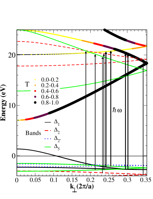
Figure 1: (Color online) Band structure of bulk Cu along the $k_{\perp}$ direction for the Cu(001) surface. We indicated, among the unoccupied bands, those that have a transmission probability into vacuum larger than 0. Different point size and colors indicate different transmission probability. The zero of the energy is at the Fermi level. The direct transitions for $\hbar\omega=23$ eV are presented by arrows, while the four direct transitions which are simultaneously allowed and have non-zero transmission and dipole matrix element are shown with thick arrows.

In Fig. 1 we show our calculated energy bands of bulk Cu. The bands are plotted in the $\Gamma-Z$ direction, along [001]. These correspond to the bands along the $\Gamma-X$ direction in the fcc Brillouin zone (BZ) refolded in the tetragonal BZ. On top of the empty bands in Fig. 1, we add information regarding $T(E_{n},\mathbf{k})$, wherever it is greater than 0. This is possible because $T(E_{n},\mathbf{k})$ explicitly depends on $k_{\perp}$ on the intermediate states.not Thus, reading from Fig. 1 at each intermediate energy, we can find if the propagating final states exist ($T>0$), and if so, for which values of the intermediate $k_{\perp}$. In agreement with empirical intermediate-state determinations, Courths and Hüfner (1984) we find that a free-electron-like band properly modified by the ionic PP has the strongest coupling to the vacuum state. All the bands with nonvanishing transmission probability belong to the $\Delta_{1}$ representation. This is a result of the selection rules for normal photoemission, which impose that the intermediate state be totally symmetric with respect to all the $C_{4v}$ symmetry operations. Combining this result with the symmetry properties of the dipole matrix element we obtain the allowed transitions for normal photoemission from the (001) surface of an fcc crystal: for the $z$-polarization only $\Delta_{1}\rightarrow\Delta_{1}$ transition is allowed, while for the $x$/$y$-polarization $\Delta_{5}\rightarrow\Delta_{1}$ transitions are allowed. Hermanson (1977); Hüfner (1995) Note, however, that some bands with $\Delta_{1}$ symmetry might not be transmitted into vacuum, so symmetry alone would not be sufficient to identify the intermediate states. In the same figure, we also display nine direct transitions present in the case $\hbar\omega=23$ eV. Out of these transitions, only four satisfy selection rules and have dipole matrix elements and transmission factors which are both non-zero. Two of these transitions are of the $\Delta_{1}\rightarrow\Delta_{1}$ type and remaining two of the $\Delta_{5}\rightarrow\Delta_{1}$ type. Only one transition ($\Delta_{1}\rightarrow\Delta_{1}$) has large transmission factor and large dipole matrix element, while the other of the same type has small transmission factor. Both transitions of the $\Delta_{5}\rightarrow\Delta_{1}$ type have small dipole matrix element and one of them even a small transmission factor (smaller than 0.2).

In Fig. 2 we illustrate the influence of the dipole matrix elements and of the transmission factors on the shape of the spectrum. In panel a we show all the direct transitions, regardless of the symmetry, their dipole matrix elements, and the transmission coefficients. In panel b we calculate the photoemission spectrum setting the transmission factor to one for all the bands. We find that the peaks with non-zero dipole matrix elements correspond to $\Delta_{2}\rightarrow\Delta_{2}$ and $\Delta_{1}\rightarrow\Delta_{1}$ ($\Delta_{2}\rightarrow\Delta_{5}$, $\Delta_{5}\rightarrow\Delta_{5}$, $\Delta_{5}\rightarrow\Delta_{2}$, $\Delta_{2^{\prime}}\rightarrow\Delta_{5}$ and $\Delta_{5}\rightarrow\Delta_{1}$) transitions for $z$-polarization ($x$/$y$-polarization), although the transitions with $\Delta_{5}$ and $\Delta_{2}$ intermediate states are not allowed for the normal emission. Including the dipole matrix elements, we obtain a spectrum in which the intensity of the peaks may change. The polarization and the direction of the incident photon beam now play an important role. For $\theta=65^{\circ}$ the $z$-polarized transitions are enhanced with respect to transitions due to $x$/$y$-polarized light. However, neglecting the probability of the intermediate states to be transmitted to vacuum we still have many transitions into $\Delta_{2}$ and $\Delta_{5}$ intermediate states which have finite intensity. Also, the relative intensities of peaks with $\Delta_{1}$ intermediate states are incorrect. The introduction of the transmission factor not only selects the intermediate states with $\Delta_{1}$ symmetry, but also modulates the peak intensities. Thus, two peaks shown in panel c) originate from the $\Delta_{1}$ initial state, while the shoulder of the main peak on the high-energy side and almost invisible shoulder to the high-energy peak originate from the $\Delta_{5}$ initial state. We note that, at variance with the rest of the paper, in Fig. 2 we used smaller broadening parameters $\Gamma_{h}=\Gamma_{det}=0.015$ eV, in order to separate the different peaks.

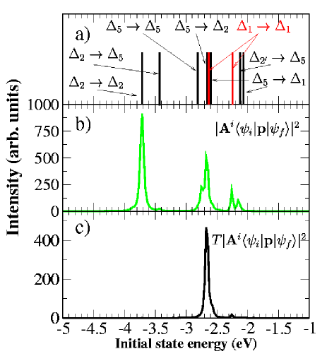
Figure 2: (Color online) Influence of dipole matrix elements and transmission factors on the spectrum for $\hbar\omega=23$ eV and $\theta=65^{\circ}$. Panel a) presents all the allowed transitions with an indication of the symmetry of the initial and intermediate states. Panel b) shows the effect of the dipole matrix elements. Panel c) shows the effects of the transmission factors.

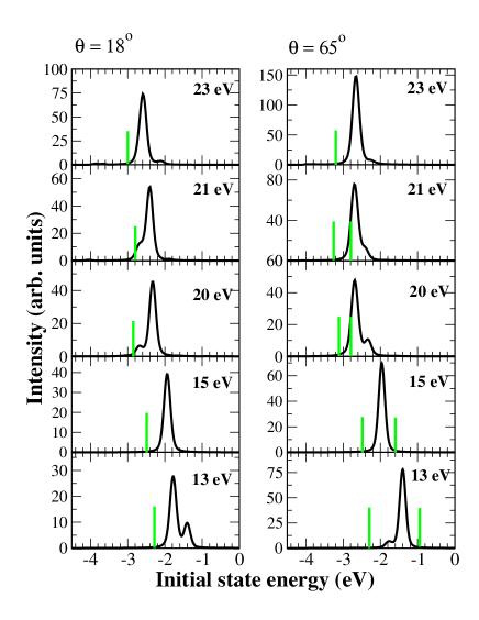
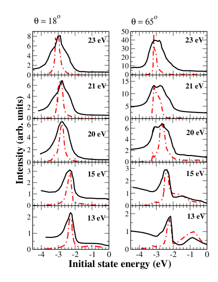
Figure 3: (Color online) Calculated photoemission intensity for Cu(001) (left panels). The experimental spectra (dashed line), together with a previous calculation (darker full line)Baalman et al. (1986) are shown on the right. The spectra in both panels are given for various photon frequencies and for two incident angles, $\theta=18^{\circ}$ (on the left of each panel) and $\theta=65^{\circ}$ (on the right). The sticks in the left panels indicate positions of the main experimental peaks.

IV.2 Ab initio results

In the left panel of Fig. 3 we present our calculated spectra for five photon frequencies between $13$ and $23$ eV and two incident angles $\theta=18^{\circ}$ and $\theta=65^{\circ}$ for the $p$-polarization. In the right panel, we show for comparison the experimental and previous theoretical normal-emission spectra for the same frequencies and angles.Baalman et al. (1986) Previous calculations were performed within the one-step model,Pendry (1976) based on the non-relativistic empirical muffin-tin potential and taking into account the surface optics through the application of Snell’s law and Fresnel’s equations. Our spectra in Fig. 3 do not include surface-optics effects and are calculated within the bulk photoemission model. The first approximation is quite severe and its effects will be discussed below, while the second should be sufficiently justified for this surface. Actually, for the photon energies considered here, $\delta k_{\perp}/\delta E_{n}$ is smaller than $0.05$ $\mathrm{\AA}^{-1}\mathrm{eV}^{-1}$ and the damping (for an average photon energy of $18$ eV) can be estimated to be less than 0.06 $\mathrm{\AA}^{-1}$. This rough estimate yields the electron escape length of about $10$ lattice spacings in the direction perpendicular to the surface. The choice of the incidence angle influences the spectra significantly: for $\theta=18^{\circ}$, light is mostly polarized in the $xy$ plane, (the initial state belongs to the $\Delta_{5}$ representation), while for $\theta=65^{\circ}$, most emission is from $\Delta_{1}$-like states ($z$-polarization). Overall, our calculation reproduces the majority of the experimental peaks, albeit with a shift of about $0.2$-$0.6$ eV towards higher energies and somewhat altered relative intensities. It is well known that the LDA, as well as generalized gradient approximation (GGA), fails to describe accurately quasi-particle energy bands as measured by PES and, therefore, the incorrect position of the peaks has to be attributed to the error in the calculated bands.Strocov et al. (1998) The calculation within the one-step modelBaalman et al. (1986) is performed with an empirical potential and, therefore, the energy bands correspond to the experimental bands rather well. The error in the positions of energy bands can result also in a reduction or an increase of the number of peaks. At $\theta=18^{\circ}$ and $\hbar\omega=13$ eV the theoretical spectrum shows two peaks, one at $-1.76$ eV and one at $-1.38$ eV. The former is due to a transition from the $\Delta_{5}$ band, while the latter originates from the $\Delta_{1}$ band. Experimentally, only a single peak is present at about $-2.30$ eV. The spectrum for $\hbar\omega=15$ eV shows a single peak as the experiment although at higher energy. The spectra at $\hbar\omega=20,21$ and $23$ eV show only one main peak and a small peak, missing some of the shoulders present in the experimental spectra, a feature that our result has in common with the previous calculation. The lower-energy features in the spectra $\hbar\omega=20$ and 21 eV originate from the $\Delta_{1}$ bands and the higher-energy features from the $\Delta_{5}$ bands. In the spectrum $\hbar\omega=23$, both peaks are predominantly from the $\Delta_{5}$ initial state, although there are significant contributions on the low-energy sides originating from the $\Delta_{1}$ initial states. These contributions are hard to discern due to a large broadening and closeness of the peaks ($\sim 0.1$ eV).

For $\theta=65^{\circ}$ the agreement is somewhat worse. The spectrum for $\hbar\omega=13$ eV has a barely visible feature in place of the main peak of the experimental spectrum while the $\Delta_{1}$ peak is significantly overestimated and at too low energy. As we show below, this will be corrected in part by considering the surface optics. That type of correction is quite large for small photon energies and large incidence angles.Smith et al. (1980) Similarly to the case $\theta=18^{\circ}$, the spectrum for $\hbar\omega=15$ eV has only one peak, which actually contains two transitions (from the $\Delta_{1}$ and $\Delta_{5}$ initial states). Due to our imprecise energy bands, both transitions are accidentally at the same energy. The experimental spectrum for $\hbar\omega=20$ eV has two peaks of roughly equal intensity, with a broad shoulder on the high-energy side, while our spectrum reproduces just one main peak and a much lower-intensity peak at higher energy. Our spectra for $\hbar\omega=21$ and $23$ eV are underestimating or missing a high-energy feature, present in the experimental spectra. We note that in contrast to the $\theta=18^{\circ}$ case, both peaks in the spectrum for $\hbar\omega=23$ eV originate from the $\Delta_{1}$ initial states, and transitions from the $\Delta_{5}$ give small contributions on the high-energy sides, as seen in Fig. 2. Finally, we note that the peak intensities can be compared only within one spectrum, i.e. the intensities for different $\hbar\omega$ cannot be compared in our calculation, due to the neglect of electron damping, which is energy dependent. Consequently, it is clear that the standard ab initio approach needs further corrections to reproduce the fine details of the experimental spectra.

IV.3 Empirical corrections

In this section we try to correct empirically two of the main shortcomings of our approach using quite simple models. It is known that inclusion of self-energy effects, at least within the GW model, would be mandatory for a realistic description of the band structure.Marini et al. (2001) Presently, however, this is beyond our capabilities mainly because it would require a nontrivial extension of the ballistic conductance code. Hence, we choose a simpler approach, using LDA+$U$.Anisimov et al. (1997); Cococcioni and de Gironcoli (2005) LDA+$U$ goes beyond LDA by treating exchange and correlation differently for a chosen set of states, in this case, the copper $3d$ orbitals. The selected orbitals are treated with an orbital dependent potential with associated effective on-site Coulomb interaction $U_{\rm eff}$, which is a function of Coulomb and exchange interactions $U$ and $J$, $U_{\rm eff}=U-J$. Sawada et al. (1997); Dudarev et al. (1998) The LDA$+U$ method is most commonly known as a cure for the inability of traditional DFT implementations to predict the insulating state of some strongly correlated materials.Anisimov et al. (1997) Although the theoretical foundation of LDA$+U$ is somewhat questionable, its range of applicability is wider, and this method has indeed been succesfully applied to metallic systems where the effects of electron correlations are intermediate.Mohn et al. (2001); Stojić et al. (2006); Stojić and Binggeli (2008) LDA$+U$ is also being succesfully employed as a predictive tool in the chemistry of transition-metal molecules.Kulik et al. (2006) Furthermore, in the specific case of bulk copper, there is evidence that an account of self-interaction effects in LDA through the LDA+SIC approach leads to an improvement of the calculated bands.Norman (1984) However, the LDA+SIC approach neglects screening effects on the self-interactions, which are instead accounted for to different degrees of accuracy in the GW and in the LDA+$U$ methods. While GW addresses screening in a more rigorous way, LDA+$U$ can be considered as the static limit of a kind of (admittedly, rather crude) approximation to the GW method.Anisimov et al. (1997)

		LDA	GW	LDA+$U_{1}$	LDA+$U_{2}$	LDA+$U_{3}$	Experiment
Positions of	$\Gamma_{1,2}$	$-2.18$	$-2.81$	$-2.60$	$-2.75$	$-2.92$	$-2.78$
$d$ bands	$X_{5}$	$-1.44$	$-2.04$	$-1.85$	$-2.00$	$-2.17$	$-2.01$
	$L_{3}$	$-1.60$	$-2.24$	$-2.00$	$-2.17$	$-2.31$	$-2.25$
	$\Gamma_{1,2}-\Gamma_{2,5}$	$0.83$	$0.60$	$0.83$	$0.83$	$0.83$	$0.81$
Widths of	$X_{5}-X_{3}$	$2.94$	$2.49$	$3.01$	$3.04$	$3.05$	$2.79$
$d$ bands	$X_{5}-X_{1}$	$3.40$	$2.90$	$3.53$	$3.57$	$3.61$	$3.17$
	$L_{3}-L_{3}$	$1.44$	$1.26$	$1.47$	$1.48$	$1.49$	$1.37$
	$L_{3}-L_{1}$	$3.46$	$2.83$	$3.55$	$3.56$	$3.60$	$2.91$
Positions of	$\Gamma_{1}$	$-9.37$	$-9.24$	$-9.25$	$-9.22$	$-9.19$	$-8.60$
$s/p$ bands	$L_{2}^{\prime}$	$-1.00$	$-0.57$	$-0.88$	$-0.85$	$-0.83$	$-0.85$
$L$ gap	$L_{1}-L_{2}^{\prime}$	$4.04$	$4.76$	$4.67$	$4.88$	$5.10$	$4.95$

Table 1: Comparison of different theoretical (LDA, LDA+GW corrections,Marini et al. (2001) LDA+$U$, $U_{1}=1.5$ eV, $U_{2}=2$ eV and $U_{3}=2.5$ eV) band energies and bandwidths for copper, at high-symmetry points, compared to the average over several experiments (as reported in Tables I and XIII in Ref. Courths and Hüfner, 1984). All values are in eV.

As Cu has an almost completely filled $d$-shell, the main effect of the LDA+$U$ is the shift of the electron bands, while the eigenfunctions are expected to remain quite close to the LDA ones.Anisimov et al. (1997) Actually, we checked that, for the values of $U$ used here, the overlap between the LDA and the LDA+$U$ wavefunctions is of the order of 0.99. Thus, we kept the same transmission and dipole matrix elements calculated with the LDA wavefunctions correcting only the band structure.

Table 1 presents some results, such as the positions of $d$-bands and bandwidths, evaluated using different methods including DFT with LDA, self-energy corrections within GW approximationMarini et al. (2001) calculated on top of ab initio DFT results, LDA+$U$ for three values of $U_{\rm eff}$, all compared to the average over several experimental values.Courths and Hüfner (1984) The positions of the $d$-bands at the $\Gamma$ point vary greatly for different methods. The LDA calculation finds the band $0.6$ eV too shallow, while GW reproduces the experimental value quite well. LDA+$U$ significantly improves with respect to the LDA value and for $U_{\rm eff}=2$ eV gives almost the experimental value. Similar level of precision can be seen for the positions of the $d$-bands at the $L$ and $X$ points, with somewhat larger deviations of the LDA and the LDA+$U$ from the experimental value at the $L$ point. Again, among the three values of $U_{\rm eff}$, at the $L$ and $X$ points the best agreement with experiment is obtained for $U_{\rm eff}=2$ eV. The width of the $d$-band at the $\Gamma$ point is, instead, quite faithfully reproduced both by the LDA and the LDA+$U$. For other special points given in Table 1, the widths remain almost constant for different $U_{\rm eff}$. We note that also the positions of $s/p$-bands and $L$-gap improve with the LDA+$U$. Overall, we conclude that the LDA+$U$ can correct the LDA bands in a significant manner, and has effects comparable to the full self-energy calculation. Also, on the basis of comparison with the experimental results, we find that $U_{\rm eff}=2$ eV gives the best results and we choose to use this value in the rest of the paper.

The second main problem in the calculation of the intensities of the photoemission peaks comes from the fact that the vector potential inside the solid is different from the vector potential in the vacuum. Consequently, one should correct the intensities using the Snell’s law and Fresnel’s equations.Feibelman (1974); Whitaker (1978); Smith et al. (1980); Goldmann et al. (1983); Wern and Courths (1984, 1985) An accurate account of this effect is quite difficult. First of all, one should use a dielectric function calculated consistently within the same ab initio scheme used for the calculation of the other quantities. Furthermore, the effect of the surface should be properly taken into account in the evaluation of the dielectric function. However, as this would require a substantial effort, we choose just to estimate the effect by using the experimental dielectric function from Ref. Weaver et al., 1981.

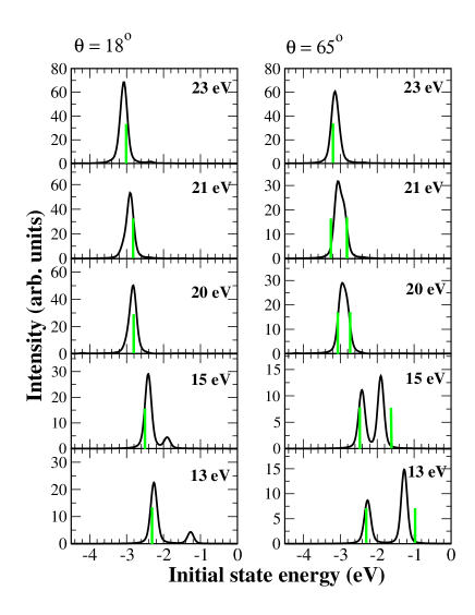
Figure 4: (Color online) Calculated photoemission intensity for various photon frequencies for two incident angles, $\theta=18^{\circ}$ and $\theta=65^{\circ}$ using LDA+$U$ approach, with $U_{\rm eff}=2$ eV. The sticks indicate the positions of the main peaks in the experimental spectra (and previous calculations spectra).

We report in Figure 4 the photoemission spectrum calculated with the LDA+$U$ bands with $U_{\rm eff}=2$ eV and including the surface optics corrections, for the same parameters as in Fig. 3. We checked that the spectra do not show strong dependence on the choice of $U_{\rm eff}$, e.g. for $U_{\rm eff}=1.5$ eV, the spectra are almost identical to the $U_{\rm eff}=2$ eV case, with a small shift in energy.

In comparison with the experimental spectrum from Fig. 3, we see that the energy positions are mostly corrected. For $\theta=18^{\circ}$, the spectrum for $\hbar\omega=13$ eV is improved with respect to the LDA spectrum (Fig. 3), also in terms of the distance and relative intensities of the two peaks. For $\hbar\omega=15$ eV, the two transitions which were at the same initial energy split, giving rise to a new peak. Thus, the lower-energy peak originates from the $\Delta_{5}$ band and the higher-energy one from the $\Delta_{1}$ band. In the one-step calculation there is only a hint of a shoulder on the high-energy side. For $\hbar\omega=20$ and $21$ eV we lose the shoulders originating from the $\Delta_{1}$ initial state, present in the LDA spectra. This is because the bands are shifted in such a way that the transitions happen for ${k_{\perp}}$ at which the two bands are very close in energy, less than 0.2 eV difference. The spectrum for $\hbar\omega=23$ eV looses a higher-energy peak originating from the $\Delta_{1}$ band, as this peak comes under the main peak from the $\Delta_{5}$ band.

For $\theta=65^{\circ}$ all the spectra have significantly lower intensity with respect to the LDA, as a direct consequence of surface-optics corrections. In the spectrum for $\hbar\omega=13$ eV, the positions of the peaks are improved and also the peak intensity ratio goes in the right direction, as a result of the inclusion of $\epsilon(\omega)$. Nevertheless, this correction does not suffice and the intensities of the two peaks remain wrong, both with respect to experiment and with respect to the one-step model. Inspecting the Cu$(001)$ band structure in Fig. 1 we see that for $\hbar\omega=13$ eV the two initial bands actually have different dispersions at the ${k_{\perp}}$ at which transitions are taking place (0.17 and 0.18 $2\pi/a$), whereas the dispersion of the intermediate band (the lowest unoccupied band) does not change significantly between the two ${k_{\perp}}$. The low-energy peak, which is underestimated, originates from the initial band of $\Delta_{5}$ symmetry and has smaller slope at the ${k_{\perp}}$ of the direct transition. Allowing nondirect transitions, due to electron damping, this peak would get many more contributions than the peak originating from a $\Delta_{1}$ band with strong dispersion and would, thus, improve agreement with the experimental spectrum. A similar argument holds also for the spectrum for $\hbar\omega=15$ eV which gets a new peak with respect to the LDA spectrum, but whose intensity is overestimated. For $\hbar\omega=20$ and 21 eV the high-energy peaks (of $\Delta_{5}$ origin) from the LDA spectra are smeared into shoulders, due to the shift of bands. For the same reason, a high-energy shoulder from the LDA spectrum for $\hbar\omega=23$ eV is lost. Overall, we conclude that the LDA+$U$ correction is affecting all the spectra, causing the shift of all peaks, which also results in a decrease or increase of the number of peaks. The surface-optics corrections improve agreement for low photon energies and have stronger effects for $\theta=65^{\circ}$. In general, both corrections improve the agreement with experiment.

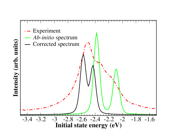
Figure 5: (Color online) Comparison of our Cu(001) ab initio (light-colored full line) and corrected (dark full line) spectra, with the experimental spectrum (dashed line) for $\hbar\omega=17$ eV and $\theta=45^{\circ}$.

Figure 5 compares our ab initio and corrected spectra, with a recently measured experimental spectrum on the Cu(001) surface for $p-$polarization, $\hbar\omega=17$ eV and $\theta=45^{\circ}$. The experimental spectrum was measured on the Cu(001) single crystal surface at APE beamline (TASC, Italy) at room temperature. It was integrated over an angular window of $1^{\circ}$ around the normal emission. The energy resolution was estimated to be 25 meV. Both theoretical spectra have two peaks, the low-energy one originates from the $\Delta_{1}$ initial band and the high-energy one from the $\Delta_{5}$ initial band. The ab initio spectrum has wrong energy positions ($\sim 0.15$ eV too high), the distance between the two peaks is too large and the peak ratio is overestimated ($1.78$ instead of $1.40$). The corrected spectrum shows a better agreement with experiment. The positions of the peaks are closer to the experiment ($\sim 0.07$ eV too deep), the distance between peaks is correct while the peak ratio is somewhat underestimated ($1.23$). However, we cannot reproduce the high-energy broad structure present in the experimental spectrum. The experimental energy resolution and inverse lifetime of the electron hole (estimated to be $\Gamma_{h}=0.006\cdot E_{i}^{2}+0.01$ eV $\approx 0.04$ eV)Matzdorf (1998) cannot account for the discrepancy between theory and experiment. Also, for this photon energy, broadening due to finite electron escape length should not be pronounced. We see that not all the peaks can be explained by direct transitions only and assuming a $\Delta_{1}$ intermediate state, as imposed by the selection rules for normal photoemission. We note that in Eq. 1 we disregarded the delta function describing the ${\bf k_{\parallel}}$ conservation. Performing analysis similar to the one in Fig. 2, we have found that there are two direct transitions, forbidden by selection rules, $\Delta_{5}\rightarrow\Delta_{5}$ and $\Delta_{2^{\prime}}\rightarrow\Delta_{5}$, located at $-2.41$ and $-2.38$ eV in the corrected spectrum, respectively. They, also taking into account our somewhat imprecise energy positioning, might correspond to the missing peak. They have a very large dipole matrix elements and it seems likely that even a small in-mixing of these transitions might result in an observable structure in the photoemission intensity. The finite acceptance angle of the electron detector means that electrons are collected from a finite part of the surface Brillouin zone (broadening of ${\bf k_{\parallel}}$). This implies that in the normal emission spectrum it is possible to have small contributions from the dipole-selection forbidden transitions. These issues, however, are left for future investigations.

Cu(111) As in the case of the (001) surface, also for the (111) surface we present our ab initio calculation of the transmission factors, given on top of the empty initial bands, and plotted versus the wavevectors perpendicular to the surface (corresponding to the $\Gamma-L$ line in the fcc cell), in Fig. 6. For this surface orientation, the unit cell has three atoms and the symmetry corresponds to the $C_{3v}$ point group. Selection rules allow only $\Lambda_{1}\rightarrow\Lambda_{1}$ transitions for the case of $z$-polarization and $\Lambda_{3}\rightarrow\Lambda_{1}$ transitions for the case of $x$/$y$-polarization. From Fig. 6 we conclude that for photon frequencies below 20 eV, transmission will be close to 1 for all dipole-allowed intermediate states. Using the same reasoning as for the Cu(001) case, we find that for the average photon energy of 8 eV, $k_{\perp}$ broadening is about $0.04~{}\AA^{-1}$. Our rough estimate yields the electron escape length of about 15 lattice spacings, which ensures that the bulk model can be applied also in this case.

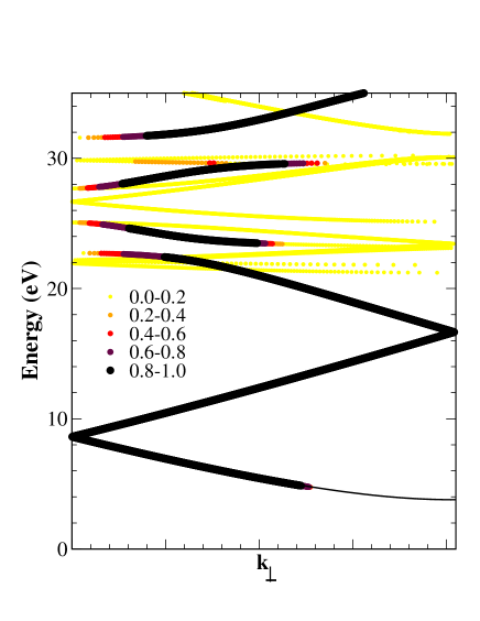
Figure 6: Transmission intensity plotted on top of the unoccupied electron bands along ${k_{\perp}}$ direction for Cu(111). Symbol size and color coding for transmission intensity is given in the legend. The Fermi level is at zero energy.

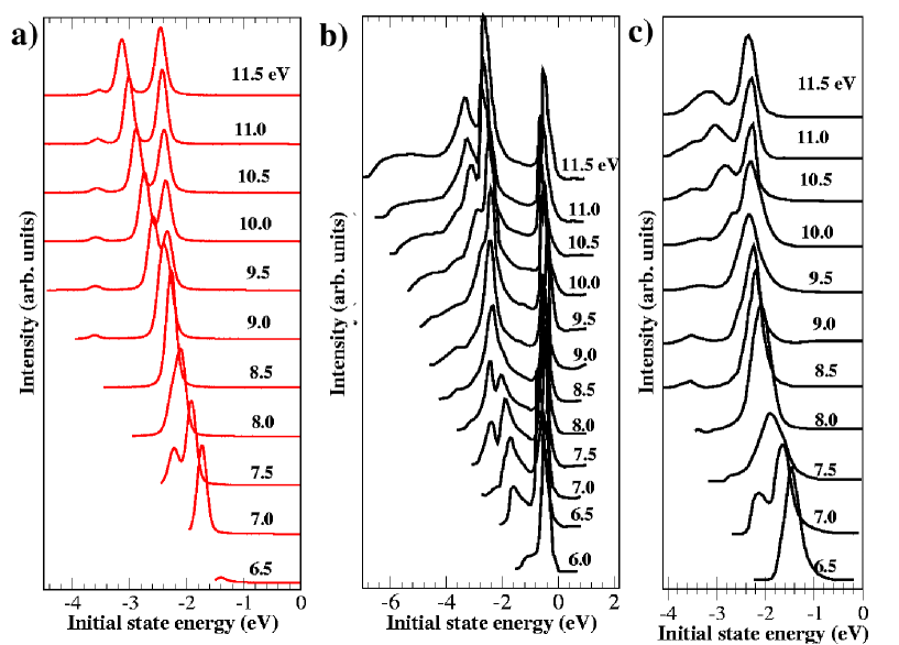
Figure 7: (Color online) In panel a) we present our calculated photoemission spectra from Cu(111), while experimental spectraKnapp et al. (1979) are in panel b). Previous theoretical spectra Smith et al. (1980) are in panel c).

In Fig. 7 we compare our calculated, experimentalKnapp et al. (1979) and previous theoreticalSmith et al. (1980) photoemission spectra from Cu(111) for various photon energies indicated on the figure. Our calculated spectra include the $\epsilon(\omega)$ and LDA+$U$-corrections. The angle of incidence was $60^{\circ}$ and the experiment was performed with 90 % $p$-polarized light. The previous calculations were done within the three-step formalism,D.Grobman et al. (1975) using an empirical band structure generated by the combined-interpolation-scheme approach.Blo In those calculations, the authors decided to additionally suppress the $A_{z}$ contributions to the spectra, in order to get better agreement with the experiment. Our intensities are not adjusted, beyond the corrections imposed by Snell’s law and Fresnel’s equations. Using the bulk-only model, we cannot reproduce the surface peak present in the experimental spectra at about $-0.5$ eV, which is missing also in the previous calculation.Smith et al. (1980) However, our spectra show overall similarity to the experimental spectrum, especially considering the very general trends of changing peak positions and intensities, with increasing photon energy. In comparison with the previous calculation,Smith et al. (1980) two spectra seem to be shifted by 0.5 eV in photon energy, i.e. our spectrum for $\hbar\omega=7.5$ eV is very similar to the one in Ref. Smith et al., 1980 for $\hbar\omega=7.0$ eV. Furthermore, the emergence of the first bulk peak, originating from the $\lambda_{1}$ band at $\hbar\omega=6.5$ eV, (reduced in intensity in our calculation because of an overestimation of the work function), and its shift to the deeper energies for increasing photon energy by 0.5 eV, with a larger weight on the lower states, corresponds to the experimental spectra. For $\hbar\omega=7$ eV, our spectrum has one $\lambda_{1}$ peak, while the transition from the $\lambda_{3}$ band at lower energy is not seen, because of the overestimated work function. Due to poor experimental resolution, it is not easy to deduce if there are two peaks or one in the experimental spectrum. The $\lambda_{3}$ peak is present in our spectrum for $\hbar\omega=7.5$ eV, which reproduces well the experimental spectrum, regarding both the peak positions and intensity. The previous calculation has larger weight on the $\lambda_{3}$ peak, in contrast to the experiment. The single peak in our spectra for $\hbar\omega=8-9$ eV shifts weight from right to the left shoulder (higher to lower energy) and contains contributions from both $\lambda_{1}$ and $\lambda_{3}$ initial states (which cross at those energies). In experimental spectrum, the same trend is present, but it starts from lower photon energy (7.5 eV) and the spectra for lower photon energies have two peaks. For $\hbar\omega=9.0$ eV, a small peak at lower energy emerges ($\sim-3.1$ eV), which corresponds to the $\lambda_{3}$ band and can be found also in all spectra for higher photon energies. It is present also in the previous calculation and in the experimental spectra, where it emerges at $\hbar\omega=8.5$ eV. Our spectra for $\hbar\omega=9.5-11.5$ eV have correct peak positions, but wrong intensity ratio of peaks, significantly overestimating the lower peak, originating from the $\lambda_{1}$-band, with respect to the higher-energy peak, arising from the $\lambda_{3}$-band. The previous calculations resolved this disagreement by artificially suppressing the $z$-polarized contributions. A likely reason for this disagreement is the neglect of surface effects in the three-step model.

V Conclusions

In this paper we have introduced a new method for the ab initio low-energy photoemission calculations based on the pseudopotentials and plane-waves, which has an advantage in its simplicity and unbiased basis-set, with the possibility to significantly reduce the number of empirical parameters. Our method based on the bulk-emission model results in a reasonable agreement with experiment in the photon energy range up to $\sim 25$ eV. Empirical corrections, including the LDA+$U$ and surface-optics, give significant improvements. Nevertheless, in comparison with the one-step model, the intensity ratios of the photoemission peaks are still not fully reproduced. This is due to the neglect of surface damping in our model, which, in principle, could be accounted for within our approach. With respect to the experiment, some broad structures are absent in our spectra, which we interpret to originate from the forbidden transitions in the normal photoemission, caused by the detector’s finite-acceptance angle and the related broadening of ${\bf k_{\parallel}}$. Further work in this direction, i.e. consideration of off-normal photoemission, is necessary to assess these effects.