CMC tori of revolution in : additional data on the spectra of their Jacobi operators
Abstract.
We prove a theorem about elliptic operators with symmetric potential functions, defined on a function space over a closed loop. The result is similar to a known result for a function space on an interval with Dirichlet boundary conditions. These theorems provide accurate numerical methods for finding the spectra of those operators over either type of function space. As an application, we numerically compute the Morse index of constant mean curvature tori of revolution in the unit -sphere , confirming that every such torus has Morse index at least five, and showing that other known lower bounds for this Morse index are close to optimal.
1. Introduction
Our goal is to study the Morse index of constant mean curvature (CMC) tori of revolution in the spherical -space , where the Morse index is the number of negative eigenvalues of the Jacobi operators of those surfaces. The central tool we use is a result about the number of nodes of eigenfunctions of those Jacobi operators. The result, proven with the standard Sturm comparison technique in ordinary differential equations and closely related to classically known results, is proven here before being applied to the index of CMC surfaces of revolution in . So let us start by considering an operator of the form
on function spaces over a closed loop or over an interval with Dirichlet boundary conditions:
We assume the potential function is real-valued and real-analytic on the closed interval , and when the function space is used. However, we do not assume is in when the function space is used, that is, we do not assume and are zero.
The eigenvalue problem is to find and (or ) that solve the second-order ordinary differential equation (ODE)
| (1.1) |
The operator is elliptic and it is well-known ([2], [3], [12], [19]) that the eigenvalues of are real and form a discrete sequence
(each considered with multiplicity 1) whose first eigenvalue is simple. The eigenvalues form a discrete spectrum, and corresponding eigenfunctions
can be chosen to form an orthonormal basis with respect to the standard norm on or over .
Let
denote the domains of the functions in and , respectively. The nodes of an eigenfunction (or ) are those points of (or ) at which vanishes. When is not identically zero, the fact that is second-order and linear implies all zeros of are isolated and of lowest order, i.e. if , then .
We have the following two theorems, the second of which uses a symmetry condition on . The first theorem is well-known and can be proven using Sturm comparison and Courant’s nodal domain theorem (see [5], [6], [7], [8], for example):
Theorem 1.1.
Consider the operator on the function space of functions over with Dirichlet boundary conditions. Then all eigenspaces are -dimensional, and to find a nonzero solution of for some eigenvalue , without loss of generality we may assume:
Furthermore, any eigenfunction associated to the ’th eigenvalue of has exactly nodes.
The following theorem can be similarly proven, but is a bit more complicated, because in this case the eigenvalues are not always simple. We will prove Theorem 1.2 here (and in the process also prove Theorem 1.1). The conclusions about the initial conditions in these two theorems are quite trivial; it is the conclusions about the number of nodes of the eigenfunctions that are of the most interest to us.
Theorem 1.2.
Consider the operator on the function space of periodic functions over . Suppose the real-analytic function has the symmetry
| (1.2) |
Let be the spectrum of with a corresponding basis of eigenfunctions. Then the eigenspaces are each at most -dimensional, and to find a basis for the eigenspace associated to , we may assume:
-
•
When the eigenspace for is -dimensional, we may take so that one of
-
•
When the eigenspace for is -dimensional, and , we may take
Furthermore, any eigenfunction in associated to has exactly nodes if is even, and nodes otherwise.
After proving these results in Section 2, we will see in Section 3 that Theorem 1.2 gives a method to numerically compute the spectra of the operator . Then, in Section 4, we apply that method to study the index of CMC surfaces of revolution in the round -sphere.
In [13], a method was given for computing the eigenvalues for the Jacobi operator of a Wente torus, involving the Rayleigh-Ritz method and restricting to finite dimensional subspaces of function spaces defined over tori. Then in [14], both this method and a second more direct method were given for computing the first eigenvalue of the Jacobi operator of a Delaunay surface with respect to periodic functions, and the second method depended on Delaunay surfaces being surfaces of revolution. It was argued in [14] that, although the second method was clearly the simpler of the two, the first method was still of value because it could compute any eigenvalue of the Jacobi operator, while the second method computed only the first eigenvalue. However, via Theorem 1.2, the second method in [14] in fact extends to a method that gives any eigenvalue and hence is both simpler and equally as robust as the first method. Additionally, this extended second method involves only using any standard ODE solver, such as the Euler algorithm or the Runge-Kutta algorithm, and so has only as much numerical error as those algorithms have, whereas the first method involves restrictions to finite dimension subspaces for which the numerical error cannot be easily estimated and appears to be very much larger than for the extended second method. (This can be seen by comparing the respective errors of the two methods in cases where the spectra are explicitly known.)
Certainly the first method was necessary in [13], because Wente surfaces are not surfaces of revolution. But for the above reasons, the method we give here is in every way superior to the methods found in [13] and [14], in the case of CMC surfaces of revolution.


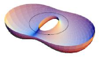
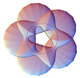
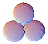
A surface of revolution in the unit 3-sphere is generated by revolving a given planar curve about a geodesic line in the geodesic plane containing this given curve. The given curve is called the profile curve and the geodesic line is called the axis of revolution. The profile curves of non-spherical non-flat CMC surfaces of revolution in will periodically have minimal and maximal distances to the axis of revolution [9]. We call the points of minimal distance the necks, and the points of maximal distance the bulges. In general, when these surfaces close to become compact surfaces without boundary, they are of the following 3 types:
-
•
round spheres, every point of which is the same distance from a fixed point (the center),
-
•
flat CMC tori, every point of which is the same distance from a closed geodesic (the axis of revolution),
-
•
non-flat CMC tori, where the distances from the axis of revolution to the necks and bulges are not equal.
Because these surfaces are closed, the number of negative eigenvalues of their Jacobi operators, counted with multiplicity and called the Morse index, is finite. The Morse index is of interest because it is a measure of the degree of instability of the surface. In the first two cases above, the Morse index is easily explicitly computed [16], being for the first case (this is closely related to the fact that spheres are stable [1]) and always at least for the second case. Regarding the third case, the authors proved the following in [16]:
Theorem 1.3.
Let be a non-flat closed CMC torus of revolution in , with bulges and necks. Let denote the wrapping number of the projection of a profile curve of to the axis circle of revolution. Then:
-
•
has index at least .
-
•
If is nodoidal with , then has index at least .
-
•
If is unduloidal with , then has index at least .


The numerical results here show the lower bounds in the above theorem are very close to the true value for the Morse index in the case of unduloids. For example, using Table 1 and Lemma 4.2, the numerically computed index of the unduloid (resp. , , …, ) is (resp. , , , , , , , , , , , , , , , ), while the above theorem gives the lower bound (resp. , , , , , , , , , , , , , , , ) for the index. In all cases, the lower bound in Theorem 1.3 differs from the numerically computed value for the index by only , thus the lower bound is quite sharp.
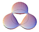
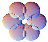
The lower bounds in Theorem 1.3 are not as sharp in the case of nodoids, but still are greater than half of the numerically computed value for all of the surfaces shown in Figure 2. The numerically computed index of the nodoid (resp. , , …, ) is (resp. , , , , , , , , , ), while the above theorem gives the lower bound (resp. , , , , , , , , , ) for the index.
2. Proofs of the Theorems 1.1 and 1.2.
To prove Theorems 1.1 and 1.2, we give a series of lemmas. We first note that:
-
•
For each , it is easily shown that the space of solutions of (1.1) amongst functions is -dimensional.
-
•
Consider the eigenvalue problem (1.1) over the function space on the interval with Dirichlet boundary conditions. Suppose and are two linearly independent eigenfunctions corresponding to some eigenvalue . Noting that and are both nonzero, take the linear combination . Then , and it follows that is identically zero, contradicting the linear independence of and . Hence the eigenvalues are simple. Hence the eigenvalues are always simple for the Dirichlet eigenvalue problem. Furthermore, multiplying by a scalar factor if necessary, we may assume the initial conditions for an eigenfunction is and .
For the closed eigenvalue problem (1.1) with , the eigenspace associated to any eigenvalue is either or dimensional, and we have the following lemma regarding the initial conditions to find a basis for the eigenspace:
Lemma 2.1.
Suppose has the symmetry (1.2). Let be the spectrum of over the space with a corresponding basis of eigenfunctions. Then the eigenspaces are each at most -dimensional, and to find a basis for for some eigenvalue , we may assume:
-
•
When the eigenspace for is -dimensional, we may take a single eigenfunction such that
-
•
When the eigenspace for is -dimensional, we may take two eigenfunctions such that
Proof.
First we consider the case of a -dimensional eigenspace. Let be a basis element of this eigenspace. If has neither the symmetry nor , then and would be two linearly independent eigenfunctions with eigenvalue , a contradiction. Hence or for all , and so or . Furthermore, because multiplying by a real constant still gives a solution to (1.1) with , we may assume either or . Hence the first part of the lemma is shown.
For the case of a -dimensional eigenspace, any solution to (1.1) with lies in , hence we can choose a basis with the initial conditions as in the second part of the lemma. ∎
The following lemma is known as Courant’s nodal domain theorem, and the proof, which applies in our setting with either function space or , can be found in [4] (see also [15]).
Lemma 2.2.
(Courant’s nodal domain theorem.) The number of nodes of any eigenfunction for (1.1) in (resp. ) associated to the ’th eigenvalue is at most (resp. ).
Lemma 2.2 may be strengthened using Sturm comparison, as we will see in the course of proving Theorems 1.1 and 1.2.
The following lemma is a slight generalization of a result in [8]:
Lemma 2.3.
Proof.
Multiplying the first equation in (2.1) by and the second equation in (2.1) by , then subtracting the first expression from the second and integrating, we have
| (2.2) |
as here . Multiplying by the scalar if necessary, we may assume for , so and . If is positive everywhere in , then and , contradicting (2.2). Similarly, cannot be negative everywhere in . ∎
Lemma 2.4.
Consider the eigenvalue problem (1.1) on over the interval with Dirichlet boundary conditions, and with corresponding spectrum of simple eigenvalues. Then any eigenfunction associated with has exactly nodes.
Proof.
Denote a nonzero eigenfunction corresponding to eigenvalue by . Lemma 2.2 implies has exactly two nodes (at and ). Assume has exactly nodal domains and let us prove has exactly nodes. From (1.1) we have and . Let be the zeros of in the interval . Since , applying Lemma 2.3, we conclude that must vanish in each the intervals and hence that it has at least nodes. Lemma 2.2 implies it has exactly nodes. ∎
The following lemma is proven in [8]:
Lemma 2.5.
Let and be two linearly independent solutions of Equation (1.1) for the same , and suppose that has two consecutive zeros and such that , then has one and only one zero in .
Proof.
We may assume is positive for all , then we have and . Because and are independent, for . Here for all , so . Hence cannot keep a constant sign throughout the interval , i.e. has at least one zero in .
Now suppose and are two zeros of in . If we interchange the roles of and in the above argument, we conclude that has at least one zero in , a contradiction. Hence has exactly one zero in . ∎
Lemma 2.6.
Any two eigenfunctions of (1.1) in associated with equal eigenvalues have the same number of nodes.
Proof.
Let and be two eigenfunctions associated with in the spectrum of over . If and are linearly dependent, then the lemma clearly holds, so we assume they are linearly independent.
Suppose has nodes . Then for , and by Lemma 2.5, has a unique node in each of , , …, and . Hence has exactly nodes. ∎
Lemma 2.7.
Take as in Theorem (1.2). Let and in be two eigenfunctions of corresponding to eigenvalues and with , and with either of the initial conditions as in Lemma (2.1). Let and denote the number of nodes in of and , respectively. If and have the same initial conditions, resp. different initial conditions, then , resp. .
Proof.
Suppose , . So has nodes between and . Then by Lemma 2.3, has at least nodes in the open interval , and so . Since and are both even, .
Now suppose , , then has nodes in the open interval . Also, and have the symmetry and for all , by the symmetry (1.2). By Lemma 2.3, has a node in each interval for . Also, it has a node in , so by the above symmetry, it has at least two nodes in , implying and so .
If and have different initial conditions, then Lemma 2.3 immediately implies . ∎
Lemma 2.8.
Proof.
3. Computation of the spectrum of over with symmetric
A numerical method for computing the spectrum of on the function space is as follows:
-
(1)
The eigenfunctions are in and so are periodic, and the real-analytic is assumed to have the symmetry (1.2). Theorem 1.2 implies we can numerically solve (1.1) for with the initial conditions just either , or , by a numerical ODE solver, and search for the values of that give periodic solutions , i.e. give . Such values of are amongst the .
-
(2)
By Theorem 1.2, we know the eigenspaces are at most -dimensional. If, for some , one of the two types of initial conditions in Theorem 1.2 for gives a solution and the other does not, then the eigenspace of is -dimensional; if both types of initial conditions give solutions , then the eigenspace of is -dimensional.
-
(3)
From Theorem 1.2, we know that any eigenfunction associated to has exactly nodes when is even, and nodes otherwise. So the value of is determined simply by counting the number of nodes of . Because we can determine , we will know when we have found all for any given .
4. Application to CMC surfaces of revolution in
| surface | nonpositive eigenvalues (where and ), for the operator |
|---|---|
| -1.28, -1, -1, -0.25, 0 | |
| -1.08, -1, -1, -0.76, -0.76, -0.51, 0 | |
| -1.04, -1, -1, -0.87, -0.87, -0.67, -0.67, -0.52, 0 | |
| -1.03, -1, -1, -0.91, -0.91, -0.78, -0.78, -0.6, -0.6, -0.48, 0 | |
| -1.02, -1, -1, -0.94, -0.94, -0.84, -0.84, -0.714, -0.714, -0.57,-0.57,-0.48, 0 | |
| -1.64, -1.48, -1.48, -1, -1,-0.36, 0 | |
| -1.13, -1.1, -1.1, -1, -1, -0.84, -0.84, -0.64, -0.64, -0.5, 0 | |
| -1.05, -1.04, -1.04, -1, -1, -0.94, -0.94, -0.86, -0.86, -0.77, -0.77, -0.68, -0.68, -0.64, 0 | |
| -1.029, -1.022, -1.022, -1, -1, -0.96, -0.96, -0.92, -0.92, -0.86, -0.86, -0.79, -0.79, -0.72, -0.72, -0.66, -0.66, -0.63, 0 | |
| -1.28, -1.25, -1.25, -1.15, -1.15, -1, -1, -0.83, -0.83, -0.72, 0 | |
| -1.11, -1.1, -1.1, -1.06, -1.06, -1, -1, -0.92, -0.92, -0.83, -0.83, -0.75, -0.75, -0.71, 0 | |
| -1.04, -1.03, -1.03, -1.02, -1.02, -1, -1, -.97, -.97, -0.94, -0.94, -0.896, -0.896, -0.85, -0.85, -0.8, -0.8, -0.76, -0.76, -0.73, -0.73, -0.72, 0 | |
| -1.14, -1.13, -1.13, -1.1, -1.1, -1.06, -1.06, -1, -1, -0.94, -0.94, -0.88, -0.88, -0.86, 0 | |
| -1.14, -1.13, -1.13, -1.1, -1.1, -1.06, -1.06, -1, -1, -0.93, -0.93, -0.84, -0.84, -0.75, -0.75, -0.67, -0.67, -0.63, 0 | |
| -1.07, -1.06, -1.06, -1.05, -1.05, -1.03, -1.03, -1, -1, -0.96, -0.96, -0.92, -0.92, -0.87, -0.87, -0.83, -0.83, -0.78, -0.78, -0.75, -0.75, -0.74, 0 | |
| -1.11, -1.1, -1.1, -1.09, -1.09, -1.07, -1.07, -1.04, -1.04, -1, -1, -0.96,-0.96, -0.93, -0.93, -0.9, -0.9, -0.89, 0 | |
| -1.26, -1.25, -1.25, -1.23, -1.23, -1.19, -1.19, -1.14, -1.14, -1.08, -1.08, -1, -1, -0.91, -0.91, -0.81, -0.81, -0.71, -0.71, -0.62, -0.62, -0.59, 0 | |
| -1.26, -1.19, -1.19, -1, -1, -0.85, 0 | |
| -1.42, -1.31, -1.31, -1, -1, -0.696, 0 | |
| -1.43, -1.37, -1.37, -1.22, -1.22, -1, -1, -0.85, 0 | |
| -1.85, -1.76, -1.76, -1.47, -1.47, -1, -1, -0.55, 0 | |
| -1.67, -1.62, -1.62, -1.49, -1.49, -1.27, -1.27, -1, -1, -0.83, 0 | |
| -1.7, -1.67, -1.67, -1.58, -1.58, -1.43, -1.43, -1.22, -1.22, -1, -1, -0.88, 0 | |
| -1.09, -1.08, -1.08, -1.05, -1.05, -1, -1, -0.95, -0.95, -0.93, 0 | |
| -1.47, -1.45, -1.45, -1.39, -1.39, -1.29, -1.29, -1.16, -1.16, -1, -1, -0.84, -0.84, -0.75, 0 | |
| -1.18, -1.176, -1.176, -1.15, -1.15, -1.11, -1.11, -1.06, -1.06, -1, -1, -0.94, -0.94, -0.89, -0.89, -0.87, 0 | |
| -1.31, -1.3, -1.3, -1.29, -1.29, -1.26, -1.26, -1.22, -1.22, -1.18, -1.18, -1.12, -1.12, -1.06, -1.06, -1, -1, -0.94, -0.94, -0.9, -0.9, -0.89, 0 | |
| -1.19, -1.18, -1.18, -1.17, -1.17, -1.15, -1.15, -1.12, -1.12, -1.09, -1.09, -1.05, -1.05, -1, -1, -0.95, -0.95, -0.91, -0.91, -0.89, -0.89, -0.88, 0 |
As an application of the numerical approach described in Section 3, we consider CMC tori of revolution in the unit -sphere and compute the spectra of their Jacobi operators. This gives us a numerical evaluation of the Morse index of these surfaces.
Let be a conformal immersion from the torus to , with mean curvature and Gauss curvature . When is constant, is critical for a variation problem whose associated Jacobi operator is
where is the Laplace-Beltrami operator of the induced metric for some smooth function ( is in fact real-analytic in the application here). We take to be a non-flat CMC torus of revolution.
Let us define
where . Then the eigenvalues of form a discrete sequence whose corresponding eigenfunctions can be chosen to form an orthonormal basis for the norm over with respect to the Euclidean metric . Let
be the spectrum of .
By using Rayleigh quotient characterizations for eigenvalues it can be shown that and will give the same number of negative eigenvalues (counted with multiplicity), although these two operators will have different eigenvalues. Hence we can use either or to find the Morse index of the surface :
Definition 4.1.
The Morse index of is the sum of multiplicities of the negative eigenvalues of with function space the smooth functions from to . Equivalently, it is the sum of the multiplicities of the negative eigenvalues of over the same function space.
| numerical | |||||||||
| surf- | value | ||||||||
| ace | a | for | |||||||
| Ind() | |||||||||


A function can be decomposed into a series of spherical harmonics as follows:
| (4.1) |
where for with the given . The operator on the function space is defined by
and the spectrum
of has all the analogous properties as those of the spectrum for . Furthermore, by uniqueness of the spherical harmonics decomposition, is an eigenfunction of for the eigenvalue if and only if each , , is an eigenfunction of for the eigenvalue . And if is not identically zero, then some will also be not identically zero. Thus we can say:
-
•
is an eigenvalue for the operator if and only if is an eigenvalue for the operator for some .
-
•
For any eigenvalue , , of , with associated eigenfunction , the eigenvalues of associated to the eigenfunctions and , for integers , will be negative.
Furthermore, we can conclude the following:
Lemma 4.2.
We have
Proof.
Let , resp. , denote the eigenspace of solutions of for smooth , resp. for . Then , resp. whenever is not an eigenvalue of , resp. , and is a positive integer otherwise. Then, by the uniqueness of the spherical harmonics decomposition,
∎
Here is a CMC surface of revolution, so, following [16], we can consider
where , , , and , , (we note that is the mean curvature of ) satisfy the conditions and
and is the elliptic function
When , we have unduloidal surfaces. When , we have either nodoidal or unduloidal surfaces (see [16]).
Using the method in Section 3, we can numerically compute the negative eigenvalues of , and can then apply Lemma 4.2 to find Ind(). We do this for the CMC tori of revolution shown in Figures 1 and 2. In [16], it is shown that is an eigenvalue of , and is an eigenvalue of with multiplicity . Since is discontinuous at and , it is crucial to know that both and are eigenvalues of in order to determine Ind(). Furthermore, as the eigenvalue has multiplicity and must be simple, we have . (In the numerical experiments here, we find that is always a simple eigenvalue.)


References
- [1] L. Barbosa, M. do Carmo and J. Eschenburg, Stability of hypersurfaces of constant mean curvature in Riemannian manifolds, Math. Z. 197 (1988), 123-138.
- [2] P. Berard, Spectral Geometry: Direct and Inverse Problems, Lecture notes in Mathematics 1207 (1986).
- [3] M. Berger, P. Gauduchon, E. Mazet, Le Spectre d’une Variete Riemannienne, Lecture Notes in Math. 194 (1971).
- [4] S.-Y. Cheng, Eigenfunctions and nodal sets, Comment. Math. Helvetici 51 (1976), 43-55.
- [5] R. Courant and D. Hilbert, Methods of mathematical physics, Volume I, Interscience publishers, Inc., New York, 1937.
- [6] J. Diedonne, Foundation of Mathematical Analysis, Academic Press, 1960.
- [7] P. Hartman, Ordinary differential equations, John Wiley and Sons, Inc., 1964.
- [8] E. Hille, Lectures on ordinary differential equations, Addison-Wesley publishing company, 1969.
- [9] W. Y. Hsiang, On generalization of theorems of A. D. Alexandrov and C. Delaunay on hypersurfaces of constant mean curvature, Duke Math. J. 49(3) (1982), 485-496.
- [10] W. Y. Hsiang and W. C. Yu, A generalization of a theorem of Delaunay, J. Diff. Geom. 16 (1981), 161-177.
- [11] H. B. Lawson Jr., Complete minimal surfaces in , Ann. of Math. 92(2) (1970), 335-374.
- [12] S. G. Mikhlin, Variational methods in mathematical physics, Pergamon Press (1964).
- [13] W. Rossman, The Morse index of Wente tori, Geometria Dedicata 86 (2001), 129-151.
- [14] W. Rossman, The first bifurcation point for Delaunay nodoids, J. Exp. Math. 14(3) (2005), 331-342.
- [15] W. Rossman, Lower bounds for Morse index of constant mean curvature tori, Bull. London Math. Soc. 34 (2002), 599-609.
- [16] W. Rossman and N. Sultana, Morse index of constant mean curvature tori of revolution in the 3-sphere, preprint, arXiv:math.DG/0605127.
- [17] N. Schmitt, M. Kilian, S-P. Kobayashi, W. Rossman, Constant mean curvature surfaces with Delaunay ends in -dimensional space forms, to appear in J. London Math. Soc.
- [18] N. Sultana, Explicit parametrization of Delaunay surfaces in space forms via loop group methods, Kobe Journal of Mathematics Vol. 22, No. 1-2 (2005).
- [19] H. Urakawa, Geometry of Laplace-Beltrami operator on a complete Riemannian manifold, Progress on Diff. Geometry, Adv. Stud. Pure Math. 22 (1993), 347-406.


