Gaugino Condensation with
a Doubly Suppressed Gravitino Mass

Abstract

Supersymmetry breakdown via gaugino condensation in heterotic string theory can lead to models with a doubly suppressed gravitino mass. A TeV scale gravitino can emerge from a condensate as large as the grand unified scale. We analyze the properties of these models and discuss applications for particle physics and cosmology.

1 Introduction

One of the basic questions in the study of phenomenological properties of string theories concerns the origin of supersymmetry breakdown. A dynamical mechanism like (hidden sector) gaugino condensation [1, 2, 3] can explain a hierarchically small scale for the gravitino mass

$$m_{3/2}\sim\frac{\Lambda^{3}}{M_{\texttt{P}}^{2}},$$ (1)

where $\Lambda$ denotes the renormalization group invariant scale of the hidden sector gauge group and $M_{\texttt{P}}$ is the Planck mass. In a recent paper [4], Derendinger, Kounnas and Petropolous (DKP) identified a new solution in the framework of the heterotic theory with an even stronger (quadratic) suppression of the gravitino mass

$$m_{3/2}\sim\frac{\Lambda^{6}}{M_{\texttt{P}}^{5}}.$$ (2)

It was discovered in the study of moduli stabilization in the $\mathbbm{Z}_{2}\times\mathbbm{Z}_{2}$ orbifold with NS-NS 3-form and geometric fluxes. While these fluxes (combined with the gaugino condensate) are sufficient to stabilize all moduli in many cases, they fail to do so in the new DKP-solution with the double suppression of the gravitino mass. Two more moduli have to be stabilized and it remains to be seen whether the doubly suppressed solution survives in the process of moduli stabilization.

In the present paper, we try to study the new solution of DKP in a set-up with all moduli fixed, define the criteria for the appearance of this solution and analyze its phenomenological properties. In the next chapter we shall present the model of DKP in its original form and notation. Chapter 3 addresses some shortcomings of the model due to the presence of unfixed moduli. We conclude that it is mandatory to have all moduli fixed before a meaningful analysis of the phenomenological properties can be performed. In chapter 4 we list the basic requirements for the appearance of DKP-like models and define a benchmark model where questions like the fine-tuning of the vacuum energy and the emerging pattern of the soft supersymmetry breaking term can be addressed. For this class of models we are again led to a kind of mirage pattern as previously identified in [5, 6, 7, 8, 9, 10]. Chapter 5 is devoted to applications of this new solution. This includes (most importantly) scenarii with a TeV-scale gravitino and a condensation scale as large as a grand unified scale $M_{\texttt{GUT}}$ or the compactification scale $M_{\texttt{COMP}}$. Other possible applications include the generation of the $\mu$-term $(\mu H_{1}H_{2})$ in models with a small gravitino mass, as well as cosmological applications concerning a quintessential axion and the question of axionic inflation.

2 The model of DKP

The analysis and the notation of this section will follow [4]. We will start considering one important phenomenological requirement, namely, moduli stabilization. To understand whether moduli are stabilized or not we have to check the structure of the scalar potential of the theory, so, as a first step, we dedicate this section to the discussion of the possible terms which can appear in the superpotential. We will consider two contributions: fluxes and gaugino condensates.

2.1 Fluxes, moduli and the superpotential

We will confine our discussion to the $\mathbbm{Z}_{2}\times\mathbbm{Z}_{2}$ orbifold compactification of heterotic strings. This compactification setup leads to seven main moduli (including the string dilaton) and $N=1$ supersymmetry. The effective supergravity is the $\mathbbm{Z}_{2}\times\mathbbm{Z}_{2}$ projection of the $N=4$ theory with sixteen supercharges. Extended supersymmetry is not consistent with our phenomenological requirements, since chiral fermions can exist in four dimensions only when $N\leq 1$. For this reason it is mandatory to reduce the amount of supersymmetry and the orbifold truncation does this. Fluxes are introduced by gauging the $N=4$ supergravity [11, 12, 13, 14, 15, 16]: the parameters of the SUGRA theory are the “gauging structure constants” and these are also the flux parameters.

2.1.1 Moduli identification

The identification of the moduli depends on the theory under consideration. For heterotic strings on ${T^{6}/\mathbbm{Z}_{2}\times\mathbbm{Z}_{2}}$, the moduli are the dilaton-axion superfield $S$, the volume moduli $T_{A}$ and the complex structure moduli $U_{A}$, $A=1,2,3$. The index $A$ refers to the three complex planes left invariant by $\mathbbm{Z}_{2}\times\mathbbm{Z}_{2}$. The $N=1$ supersymmetric complexification for these fields is defined naturally in terms of the geometrical moduli $G_{ij}$ (nine fields), the string dilaton $\Phi$ and the components $B_{ij}$ (three fields) and $B_{\mu\nu}\sim a$ of the antisymmetric tensor. The indices $i\,,j$ run over the internal space and $\mu\,,\nu$ are the Minkowski indices. Explicitly, the metric tensor restricted to the plane $A$ is

$$\left(G_{ij}\right)_{A} =\frac{t_{A}}{u_{A}}\left(\begin{array}[]{cc}u_{A}^{2}+\nu_{A}^{2}&\nu_{A}\\ \nu_{A}&1\end{array}\right),$$ (5)

with

$$T_{A}=t_{A}+i\left(B_{ij}\right)_{A},\qquad\qquad U_{A}=u_{A}+i\,\nu_{A},$$ (6)

and

$$e^{-2\Phi}=s(t_{1}t_{2}t_{3})^{-1},\qquad\qquad S=s+ia.$$ (7)

The Weyl rescaling to the four dimensional Einstein frame is $G_{ij}=s^{-1}{\widetilde{G}}_{ij}$. The $\mathbbm{Z}_{2}\times\mathbbm{Z}_{2}$ projection of the $N=4$ theory leads to the scalar Kähler manifold

$$M= \left[\frac{SU(1,1)}{U(1)}\right]_{S}\times\prod^{3}_{A=1}\left[\frac{SU(1,1)}{U(1)}\right]_{T_{A}}\times\prod^{3}_{A=1}\left[\frac{SU(1,1)}{U(1)}\right]_{U_{A}},$$ (8)

with Kähler potential (in the usual string parameterization)

$$K =-\log\left(S+{\overline{S}}\right)-\sum_{A=1}^{3}\log\left(T_{A}+{\overline{T}}_{A}\right)\left(U_{A}+{\overline{U}}_{A}\right).$$ (9)

It is our intention, on the one hand, to identify the components of the $B$-field which give the imaginary part of the $T$ moduli, on the other hand, to select the possible fluxes which can be “turned on” in this model. The first step is establishing which components of a $p$-form survive the $\mathbbm{Z}_{2}\times\mathbbm{Z}_{2}$ truncation. With this purpose in mind, let us write a generic $p$-form $\omega$ (for a review see [17]) as

$$\omega =\omega_{i_{1},...,i_{p}}dx^{i_{1}}\wedge...\wedge dx^{i_{p}},$$ (10)

where the coordinates $x^{i}$ are subject to the action of the orbifold as summarized in tab. 1. A component of a 3-form with one “leg” in each torus will certainly survive the truncation. This will reveal itself very useful in the next sections when dealing with the (combined) heterotic fluxes.

	$x^{5}$	$x^{6}$	$x^{7}$	$x^{8}$	$x^{9}$	$x^{10}$
$\mathbbm{Z}_{2}$	$-$	$-$	$-$	$-$	$+$	$+$
$\mathbbm{Z}^{\prime}_{2}$	$+$	$+$	$-$	$-$	$-$	$-$

Table 1: Action of the $\mathbbm{Z}_{2}\times\mathbbm{Z}_{2}$ orbifold on the extra-dimensional coordinates.

2.1.2 Heterotic fluxes

As first recognized in [18, 19, 20, 21], possible fluxes in the heterotic theory are those of the modified NS-NS 3-form $\widetilde{H_{3}}=dB_{2}+\ldots$, where the dots stand for the gauge and Lorenz Chern-Simons terms. There are eight independent real fluxes [11, 12], invariant under the $\mathbbm{Z}_{2}\times\mathbbm{Z}_{2}$ orbifold projection:

$$\widetilde{H}_{579}\,,\;\widetilde{H}_{679}\,,\;\widetilde{H}_{589}\,,\;\widetilde{H}_{689}\,,\;\widetilde{H}_{5710}\,,\;\widetilde{H}_{6710}\,,\;\widetilde{H}_{5810}\,,\;\widetilde{H}_{6810}\,.$$ (11)

Leaving aside a systematic discussion, we just observe that, under the assumption of plane-interchange symmetry, there are four independent parameters (corresponding to gauging structure constants) which give $U$ dependent terms in the superpotential:

$$\widetilde{H}_{579} \leftrightarrow 1,$$

$$\widetilde{H}_{679}=\widetilde{H}_{589}=\widetilde{H}_{5710} \leftrightarrow i\,(U_{1}+U_{2}+U_{3}),$$

$$\widetilde{H}_{689}=\widetilde{H}_{5810}=\widetilde{H}_{6710} \leftrightarrow-(U_{1}\,U_{2}+U_{2}\,U_{3}+U_{1}\,U_{3}),$$

$$\widetilde{H}_{6810} \leftrightarrow-i\,U_{1}\,U_{2}\,U_{3}.$$ (12)

The possible fluxes also include some geometrical ones [13, 14, 15, 16], associated with the internal components of the spin connection $\omega_{3}$, and corresponding to coordinate dependent compactifications [22]. These fluxes are characterized by real constants with one upper curved index and two lower antisymmetric curved indices

$$f^{i}_{\;\;jk} =-f^{i}_{\;\;kj}\,.$$ (13)

These constants must satisfy the Jacobi identities of a Lie group, $f^{i}_{\;\;jk}\ f^{k}_{\;\;lm}+f^{i}_{\;\;lk}\ f^{k}_{\;\;mj}+f^{i}_{\;\;mk}\ f^{k}_{\;\;jl}=0$, and the additional consistency condition $f^{i}_{\;\;ik}=0$ [11, 12].

In agreement with the $\mathbbm{Z}_{2}\times\mathbbm{Z}_{2}$ orbifold projection, we must assume here that

$$f^{i_{A}}_{\quad i_{B}i_{C}}=0\qquad{\rm for}\;\;\;\;A=B\;\;{\rm or}\;\;A=C\;{\rm or}\;\;B=C\,,$$ (14)

which satisfies automatically the consistency condition $f^{i}_{\;\;ik}=0$. Geometrical fluxes are then described by 24 real parameters

$$f^{i_{A}}_{\quad i_{B}i_{C}}\,,\qquad\big{[}(ABC)=(123),(231),(312)\big{]}\,,$$ (15)

subject only to the Jacobi identities. The possible structures in the superpotential are $T$ dependent in the form

$$\omega_{i_{B}i_{C}}^{i_{A}}\leftrightarrow iT_{A},T_{A}U_{B},\,iT_{A}U_{B}U_{C},\,T_{A}U_{1}U_{2}U_{3}.$$ (16)

Before proceeding with the analysis, one comment regarding the compactification manifold is necessary. When we switch on fluxes, we are led to heterotic theory on non-Calabi-Yau manifold. In a modern language we can say that e. g. “half-flat” manifolds are exploited implicitly in the DKP model. The existence of these manifolds is strongly suggested by type II mirror symmetry and, recently, heterotic theory on half-flat has been discussed in [23], where a Gukov-type formula has been obtained for the superpotential induced by fluxes. In other words, the flux contribution to the DKP-superpotential can be understood as a Gukov-type formula on a half-flat manifold.

It is also important to recall that, in the heterotic theory, $\widetilde{H}_{3}$ and $\omega_{3}$ fluxes can never generate an $S$-dependent perturbative $N=1$ superpotential. Consequently, if our intention is to stabilize all moduli, including the dilaton, some additional stabilizing contribution must be included. For this reason we will therefore consider nonperturbative effects, in particular, gaugino condensation. For further details on fluxes in heterotic theory the reader is referred to the literature [24, 23, 25, 26, 27].

2.2 Supersymmetry breaking in Minkowski space

In a general supergravity theory with Kähler potential $K=-\sum_{j}\log(Z_{j}+\overline{Z}_{j})$ where $Z_{j}$ denotes the moduli, supersymmetry is spontaneously broken if the equations

$$F^{j}\equiv W-\left(Z_{j}+\overline{Z}_{j}\right)W_{j}=0$$ (17)

cannot be solved for all scalar fields $Z_{j}$ (and with $\real Z_{j}>0$). DKP make a specific ansatz demanding broken supersymmetry in Minkowski space, which implies

$$\langle V\rangle=0\,,\qquad\langle W\rangle\neq 0\,.$$ (18)

A stationary point is found from $\partial_{j}V=0$, $\forall j$, which explicitly reads

$$0=e^{-K}VK_{j}-\overline{W}_{j}F^{j}-3W_{j}\overline{W}+\sum_{i\neq j}\left[W_{j}-\left(Z_{i}+\overline{Z}_{i}\right)W_{ij}\right]\overline{F}^{i}-\left(Z_{j}+\overline{Z}_{j}\right)W_{jj}\overline{F}^{j}\,,$$ (19)

for each scalar field $Z_{j}$. The first term vanishes in Minkowski space and the second derivative of the superpotential $W_{jj}$ is nonzero only for the moduli appearing in the exponential gaugino condensate.

The requirements eq. (18) split the scalar fields into two categories, with either $\langle W_{j}\rangle=0$ and $\langle F^{j}\rangle\neq 0$ or $\langle F^{j}\rangle=0$. Only the first category is involved in SUSY breaking. Tab. 2 shows the field content of each category. Taking this partition of the fields into account, the stationary point condition eq. (19) breaks down to seven conditions

$$0=\sum_{i\neq j}\langle W_{ij}\real Z_{i}\rangle,$$ (20)

with summation restricted over moduli which break supersymmetry.

	$\left\langle W_{j}\right\rangle=0$	$\left\langle F_{j}\right\rangle=0$
Fields	$T_{1}$, $T_{2}$, $T_{3}$	$S$, $U$
SUSY	$+$	$-$

Table 2: Categories of fields in the DKP model.

2.3 The double suppression of the gravitino mass

Consider for concreteness a superpotential of the type [4]

$$W =3\widehat{A}U+\widehat{D}U_{4},$$ (21)

where $U_{4}=U^{3}$. We have introduced the following functions of $T_{1},T_{2}$ and $S$:

$$\widehat{A} =\Big{[}\alpha+\alpha^{\prime}w(\widetilde{S})\Big{]}\xi+Aw(\widetilde{S}),$$ (22)

$$\widehat{D} =\Big{[}\delta+\delta^{\prime}w(\widetilde{S})\Big{]}\xi+Dw(\widetilde{S}),$$ (23)

with $\xi=T_{1}-T_{2}$ and $w(\widetilde{S})=\mu^{3}e^{-\widetilde{S}}=\Lambda^{3}$ where $\mu\simeq M_{\texttt{P}}$ is the RG scale, $\Lambda$ is the RG invariant scale of the confining gauge group and

$$\frac{24\pi^{2}S}{b_{0}} \longrightarrow\widetilde{S}$$ (24)

where $b_{0}$ is the one-loop beta function coefficient.

The minimization condition (20) reads $\real\xi=0$. We will therefore choose $\widetilde{S}=\widetilde{s}-i{\pi/2}$ and $U=u$ real. Everything is consistent provided $\alpha,\delta$ and $A,D$ are real and $\alpha^{\prime},\delta^{\prime}$ are imaginary.

The no-scale requirement $\langle V\rangle=0$ is fulfilled provided $\langle W_{T_{1}}\rangle=\langle W_{T_{2}}\rangle=0$ ($W$ is independent of $T_{3}$) and $F^{S}=F^{U}=0$. This allows us to express $\xi$ and $u$ as functions of $s$. In particular

$$u(\widetilde{s}) =\sqrt{\frac{\widehat{A}}{\widehat{D}}},$$ (25)

$$\xi(\widetilde{s}) =-\frac{1}{4}\frac{3D\alpha+A\delta+\left(3D\alpha^{\prime}+A\delta^{\prime}\right)w}{\left(\alpha+\alpha^{\prime}w\right)\left(\delta+\delta^{\prime}w\right)}w.$$ (26)

The central equation for the determination of $\widetilde{s}$ is given by:

$$\frac{~{}2~{}}{\widetilde{s}} =-4-\frac{\left(\alpha^{\prime}\delta-\delta^{\prime}\alpha\right)w}{\left(\alpha+\alpha^{\prime}w\right)\left(\delta+\delta^{\prime}w\right)}\frac{3D\alpha+A\delta+\left(3\alpha^{\prime}D+A\delta^{\prime}\right)w}{D\alpha-A\delta+\left(D\alpha^{\prime}-A\delta^{\prime}\right)w}.$$ (27)

As previously discussed in [4], eq. (27) admits physically acceptable solutions for $\widetilde{s}$, provided that the fluxes $\alpha,\delta,\alpha^{\prime},\delta^{\prime},A,D$ are large while their ratios are of order unity. If this requirement is fulfilled we can define a variable $\rho$ (real function of $\widetilde{s}$) as

$$\rho=i\frac{D\alpha-A\delta}{D\alpha w},$$ (28)

which can be consistently taken to be of order one since $w$ is small and $D\alpha/A\delta$ is of order one. As we shall discuss later, this requires a certain amount of fine tuning for $D\alpha-A\delta\ll 1$.

The gravitino mass is given by [4]:

$$e^{-K/2}m_{3/2} =\langle W\rangle$$

$$=\frac{A\delta^{\prime}-D\alpha^{\prime}+\frac{A\delta-D\alpha}{w}}{\alpha+\alpha^{\prime}w}\left(-3\frac{\alpha+\alpha^{\prime}w}{\delta+\delta^{\prime}w}\right)^{3/2}w^{2}\,,$$ (29)

for generic plane symmetric situations. In the special case $\alpha^{\prime}=i\alpha$ and $\delta^{\prime}=-i\delta$ and within the above approximations, the result is

$$e^{-K/2}m_{3/2} \approx i\left(2De^{-2\widetilde{s}}+\frac{A\delta-D\alpha}{\alpha}e^{-\widetilde{s}}\right)$$

$$\approx i4D\left(-\frac{3\alpha}{\delta}\right)^{3/2}\frac{\widetilde{s}}{2\widetilde{s}+1}w^{2}.$$ (30)

The gravitino mass scales as $w^{2}$ and this is due to the absence of flux-induced $S$-term in the heterotic superpotential.

It is relevant to discuss which values of the parameters will give a small $w$. If we consider a Planckian scale $\mu$ then $\widetilde{s}\sim 10$ is necessary to have a small $w$ and to achieve a reasonable value of $g_{\texttt{GUT}}$. Eq. (30) written in the form shows that the $S$ modulus is stabilized through the presence of the condensate. Strictly speaking, this is not a “racetrack” mechanism proper [28] because we only have one condensate. However, the condensate enters into the superpotential in a rather complex way and several terms are added together, so, as far as our model is concerned, it gives a result that otherwise can only be achieved by a racetrack mechanism.

3 Problematic aspects of the model

Up to now the stabilization of the moduli can be summarized as follows:

• $S$ can be stabilized at an acceptable value,

• $U$ is real and stabilized through fluxes,

• $\xi=T_{1}-T_{2}$ is fixed as a function of $S$ and $\real\xi=0$ from eq. (20),

• $T_{3}$ and $T_{1}+T_{2}$ are flat directions and thus not stabilized.

3.1 Unfixed moduli

The problematic aspect of the DKP-strategy is the appearance of unfixed $T$ moduli. It is a consequence of the restricted no-scale ansatz eq. (18) and it leads to a situation with $F^{S}=0$ and $F^{T}\neq 0$. This ansatz requires $E_{\texttt{VAC}}=0$ in a situation where not all moduli are fixed. It remains to be seen whether this strategy is the most appropriate one since the goal of the procedure is a vanishing $E_{\texttt{VAC}}$ after fixing all moduli.

One way to proceed is the application of the old local no-scale idea, where one assumes corrections to the Kähler potential which fix the remaining moduli while keeping $E_{\texttt{VAC}}=0$. Thus to remove the flat directions we will modify the Kähler potential demanding the flatness condition ($V\equiv 0$) only locally [29, 30]. In the remaining part of this section we will focus on this point (following the notation in [29]). The final outcome will be the stabilization of all moduli.

For the flatness condition to be around point $z_{0}$ in $\cal D$ (the positive kinetic energy domain $G_{z\overline{z}}>0$), we demand

$$\partial_{z}\partial_{\overline{z}}e^{-G/3}=\phi_{z\overline{z}}(z,\overline{z}),$$ (31)

where the real function $\phi(z,\overline{z})$ satisfies the conditions

$$\phi_{z\overline{z}}\geq 0,\forall z\in\cal{D}$$ (32)

and

$$\phi_{z\overline{z}}(z_{0},\overline{z}_{0})=0.$$ (33)

The general solution of eq. (31) is

$$G=-\frac{3}{2}\log\left(f+\overline{f}+\phi\right)^{2},$$ (34)

with the positive kinetic energy domain defined by

$$G_{z\overline{z}}=3\frac{\left|f_{z}+\phi_{z}\right|^{2}-\phi_{z\overline{z}}\left(f+\overline{f}+\phi\right)}{\left(f+\overline{f}+\phi\right)^{2}}>0.$$ (35)

The corresponding scalar potential is positive definite in $\cal{D}$, provided that $\phi_{z\overline{z}}\geq 0$ as well as $f+\overline{f}+\phi>0$ as can be seen from its analytic expression

$$V =3\frac{\phi_{z\overline{z}}\left(f+\overline{f}+\phi\right)}{\left|f+\overline{f}+\phi\right|^{3}\left[\left|f_{z}+\phi_{z}\right|^{2}-\phi_{z\overline{z}}\left(f+\overline{f}+\phi\right)\right]}.$$ (36)

The Kähler correction is designed in such a way that it vanishes at $z_{0}$. Thus, the presence of $\phi$ in the scalar potential deforms its shape only outside $z_{0}$. Let us for concreteness consider

$$\phi =\frac{\left(z-z_{0}\right)^{2}\left(\overline{z}-\overline{z}_{0}\right)^{2}}{4},$$ (37)

and apply the analysis to $z=T_{3}$. As evident from eq. (37) we obtain $\phi_{z\overline{z}}=\left|T_{3}-z_{0}\right|^{2}$ and the positivity condition eq. (35) is fulfilled. The scalar potential exhibits a local minimum at $z_{0}$. Fig. 2 illustrates the scalar potential in the complex $T_{3}$ plane. A similar procedure can be exploited to remove the $T_{1}+T_{2}$ flat direction. Note that due to the Kähler correction $\phi$ the Kähler manifold no longer exhibits the $SU(1,1)$ symmetry. In the minimum $z_{0}$, however, the stabilization of $S$ does not clash with the stabilization of $T_{3}$ and $T_{1}+T_{2}$ since in $z_{0}$ the correction $\phi$ and its derivatives vanish.

Figure 1: Scalar potential for the dilaton.

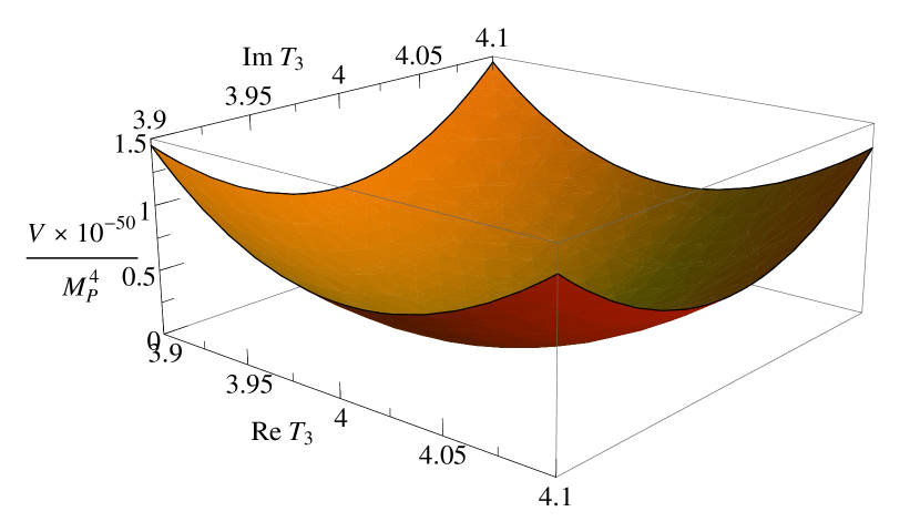
Figure 2: Stabilizing potential for $T_{3}$ displayed in the complex plane.

Since we have stabilized now all the moduli in the presence of broken supersymmetry, we can start to analyze explicitely the resulting pattern of soft supersymmetry breaking terms.

3.2 The pattern of supersymmetry breakdown

3.2.1 Tree-level $\boldsymbol{F}$-terms and $\boldsymbol{m_{3/2}}$

To obtain a phenomenologically attractive gravitino mass we shift the position of the minimum in the $S$ direction to $\widetilde{S}_{0}=15-i\pi/2$. This corresponds, by reversing the rescaling eq. (24), to the gauge group $SU(11)$. We choose the minima in the $T$ directions to be at $T_{0}=4+i4$. A Minkowski vacuum is obtained e. g. for the following set of flux coefficients

$$\alpha=100,\,\delta=-100,\,A=10,\,D=-10.00001.$$ (38)

This choice respects the condition that eq. (28) is of order one and we have a doubly suppressed gravitino mass. In greater detail, numerically $(A\delta-D\alpha)/(\alpha w)\simeq 33$ and we keep under control the dangerous $1/w$ contribution, that could spoil the double suppression in the gravitino mass formula, granted that we accept a mild fine-tuning of the parameters of order $A\delta-D\alpha\simeq 10^{-3}$.

In this particular vacuum we obtain

$$F^{S} =F^{U}=0,$$ (39)

$$F^{T_{1}} =F^{T_{2}}=F^{T_{3}}=-8m_{3/2},$$ (40)

where the gravitino mass is given by $m_{3/2}=1.11\times 10^{-14}M_{\texttt{P}}$. Remarkably the local no-scale structure exploited to stabilize the flat directions does not modify the result $F^{S}=0$. At first sight, the result $F^{T_{1}}=F^{T_{2}}=F^{T_{3}}$ might be surprising since the $T$ moduli have been considered in a strongly asymmetric way in the superpotential and during the process of stabilization. However, we must remember that $W_{T_{1}}=W_{T_{2}}=W_{T_{3}}=0$ was one of the conditions to obtain a Minkowski (no-scale) solution and, once exploited in the evaluation of the $F$ terms, it will give us the very symmetric configuration $F^{T_{1}}=F^{T_{2}}=F^{T_{3}}$.

3.2.2 Tree-level soft terms

For the evaluation of the soft supersymmetry breaking terms we include the contribution of matter fields in the Kähler potential. We will focus our attention on $(0,2)$ symmetric orbifolds. If we denote collectively the $T$ and the $U$ moduli by $T_{p}$, where e. g. $T_{p}=U_{p-3}$ with $p=\{3,4,5\}$, the Kähler potential becomes [32, 33]

$$K =-\log\left(S+\overline{S}\right)-\sum_{p}\log\left(T_{p}+\overline{T}_{p}\right)+\sum_{\alpha}Q_{\alpha}\overline{Q}_{\alpha}\prod_{p}\left(T_{p}+\overline{T}_{p}\right)^{-n^{p}_{\alpha}},$$ (41)

with $Q_{\alpha}$ being the observable matter fields and $n^{p}_{\alpha}$ are the so-called modular weights. As already mentioned before, in our vacuum we have $F^{S}=F^{U}=0$. Consequently the structure of the Kähler potential simplifies to

$$K =-\sum_{i=1}^{3}\log\left(T_{i}+\overline{T}_{i}\right)+\sum_{\alpha}Q_{\alpha}\overline{Q}_{\alpha}\left(T_{1}+\overline{T}_{1}\right)^{-n^{1}_{\alpha}}\left(T_{2}+\overline{T}_{2}\right)^{-n^{2}_{\alpha}}\left(T_{3}+\overline{T}_{3}\right)^{-n^{3}_{\alpha}}.$$ (42)

We evaluate scalar masses, soft trilinear couplings and gaugino masses from (see e. g. [34, 35])

$$m^{2}_{\alpha} =m_{3/2}^{2}-\overline{F}^{m}F^{n}\partial_{m}\partial_{n}\log\mathcal{K_{\alpha}},$$ (43)

$$A_{\alpha\beta\gamma} =F^{m}\left[\widehat{K}_{m}+\partial_{m}\log Y_{\alpha\beta\gamma}-\partial_{m}\log\left(\mathcal{K_{\alpha}}\mathcal{K_{\beta}}\mathcal{K_{\gamma}}\right)\right],$$ (44)

$$M_{a} =\frac{1}{2}\left(\real f_{a}\right)^{-1}F^{m}\partial_{m}f_{a},$$ (45)

where $m$ runs over SUSY breaking fields, $\widehat{K}$ is the Kähler potential for the hidden sector fields, $\mathcal{K_{\alpha}}=\frac{\partial^{2}K}{\partial Q_{\alpha}\partial\overline{Q}_{\alpha}}$ and we will assume that $Y_{\alpha\beta\gamma}$ are moduli independent. We obtain

$$m_{\alpha}^{2} =m_{3/2}^{2}\big{[}1-n^{1}_{\alpha}-n^{2}_{\alpha}-n^{3}_{\alpha}\big{]},$$ (46)

$$A_{\alpha\beta\gamma} =m_{3/2}\Big{[}\left(1-n^{1}_{\alpha}-n^{1}_{\beta}-n^{1}_{\gamma}\right)+\left(1-n^{2}_{\alpha}-n^{2}_{\beta}-n^{2}_{\gamma}\right)+\left(1-n^{3}_{\alpha}-n^{3}_{\beta}-n^{3}_{\gamma}\right)\Big{]},$$ (47)

$$M_{a} =0,$$ (48)

where $n_{\alpha}^{1}+n_{\alpha}^{2}+n_{\alpha}^{3}=1$. At tree-level we have really a no-scale configuration for the soft terms: the scalar masses, the trilinear couplings and the gaugino masses are vanishing.

3.2.3 Quantum corrections

In the previous section we obtained vanishing tree-level soft terms. To construct a realistic model we can take into account quantum effects like anomaly mediation [36] and/or threshold corrections to the gauge kinetic function [37, 38, 39, 40]. However, since loop corrections exceedingly complicate the evaluation of the soft terms, we will dedicate the next section entirely to the discussion of a simple benchmark model encompassing the main features of the DKP set-up. In this section instead, we will summarize the modifications induced by threshold corrections in our model (in the gauge kinetic function, in the superpotential and in the Kähler potential).

The detailed structure of quantum corrections depends on the model we consider (the case of $\mathbbm{Z}_{2}\times\mathbbm{Z}_{2}$ orbifold model is discussed in [41, 42, 43]) and usually these corrections are complicated functions of the moduli [37, 38, 39, 40]. However for our purposes it will be sufficient to consider the following modification to the gauge kinetic function (see [44])

$$f=S+\epsilon T,$$ (49)

where the explicit $T$ dependence will lead us to nonvanishing gaugino masses and $\epsilon$ is a small number that we now specify. The one-loop gauge coupling constant is given by the real part of a gauge kinetic function of the form [45]

$$f_{\texttt{1-LOOP}}=S-\frac{1}{8\pi^{2}}\sum_{i}\left(\frac{b_{0}}{3}-\delta_{\texttt{GS}}^{i}\right)\log\eta^{2}(T_{i}),$$ (50)

where $b_{0}$ is a beta function coefficient and the mixing with coefficient $\delta_{\texttt{GS}}^{i}$ generalizes the Green-Schwarz mechanism. For large $T$ we have $\log\eta(iT)\sim-\frac{\pi}{12}T$, and in our $\mathbbm{Z}_{2}\times\mathbbm{Z}_{2}$ orbifold model $\delta_{\texttt{GS}}^{i}=0$ [46]. In this way we recover the simpler structure of eq. (49).

The superpotential of the model contains the nonperturbative factor $w(\widetilde{S})=e^{-\widetilde{S}}$ which depends crucially on the value of the gauge coupling constant $g$. At loop-level $g$ is not specified only by the dilaton field $S$, but also by the $T$ field. For this reason we will substitute the $S$ field in the superpotential with the 1-loop corrected expression $S+\epsilon T$ (see above).

In case of a pure Yang-Mills theory, the one-loop Kähler potential is given by [39, 45, 43]

$$K_{\texttt{1-LOOP}}=-\log\left[\left(S+\overline{S}\right)-\frac{1}{8\pi^{2}}\sum_{i=1}^{3}\delta_{\texttt{GS}}^{i}\log\left(T_{i}+\overline{T}_{i}\right)\right]-\sum_{i=1}^{3}\log\left(T_{i}+\overline{T}_{i}\right).$$ (51)

$K_{\texttt{1-LOOP}}$ now leads to a mixing between the $S$ and the $T_{i}$ fields, but in our orbifold model $\delta_{\texttt{GS}}^{i}$ is vanishing and no correction will be present [46].

This mixing of $S$ and $T$ will induce soft supersymmetry breaking terms in the observable sector, including nontrivial gaugino masses. Of course, the mixing will also induce a shift in the location of the minimum of the effective potential. Such a shift will generically lead to a nonvanishing value of the vacuum energy as well. A further fine tuning is required to obtain a suitable value for $E_{\texttt{VAC}}$. A complete treatment of the effective potential is rather complicated and will not be discussed here in detail. We shall rather adopt a strategy different from DKP in order to simplify the discussion.

3.3 Intermediate conclusions

As we have seen, we can fix the remaining moduli and keep vanishing vacuum energy. The strategy adopted so far, however, has several drawbacks. The corrections to the Kähler potential in eq. (34) are chosen ad hoc and there is no convincing theoretical justification (e. g. from string theory considerations). The procedure is such that $F^{S}=0$ is frozen in and we have problems with the soft supersymmetry breaking terms, e. g. vanishing tree level gaugino masses. It is also well known that radiative corrections spoil the no-scale structure. As we have seen above, generically these corrections induce a mixing of $S$ and $T$ and therefore $F^{S}\neq 0$ as well as a nonvanishing contribution to $E_{\texttt{VAC}}$. Thus the vacuum energy has to be tuned a second time. We therefore conclude that the no-scale strategy of DKP is not necessarily the most appropriate one. One should first fix all moduli (without intermediate assumptions on $E_{\texttt{VAC}}$) and then care about (the tuning of) the vacuum energy once and for all.

This is what we are trying to do in the next chapter. The question is whether the observed double suppression of the gaugino condensate can be realized in this more general set-up as well, or whether it is tied to the specific no-scale ansatz eq. (18) adopted by DKP.

4 Towards a resolution of the problems

4.1 Basic ingredients

Let us recapitulate the basic ingredients needed for the double suppression. The obvious requirement is the absence of $S$ in the perturbative superpotential (only nonperturbative contributions of the form $e^{-S}$ are present) which is automatically fulfilled in the heterotic theory. We also need some tuning of parameters as explained in the last section ($A\delta-D\alpha\ll 1$). One should also note that terms with $e^{-S}$ in the superpotential need to be multiplied by non-trivial functions of the $T$ moduli (a generic result in the heterotic theory originating in world sheet instanton effects [47, 48]). Last but not least we need a superpotential with terms that allow large masses for the $T$ moduli, although the classical superpotential does not include quadratic terms in $T$ (but only constant and linear terms). This requirement has been discussed in detail in [5] both for the heterotic and the type IIB case, and it strongly relies on the existence of the complex structure moduli. Once these have been fixed and integrated out we are left with an effective superpotential $W_{\texttt{EFF}}(S,T)$ which could include terms quadratic (and higher order) in $T$. Of course, one could also consider more general compactification than the $\mathbbm{Z}_{2}\times\mathbbm{Z}_{2}$ orbifolds considered by DKP that allow for more general superpotentials. In any case, the above requirements seem to be quite easily fulfilled in the framework of heterotic string theory.

We thus consider the heterotic theory with $S$, $T$, and $U$ moduli as given in DKP. In a first step we use fluxes to fix the $U$ moduli without breaking supersymmetry. The $U$ moduli become heavy and can be integrated out leading to an effective superpotential $W_{\texttt{EFF}}(S,T)$ where $S$ only appears through the condensate $e^{-S}$. The simplest form to realize the doubly suppressed solution of DKP then reads: $W_{\texttt{EFF}}\sim Te^{-S}+T^{2}$ where we dropped numerical coefficients for the moment. The equation of motion for $T$ then relates $T\sim e^{-S}$ and $\left\langle W_{\texttt{EFF}}\right\rangle\sim(e^{-S})^{2}$ , as desired. The mild fine-tuning of DKP ($A\delta-D\alpha\ll 1$) has a counterpart in our benchmark model: the coefficient of a possible term linear in $T$ has to be small, otherwise the double suppression would be spoiled. Thus this simple model captures all the aspects of the DKP-model with one exception: the $S$ modulus is not yet fixed. In fact, we are faced with a potential that shows run-away behavior for $S\rightarrow+\infty$, and the potential is positive. Therefore we have to find a mechanism to fix $S$ and tune the vacuum energy to an acceptable value. Both problems can be solved simultaneously by adopting the “downlifting strategy” explained in [49]. This will be explicitely worked out in the remainder of this section.

4.2 A benchmark model

Given the guidelines in the previous section the purpose of this part is to construct and analyze a simpler framework covering the key features of the DKP model. The fact that the only $S$-dependence of the superpotential in the DKP model is encoded in the gaugino condensate, can be identified as the crucial requirement for the double suppression. We would like to express the complicated form of the superpotential eq. (21) in a more transparent language. In what follows we consider $S$, $T$ and $U$ moduli. After the $U$ moduli have been integrated out we assume the effective superpotential to be of the form

$$W_{\texttt{EFF}} =\mathcal{A}_{0}e^{-aS}T+\mathcal{A}_{1}T+\mathcal{A}_{2}T^{2}+\cdots+\mathcal{A}_{n}T^{n},$$ (52)

where $\mathcal{A}_{0}$,…,$\mathcal{A}_{n}$ and $a$ are real constants. For the case of simplicity we are considering a real dilaton field $S$ and one single real Kähler modulus $T$. We fine-tune the coefficient $\mathcal{A}_{1}$ to be small (see discussion above) such that the term linear in $T$ becomes negligible.

The equation of motion for the $T$ modulus $F^{T}=0$ reads

$$0 =W\partial_{T}K+\partial_{T}W$$ (53)

$$=\mathcal{A}_{0}\left(-\frac{3}{2}+1\right)e^{-aS}+\mathcal{A}_{2}\left(-\frac{3}{2}+2\right)T+\cdots+\mathcal{A}_{n}\left(-\frac{3}{2}+n\right)T^{n-1}.$$ (54)

For eq. (54) to be satisfied, $T$ has to be small which implies that $T^{3}$ and higher powers of $T$ can be safely neglected in eq. (52). From the equation of motion eq. (54) one obtains

$$T =\frac{\mathcal{A}_{0}}{\mathcal{A}_{2}}e^{-aS}.$$ (55)

Consequently we can integrate out the $T$ field and end up with the effective superpotential

$$W_{\texttt{EFF}} =2\frac{\mathcal{A}_{0}^{2}}{\mathcal{A}_{2}}e^{-2aS}.$$ (56)

This is exactly the double suppression as obtained in the DKP model. At this stage, however, the dilaton is not yet stabilized since the scalar potential from eq. (56) shows a run-away behavior. The remaining task to perform is to stabilize the dilaton and assure a reasonable vacuum energy. As was recently shown [49] these two operations can be done economically in one step.

Following the discussion of [49] we consider the impact of hidden sector matter through the interaction with the effective theory obtained after integrating out $U$ and $T$ moduli. For concreteness and simplicity we will focus on a Polonyi-type superpotential [50] so that the full superpotential is given by

$$W =W_{\texttt{EFF}}(S)+W_{\texttt{POLONYI}}(C)$$

$$=-Ae^{-2aS}+\nu+\tau^{2}C,$$ (57)

where we have chosen $\mathcal{A}_{0}=\mathcal{A}_{2}=-A/2$, $\nu$ and $\tau^{2}$ are constants and $C$ represents a hidden sector matter field, assumed to be a gauge singlet. The corresponding Kähler potential is

$$K =-\log{\left(S+\overline{S}\right)}+C\overline{C}.$$ (58)

As shown in [49], systems of this type are capable of changing the shape of the run-away scalar potential and lead to formation of stationary points. The stationary point in the configuration eq. (57, 58) turns out to be a local minimum. By appropriately choosing the parameters of the Polonyi subsector the cosmological constant can be adjusted/finetuned to the desired value.

The consequence of the $F$-term uplifting/downlifting is the appearance of a so-called little hierarchy [51, 52, 49, 53] originating from the factor

$$\Upsilon=\log{\left(\frac{M_{\texttt{P}}}{m_{3/2}}\right)}\sim\mathcal{O}\left(4\pi^{2}\right).$$ (59)

In particular it leads to a suppression of the dilaton contribution to the soft terms

$$F^{S} \sim\frac{m_{3/2}}{\Upsilon},$$ (60)

such that SUSY breaking is dictated by the matter sector, since $F^{C}\sim m_{3/2}$. The scale of the soft terms is set by the gravitino mass

$$m_{3/2} =e^{K/2}\left|W\right|\sim\tau^{2}$$ (61)

implying that $\tau^{2}$ sets the scale of the gravitino mass (and also the mass of the Polonyi field). However $\tau^{2}\sim\Upsilon e^{-2aS}$, consequently the gravitino mass originates from the gaugino condensation and is doubly suppressed. A concrete realization based on the hidden sector gauge group $SU(8)$ is shown in fig. 4 and tab. 3, summarizing the main parameters.

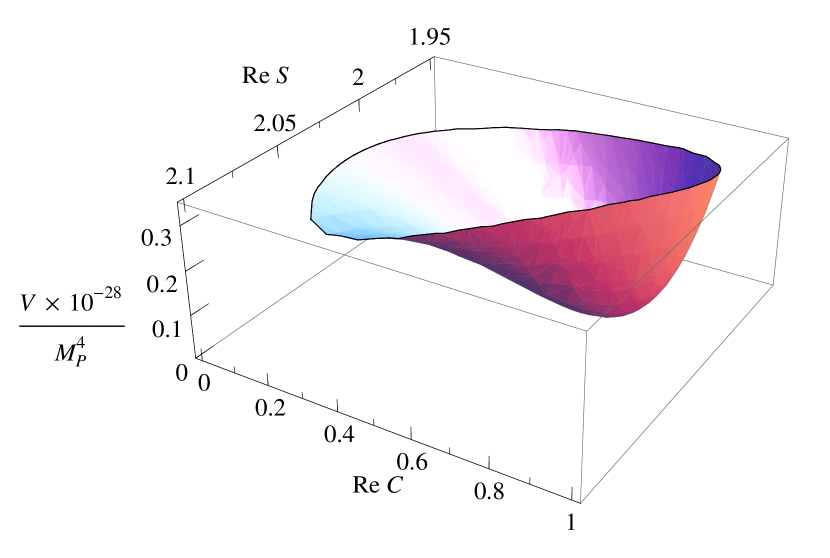
Figure 3: Scalar potential for the $S$-$C$ system.

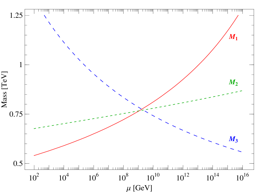
Figure 4: RG evolution of the gaugino masses.

$\nu$	$\tau^{2}$	$C_{0}$	$F^{S}$	$F^{C}$	$m_{3/2}$	$m_{S}$	$m_{C}$
$4\times 10^{-15}$	$2\times 10^{-14}$	$0.73$	$9\times 10^{-16}$	$2\times 10^{-14}$	$25\,\mathrm{TeV}$	$1909\,\mathrm{TeV}$	$43\,\mathrm{TeV}$

Table 3: Sample spectrum with a multi-TeV gravitino for $SU(8)$.

To analyze the structure of the resulting soft terms we focus on the case $C_{0}\ll 1$. Allowing couplings between hidden matter $C$ and observable fields $Q_{\alpha}$ in the Kähler potential

$$K =-\log{\left(S+\overline{S}\right)}+C\overline{C}+Q_{\alpha}\overline{Q}_{\alpha}\Big{[}1+\varsigma_{\alpha}C\overline{C}\Big{]},$$ (62)

the emerging soft terms are given by

$$m^{2}_{\alpha} =\varsigma_{\alpha}\frac{\left|F^{S}\right|^{2}}{\left(S_{0}+\overline{S}_{0}\right)^{2}}+\left(1-3\varsigma_{\alpha}\right)m^{2}_{3/2}+\mathtt{ANOMALY},$$ (63)

$$A_{\alpha\beta\gamma} =-\frac{F^{S}}{S_{0}+\overline{S}_{0}}+\mathtt{ANOMALY},$$ (64)

$$M_{a} =\frac{F^{S}}{S_{0}+\overline{S}_{0}}+\mathtt{ANOMALY},$$ (65)

where “ANOMALY” denotes possible 1-loop and 2-loop contributions to the soft terms. As eq. (60) shows, the dilaton contribution is suppressed by the little hierarchy. Therefore gaugino masses and $A$-terms feel the contribution from dilaton and anomaly in comparable portions in the spirit of a hybrid mediation, also know as mirage mediation [5, 6, 7, 9, 10, 8, 54, 52, 53, 55, 56, 57, 58, 51]. The fate of the soft scalar masses is more model dependent and crucially depends on the parameter $\varsigma_{\alpha}$ which describes the coupling between hidden and observable matter. For $\varsigma_{\alpha}\ll 1$ the dilaton as well as the anomaly contribution are negligible. In this scenario the scalar masses are dominated by the $F$-term of the downlifting field $C$. On the other hand, for $\varsigma_{\alpha}\sim\mathcal{O}(\nicefrac{{1}}{{3}})$ the matter contribution to scalar masses becomes suppressed whereas dilaton and anomaly mediated parts provide comparable contributions.

While one can realize different scenarii for the scalar masses, mirage mediation for the gauginos and the $A$-terms is more reliable and independent of $\varsigma_{\alpha}$. The gaugino masses encode the mirage unification feature in the most robust way [59]. This mirage scale is determined by the relative strength of dilaton versus anomaly mediation in eq. (65). Fig. 4 shows the evolution of the gaugino masses for equal dilaton/anomaly contribution. Finally, the masses of the dilaton, the Polonyi field, the gravitino and the gauginos exhibit the hierarchy

$$m_{S}\sim\Upsilon m_{3/2}\sim\Upsilon m_{C}\sim\Upsilon^{2}m_{1/2}.$$ (66)

5 Applications

Let us try to see how the new scenario with a doubly suppressed gravitino mass can be applied to various aspects of model building in particle physics and cosmology.

5.1 Small gravitino mass with a large $\boldsymbol{\Lambda}$

The standard formula [1] for the gravitino mass from a gaugino condensate reads

$$m_{3/2}\sim\frac{\Lambda^{3}}{M_{\texttt{P}}^{2}}$$ (67)

and $F\sim\Lambda^{3}/M_{\texttt{P}}$. It requires $\Lambda$ to be at an intermediate scale if $m_{3/2}$ is at the (multi) TeV scale. To raise $\Lambda$ in a realistic set-up would require soft terms that are small compared to $m_{3/2}$ [1] and this is not easy to achieve. The doubly suppressed solution gives

$$m_{3/2}\sim\frac{\Lambda^{6}}{M_{\texttt{P}}^{5}},$$ (68)

and avoids an intermediate scale.

In a rather natural way $\Lambda$ could be identified with the grand unified scale $M_{\texttt{GUT}}$ or the compactification scale $M_{\texttt{COMP}}$ of extra dimensions in string theory, typically assumed to be at a scale of few times $10^{16}\,\mathrm{GeV}$. Thus a single scale $\Lambda$ might represent $M_{\texttt{GUT}}\sim M_{\texttt{COMP}}$ as well as the hierarchically small scale $m_{3/2}$. Model building along these limes might be promising.

In our benchmark model we obtained a hidden sector group $SU(8)$ assuming a pure supersymmetric $SU(N)$ gauge theory as well as the equality of the gauge coupling constants of hidden and observable sector. This group could originate certainly from the $SO(32)$ theory but not so easily [54] from the $E_{8}\times E_{8}$ theory favored by phenomenological arguments [60, 61]. String threshold corrections, however, might enlarge the hidden sector gauge coupling compared to the observable sector one, allowing for smaller hidden sector gauge groups and thus reopening many new ways for model building. In fact, in heterotic M-theory [62, 63], a larger coupling in the hidden sector might appear in a natural way [64, 65, 66]. Such models might then explain all scales directly from the string scale, without invoking the existence of an intermediate scale.

5.2 The $\boldsymbol{\mu}$-problem in gauge mediation

If we considered a situation with condensation at the intermediate scale in a model with double suppression we would obtain a rather smallish gravitino mass. SUSY breaking at the weak scale would then need another source, as in models of supersymmetry breakdown via gauge mediation [67, 68, 69] (i. e. the gravitino mass is small compared to the soft SUSY breaking terms). Here one of the challenges is the generation of the $\mu$-term $\mu H_{1}H_{2}$ for the Higgsino masses at a scale comparable to the soft terms. In such a model we could now consider a condensate at an intermediate scale and a term in the superpotential [70]

$$\frac{1}{M_{\texttt{P}}}Q\overline{Q}H_{1}H_{2},$$ (69)

where $Q,\overline{Q}$ denotes hidden quark superfields. A condensation at the intermediate scale would then lead to an effective $\mu$-term in the TeV-region. In a model with a doubly suppressed gravitino mass, $m_{3/2}$ would then be at a scale of the order of $10^{-3}\,\mathrm{eV}$.

5.3 Composite axions for dark energy and inflation

Axions are promising candidates for quintessence fields as they only have derivative couplings and thus avoid some of the problematic aspects of light (real) scalar fields. They frequently appear in string theory and often have decay constants of order of the Planck scale. A specific scheme for a (composite) quintaxion has been outlined in [71]. As the vacuum energy is small $(10^{-3}\,\mathrm{eV})^{4}$ the axion potential has to be extremely flat and the quintaxion mass exceedingly small. As pointed out in [71] such a situation can be realized in the presence of a strongly interacting hidden sector with (almost) massless hidden quarks. With massless quarks the $\theta$-angle is unphysical and the axion potential is flat. Parametrically the vacuum energy is given by

$$\lambda^{4}\sim m_{Q}^{n}m_{g}^{N}\Lambda^{(4-n-N)},$$ (70)

where $m_{Q}$ is the mass of (n quarks) and $m_{g}$ is the gluino mass of an $SU(N)$ gauge group. In the presence of massless quarks and or unbroken supersymmetry $\lambda=E_{\texttt{VAC}}=0$. The key motivation for the model in [71] was the fact that hidden sector quarks played a crucial role in the generation of $\mu$-term in the superpotential ($\mu H_{1}H_{2}$) of the supersymmetric standard model, through higher order couplings in the superpotential, like the one discussed previously

$$\frac{1}{M_{\texttt{P}}}Q\overline{Q}H_{1}H_{2}.$$ (71)

Once the Higgs fields receive nontrivial vacuum expectation values, these same terms induce a hierarchically tiny mass for the hidden sector quarks in a kind of gravitational see-saw mechanism involving the weak scale and the Planck scale. This then made it possible to obtain an axion potential sufficiently flat to be compatible with a realistic value of $\lambda=E_{\texttt{VAC}}$, although many details of model building have to be clarified [72]. One might also include a second invisible axion that solves the $\theta$-problem of QCD. The model in [71] considered an intermediate scale $\Lambda\sim 10^{13}\,\mathrm{GeV}$ (responsible for $m_{3/2}\sim\Lambda^{3}/M^{2}_{\texttt{P}}$). Models with a doubly suppressed gravitino mass and a scale $\Lambda\sim M_{\texttt{GUT}}$ provide a novel way to reconsider quintessential axions, although in a somewhat modified set-up. Here we need a contribution to the $\mu$ term that is more strongly suppressed than the one considered above. Still the fact remains true, that such a term (relevant for $\mu$) would also induce a tiny hidden quark mass term and thus a tiny contribution to the vacuum energy once the Higgs fields receive a nonvanishing VEV. A detailed discussion is beyond the scope of this paper and will be addressed in future work. Needless to say, that these consideration are far from a solution to the cosmological constant problem, as other contributions to the vacuum energy (as e. g. from SUSY breakdown or from electroweak symmetry breakdown) have to vanish.

Axions might also find important implications in the study of models for the inflationary universe [73, 74, 75, 76, 77]. The requirement there is that the effective axion decay constant should be rather large. Again the models considered here with a composite axion in a doubly suppressed solution might open new aspects for model building.

Acknowledgements

We thank Jihn E. Kim, Costas Kounnas, Oleg Lebedev, Andrei Micu, Marios Petropoulos, Marco Serone and Patrick Vaudrevange for useful conversations.

This work was partially supported by the European Union 6th framework program MRTN-CT-2004-503069 “Quest for unification”, MRTN-CT-2004-005104 “ForcesUniverse”, MRTN-CT-2006-035863 “UniverseNet” and SFB-Transregio 33 “The Dark Universe” by Deutsche Forschungsgemeinschaft (DFG).

References

- [1] H. P. Nilles, “Dynamically Broken Supergravity and the Hierarchy Problem,” Phys. Lett. B115 (1982) 193.
- [2] H. P. Nilles, “Supergravity Generates Hierarchies,” Nucl. Phys. B217 (1983) 366.
- [3] S. Ferrara, L. Girardello, and H. P. Nilles, “Breakdown of Local Supersymmetry Through Gauge Fermion Condensates,” Phys. Lett. B125 (1983) 457.
- [4] J.-P. Derendinger, C. Kounnas, and P. M. Petropoulos, “Gaugino condensates and fluxes in N = 1 effective superpotentials,” Nucl. Phys. B747 (2006) 190–211, arXiv:hep-th/0601005.
- [5] K. Choi, A. Falkowski, H. P. Nilles, M. Olechowski, and S. Pokorski, “Stability of flux compactifications and the pattern of supersymmetry breaking,” JHEP 11 (2004) 076, arXiv:hep-th/0411066.
- [6] K. Choi, A. Falkowski, H. P. Nilles, and M. Olechowski, “Soft supersymmetry breaking in KKLT flux compactification,” Nucl. Phys. B718 (2005) 113–133, arXiv:hep-th/0503216.
- [7] K. Choi, K. S. Jeong, and K.-i. Okumura, “Phenomenology of mixed modulus-anomaly mediation in fluxed string compactifications and brane models,” JHEP 09 (2005) 039, arXiv:hep-ph/0504037.
- [8] M. Endo, M. Yamaguchi, and K. Yoshioka, “A bottom-up approach to moduli dynamics in heavy gravitino scenario: Superpotential, soft terms and sparticle mass spectrum,” Phys. Rev. D72 (2005) 015004, arXiv:hep-ph/0504036.
- [9] A. Falkowski, O. Lebedev, and Y. Mambrini, “SUSY phenomenology of KKLT flux compactifications,” JHEP 11 (2005) 034, arXiv:hep-ph/0507110.
- [10] H. Baer, E.-K. Park, X. Tata, and T. T. Wang, “Collider and dark matter searches in models with mixed modulus-anomaly mediated SUSY breaking,” JHEP 08 (2006) 041, arXiv:hep-ph/0604253.
- [11] J.-P. Derendinger, C. Kounnas, P. M. Petropoulos, and F. Zwirner, “Superpotentials in IIA compactifications with general fluxes,” Nucl. Phys. B715 (2005) 211–233, arXiv:hep-th/0411276.
- [12] J. P. Derendinger, C. Kounnas, P. M. Petropoulos, and F. Zwirner, “Fluxes and gaugings: N = 1 effective superpotentials,” Fortsch. Phys. 53 (2005) 926–935, arXiv:hep-th/0503229.
- [13] G. Dall’Agata and S. Ferrara, “Gauged supergravity algebras from twisted tori compactifications with fluxes,” Nucl. Phys. B717 (2005) 223–245, arXiv:hep-th/0502066.
- [14] L. Andrianopoli, M. A. Lledo, and M. Trigiante, “The Scherk-Schwarz mechanism as a flux compactification with internal torsion,” JHEP 05 (2005) 051, arXiv:hep-th/0502083.
- [15] G. Dall’Agata, R. D’Auria, and S. Ferrara, “Compactifications on twisted tori with fluxes and free differential algebras,” Phys. Lett. B619 (2005) 149–154, arXiv:hep-th/0503122.
- [16] G. Dall’Agata and N. Prezas, “Scherk-Schwarz reduction of M-theory on G2-manifolds with fluxes,” JHEP 10 (2005) 103, arXiv:hep-th/0509052.
- [17] B. R. Greene, “String theory on Calabi-Yau manifolds,” arXiv:hep-th/9702155.
- [18] J. P. Derendinger, L. E. Ibanez, and H. P. Nilles, “On the Low-Energy d = 4, N=1 Supergravity Theory Extracted from the d = 10, N=1 Superstring,” Phys. Lett. B155 (1985) 65.
- [19] M. Dine, R. Rohm, N. Seiberg, and E. Witten, “Gluino Condensation in Superstring Models,” Phys. Lett. B156 (1985) 55.
- [20] A. Strominger, “Superstrings with Torsion,” Nucl. Phys. B274 (1986) 253.
- [21] R. Rohm and E. Witten, “The Antisymmetric Tensor Field in Superstring Theory,” Ann. Phys. 170 (1986) 454.
- [22] J. Scherk and J. H. Schwarz, “How to Get Masses from Extra Dimensions,” Nucl. Phys. B153 (1979) 61–88.
- [23] S. Gurrieri, A. Lukas, and A. Micu, “Heterotic on half-flat,” Phys. Rev. D70 (2004) 126009, arXiv:hep-th/0408121.
- [24] S. Gurrieri, A. Lukas, and A. Micu, “Heterotic String Compactifications on Half-flat Manifolds II,” JHEP 12 (2007) 081, arXiv:0709.1932 [hep-th].
- [25] R. Brustein and S. P. de Alwis, “Moduli potentials in string compactifications with fluxes: Mapping the discretuum,” Phys. Rev. D69 (2004) 126006, arXiv:hep-th/0402088.
- [26] K. Becker, M. Becker, K. Dasgupta, and P. S. Green, “Compactifications of heterotic theory on non-Kaehler complex manifolds. I,” JHEP 04 (2003) 007, arXiv:hep-th/0301161.
- [27] G. Lopes Cardoso, G. Curio, G. Dall’Agata, and D. Lust, “Heterotic string theory on non-Kaehler manifolds with H- flux and gaugino condensate,” Fortsch. Phys. 52 (2004) 483–488, arXiv:hep-th/0310021.
- [28] N. V. Krasnikov, “On Supersymmetry Breaking in Superstring Theories,” Phys. Lett. B193 (1987) 37–40.
- [29] E. Cremmer, S. Ferrara, C. Kounnas, and D. V. Nanopoulos, “Naturally Vanishing Cosmological Constant in N=1 Supergravity,” Phys. Lett. B133 (1983) 61.
- [30] J. R. Ellis, C. Kounnas, and D. V. Nanopoulos, “No Scale Supersymmetric Guts,” Nucl. Phys. B247 (1984) 373–395.
- [31] S. Kachru, R. Kallosh, A. Linde, and S. P. Trivedi, “De Sitter vacua in string theory,” Phys. Rev. D68 (2003) 046005, arXiv:hep-th/0301240.
- [32] A. Brignole, L. E. Ibanez, C. Munoz, and C. Scheich, “Some issues in soft SUSY breaking terms from dilaton / moduli sectors,” Z. Phys. C74 (1997) 157–170, arXiv:hep-ph/9508258.
- [33] L. E. Ibanez and D. Lust, “Duality anomaly cancellation, minimal string unification and the effective low-energy Lagrangian of 4-D strings,” Nucl. Phys. B382 (1992) 305–364, arXiv:hep-th/9202046.
- [34] A. Brignole, L. E. Ibanez, and C. Munoz, “Towards a theory of soft terms for the supersymmetric Standard Model,” Nucl. Phys. B422 (1994) 125–171, arXiv:hep-ph/9308271.
- [35] A. Brignole, L. E. Ibanez, and C. Munoz, “Soft supersymmetry-breaking terms from supergravity and superstring models,” arXiv:hep-ph/9707209.
- [36] L. Randall and R. Sundrum, “Out of this world supersymmetry breaking,” Nucl. Phys. B557 (1999) 79–118, arXiv:hep-th/9810155.
- [37] L. J. Dixon, V. Kaplunovsky, and J. Louis, “On Effective Field Theories Describing (2,2) Vacua of the Heterotic String,” Nucl. Phys. B329 (1990) 27–82.
- [38] L. J. Dixon, V. Kaplunovsky, and J. Louis, “Moduli dependence of string loop corrections to gauge coupling constants,” Nucl. Phys. B355 (1991) 649–688.
- [39] J. P. Derendinger, S. Ferrara, C. Kounnas, and F. Zwirner, “On loop corrections to string effective field theories: Field dependent gauge couplings and sigma model anomalies,” Nucl. Phys. B372 (1992) 145–188.
- [40] J.-P. Derendinger, S. Ferrara, C. Kounnas, and F. Zwirner, “All loop gauge couplings from anomaly cancellation in string effective theories,” Phys. Lett. B271 (1991) 307–313.
- [41] P. M. Petropoulos and J. Rizos, “Universal Moduli-Dependent Thresholds in Z(2)xZ(2) Orbifolds,” Phys. Lett. B374 (1996) 49–56, arXiv:hep-th/9601037.
- [42] D. Bailin, A. Love, W. A. Sabra, and S. Thomas, “Modular symmetries, threshold corrections and moduli for Z(2) x Z(2) orbifolds,” Mod. Phys. Lett. A10 (1995) 337–346, arXiv:hep-th/9407049.
- [43] H. P. Nilles and S. Stieberger, “String unification, universal one-loop corrections and strongly coupled heterotic string theory,” Nucl. Phys. B499 (1997) 3–28, arXiv:hep-th/9702110.
- [44] L. E. Ibanez and H. P. Nilles, “Low-Energy Remnants of Superstring Anomaly Cancellation Terms,” Phys. Lett. B169 (1986) 354.
- [45] D. Lust and C. Munoz, “Duality invariant gaugino condensation and one loop corrected Kahler potentials in string theory,” Phys. Lett. B279 (1992) 272–280, arXiv:hep-th/9201047.
- [46] B. de Carlos, J. A. Casas, and C. Munoz, “Supersymmetry breaking and determination of the unification gauge coupling constant in string theories,” Nucl. Phys. B399 (1993) 623–653, arXiv:hep-th/9204012.
- [47] S. Hamidi and C. Vafa, “Interactions on Orbifolds,” Nucl. Phys. B279 (1987) 465.
- [48] L. J. Dixon, D. Friedan, E. J. Martinec, and S. H. Shenker, “The Conformal Field Theory of Orbifolds,” Nucl. Phys. B282 (1987) 13–73.
- [49] V. Lowen and H. P. Nilles, “Mirage Pattern from the Heterotic String,” arXiv:0802.1137 [hep-ph].
- [50] J. Polonyi, “Generalization of the massive scalar multiplet coupling to the supergravity,”. Hungary Central Inst Res - KFKI-77-93 (77,REC.JUL 78) 5p.
- [51] O. Loaiza-Brito, J. Martin, H. P. Nilles, and M. Ratz, “,” AIP Conf. Proc. 805 (2006) 198–204, arXiv:hep-th/0509158.
- [52] O. Lebedev, H. P. Nilles, and M. Ratz, “de Sitter vacua from matter superpotentials,” Phys. Lett. B636 (2006) 126–131, arXiv:hep-th/0603047.
- [53] M. Gomez-Reino and C. A. Scrucca, “Locally stable non-supersymmetric Minkowski vacua in supergravity,” JHEP 05 (2006) 015, arXiv:hep-th/0602246.
- [54] O. Lebedev, H. P. Nilles, S. Raby, S. Ramos-Sanchez, M. Ratz, K. S. Vaudrevange, and A. Wingerter, “Low Energy Supersymmetry from the Heterotic Landscape,” Phys. Rev. Lett. 98 (2007) 181602, arXiv:hep-th/0611203.
- [55] D. Lust, S. Reffert, E. Scheidegger, W. Schulgin, and S. Stieberger, “Moduli stabilization in type IIB orientifolds. II,” Nucl. Phys. B766 (2007) 178–231, arXiv:hep-th/0609013.
- [56] E. Dudas, C. Papineau, and S. Pokorski, “Moduli stabilization and uplifting with dynamically generated F-terms,” JHEP 02 (2007) 028, arXiv:hep-th/0610297.
- [57] H. Abe, T. Higaki, T. Kobayashi, and Y. Omura, “Moduli stabilization, F-term uplifting and soft supersymmetry breaking terms,” Phys. Rev. D75 (2007) 025019, arXiv:hep-th/0611024.
- [58] O. Lebedev, V. Lowen, Y. Mambrini, H. P. Nilles, and M. Ratz, “Metastable vacua in flux compactifications and their phenomenology,” JHEP 02 (2007) 063, arXiv:hep-ph/0612035.
- [59] K. Choi and H. P. Nilles, “The gaugino code,” JHEP 04 (2007) 006, arXiv:hep-ph/0702146.
- [60] O. Lebedev, H. P. Nilles, S. Raby, S. Ramos-Sanchez, M. Ratz, K. S. Vaudrevange, and A. Wingerter, “A mini-landscape of exact MSSM spectra in heterotic orbifolds,” Phys. Lett. B645 (2007) 88–94, arXiv:hep-th/0611095.
- [61] O. Lebedev, H. P. Nilles, S. Raby, S. Ramos-Sanchez, M. Ratz, K. S. Vaudrevange, and A. Wingerter, “The Heterotic Road to the MSSM with R parity,” Phys. Rev. D77 (2008) 046013, arXiv:0708.2691 [hep-th].
- [62] P. Horava and E. Witten, “Heterotic and type I string dynamics from eleven dimensions,” Nucl. Phys. B460 (1996) 506–524, arXiv:hep-th/9510209.
- [63] P. Horava and E. Witten, “Eleven-Dimensional Supergravity on a Manifold with Boundary,” Nucl. Phys. B475 (1996) 94–114, arXiv:hep-th/9603142.
- [64] E. Witten, “Strong Coupling Expansion Of Calabi-Yau Compactification,” Nucl. Phys. B471 (1996) 135–158, arXiv:hep-th/9602070.
- [65] H. P. Nilles, M. Olechowski, and M. Yamaguchi, “Supersymmetry breaking and soft terms in M-theory,” Phys. Lett. B415 (1997) 24–30, arXiv:hep-th/9707143.
- [66] H. P. Nilles, M. Olechowski, and M. Yamaguchi, “Supersymmetry breakdown at a hidden wall,” Nucl. Phys. B530 (1998) 43–72, arXiv:hep-th/9801030.
- [67] M. Dine, W. Fischler, and M. Srednicki, “Supersymmetric Technicolor,” Nucl. Phys. B189 (1981) 575–593.
- [68] S. Dimopoulos and S. Raby, “Supercolor,” Nucl. Phys. B192 (1981) 353.
- [69] For a review see: Giudice, G. F. and Rattazzi, R., “Theories with gauge-mediated supersymmetry breaking,” Phys. Rept. 322 (1999) 419–499, arXiv:hep-ph/9801271.
- [70] E. J. Chun, J. E. Kim, and H. P. Nilles, “A Natural solution of the mu problem with a composite axion in the hidden sector,” Nucl. Phys. B370 (1992) 105–122.
- [71] J. E. Kim and H. P. Nilles, “A quintessential axion,” Phys. Lett. B553 (2003) 1–6, arXiv:hep-ph/0210402.
- [72] I.-W. Kim and J. E. Kim, “Modification of decay constants of superstring axions: Effects of flux compactification and axion mixing,” Phys. Lett. B639 (2006) 342–347, arXiv:hep-th/0605256.
- [73] K. Freese, J. A. Frieman, and A. V. Olinto, “Natural inflation with pseudo - Nambu-Goldstone bosons,” Phys. Rev. Lett. 65 (1990) 3233–3236.
- [74] F. C. Adams, J. R. Bond, K. Freese, J. A. Frieman, and A. V. Olinto, “Natural inflation: Particle physics models, power law spectra for large scale structure, and constraints from COBE,” Phys. Rev. D47 (1993) 426–455, arXiv:hep-ph/9207245.
- [75] J. E. Kim, H. P. Nilles, and M. Peloso, “Completing natural inflation,” JCAP 0501 (2005) 005, arXiv:hep-ph/0409138.
- [76] S. Dimopoulos, S. Kachru, J. McGreevy, and J. G. Wacker, “N-flation,” arXiv:hep-th/0507205.
- [77] T. W. Grimm, “Axion Inflation in Type II String Theory,” arXiv:0710.3883 [hep-th].