Topological symmetry breaking of self–interacting fractional Klein–Gordon field on toroidal spacetime

Abstract.

Quartic self–interacting fractional Klein–Gordon scalar massive and massless field theories on toroidal spacetime are studied. The effective potential and topologically generated mass are determined using zeta function regularization technique. Renormalization of these quantities are derived. Conditions for symmetry breaking are obtained analytically. Simulations are carried out to illustrate regions or values of compactified dimensions where symmetry breaking mechanisms appear.

PACS numbers: 11.10.Wx

¹Faculty of Engineering, Multimedia University, Jalan Multimedia,

Cyberjaya, 63100, Selangor Darul Ehsan, Malaysia.

²Faculty of Information Technology, Multimedia University, Jalan Multimedia,

Cyberjaya, 63100, Selangor Darul Ehsan, Malaysia.

1. Introduction

The concept of fractal has permeated virtually all branches of natural sciences since its was first introduced by Mandelbrot about three decades ago [1]. The first fractal process encountered in physics is the Brownian motion, whose paths have been used in Feynman path integral approach to (Euclidean) quantum mechanics [2]. Based on the path integral method, Abbot and Wise [3] showed that the quantum trajectories of a point-like particle is a fractal of Hausdorff dimension two. Brownian motion also played an important role in stochastic mechanics [4, 5], which was an attempt to give an alternative formulation to quantum mechanics. Early applications of fractal geometry in quantum field theory focused mainly on the studies of quantum field models in fractal sets and fractal spacetime, and quantum field theory of spin systems such as Ising spin model (see [6] for a review on fractal geometry in quantum theory). The applications were subsequently extended to fractal Wilson loops in lattice gauge theory [7], and fractal geometry of random surfaces in quantum gravity [8]. There exist models of quantum gravity such as Quantum Einstein Gravity model which predicts that spacetime is fractal with fractal or Hausdorff dimension two at sub-Planckian distance [9].

The next important step in the applications of fractal geometry in physics is the realization of the close connection between fractional calculus [10, 11, 12, 13] and processes and phenomena which exhibit fractal behavior. Such an association allows the use of fractional differential equations to describe fractal phenomena. Applications of fractional differential equations in physics have spread rapidly, in particular in condensed matter physics, where fractional differential equations are well-suited to describe anomalous transport processes such as anomalous diffusion, non-Debye relaxation process, etc [14, 15, 16, 17, 18]. More recently, such applications have been extended to quantum mechanics. Analogous to the fractional diffusion equations, various versions of fractional Schrödinger equations (the space–fractional, time–fractional and spacetime–fractional Schrödinger equations) have been studied [19, 20, 21, 22, 23, 24, 25]. Based on the fractional Euler-Lagrange equation in the presence of Grassmann variables, Baleanu and Muslih [26] have considered supersymmetric quantum mechanics using the path integral method.

It is interesting to note that the works on fractional Klein–Gordon equation have been carried out nearly a decade before that on fractional Schrödinger equations. The square–root and cubic–root Klein–Gordon equations, Klein–Gordon equation of arbitrary fractional order, and fractional Dirac equation have been studied by various authors [27, 28, 29, 30, 31, 32]. Canonical quantization of fractional Klein–Gordon field has been considered by Amaral and Marino [33], Barcci, Oxman and Rocca [34], and stochastic quantization of fractional Klein–Gordon field and fractional abelian gauge field have been studied by Lim and Muniandy [35]. There are also works in constructive field theory approach to fractional Klein–Gordon field, where the analytic continuation of the Euclidean (Schwinger) $n$-point functions to the corresponding $n$-point Wightman functions are studied [36, 37]. More recently, results on finite temperature fractional Klein–Gordon field [38], and the Casimir effect associated with the massive and massless fractional fields at zero and finite temperature with fractional Neumann boundary conditions have been obtained [39]. We would like to point out that until now all these studies consider only free fractional fields. Therefore it would be interesting and important to study a simple model of interacting fractional field. This is exactly the main objective of our paper.

In this paper we consider for the first time the model of scalar massive and massless fractional Klein–Gordon fields with quartic self–interaction. It is well known that in the ordinary field theory, $\varphi^{4}$ theory is an important and useful model because it has applications in Weinberg-Salam model of weak interactions [40], inflationary models of early universe [41], solid state physics [42] and soliton theory [43], etc. In addition, it is also known that a massless field can develop a mass as a result of both self–interaction and nontrivial spacetime topology, and such a phenomenon is known as topological mass generation [44, 45, 46]. The main aim of this paper is to study the possibilities of topological mass generation and symmetry breaking mechanism for a fractional scalar field with interaction in a toroidal spacetime. In the case of ordinary quantum fields, topological mass generation in toroidal spacetime has been studied by Actor [47], Kirsten [48], Elizalde and Kirsten [49] by using the zeta function regularization technique [50, 51, 52, 53]. We shall show that with some modifications, the zeta function method can also be employed to study the topological mass generation and symmetry breaking mechanism in the fractional $\varphi^{4}$ theory.

In section 2 we discuss the fractional scalar Klein–Gordon massive and massless fields with quartic self-interaction on the toroidal spacetime. The effective potential of this fractional $\varphi^{4}$ model is determined up to one loop quantum effects using the zeta function regularization method. Section 3 contains the renormalization of the effective potential. The derivation of the renormalized topologically generated mass and symmetry breaking mechanism will be given in section 4. The final section gives a summary of main results obtained, and perspective for further work. We also include simulations to illustrate the dependency of symmetry breaking mechanism and renormalized topologically generated mass on spacetime dimensions, fractional order of the Klein–Gordon field, etc.

2. One–loop effective potential of fractional scalar field with $\lambda\varphi^{4}$ interaction

In this section, we compute the one loop effective potential of the real fractional scalar Klein–Gordon field with $\lambda\varphi^{4}$ interaction in a $d$ – dimensional spacetime. In this paper, the spacetime we consider is the toroidal manifold $T^{p}\times T^{q}$, $q:=d-p$, with compactification lengths $L_{1},\ldots,L_{p},L_{p+1},\ldots,L_{d}$, where $L_{p+1}=\ldots=L_{d}=L$ and $L_{i},1\leq i\leq p$ are assumed to be much smaller than $L$. We will take the limit $L\rightarrow\infty$, which results in the limiting toroidal spacetime $T^{p}\times\mathbb{R}^{q}$. In this spacetime, the scalar field $\varphi(\mathbf{x})$ can be regarded as a function of $\mathbf{x}\in\mathbb{R}^{d}$ which satisfies the periodic boundary conditions with period $L_{j}$, $1\leq j\leq d$, in the $x_{j}$ direction. The Lagrangian of the theory is

$$\mathcal{L}=-\frac{1}{2}\varphi(\mathbf{x})\left(-\Delta+m^{2}\right)^{\alpha}\varphi(\mathbf{x})-\frac{\lambda}{4!}\varphi(\mathbf{x})^{4},\hskip 28.45274pt\alpha>0,$$

where $\Delta$ is the Laplace operator $\Delta=\frac{\partial^{2}}{\partial x_{1}^{2}}+\ldots+\frac{\partial^{2}}{\partial x_{d}^{2}}$. For a function

$$f(\mathbf{x})=\sum_{\mathbf{k}\in\mathbb{Z}^{d}}a_{\mathbf{k}}e^{2\pi i\sum_{j=1}^{d}\frac{k_{j}x_{j}}{L_{j}}}$$

expanded with respect to the basis $\left\{e^{2\pi i\sum_{j=1}^{d}\frac{k_{j}x_{j}}{L_{j}}}\,:\,\mathbf{k}\in{\mathbb{Z}}^{d}\right\}$ of functions on the toroidal spacetime $T^{p}\times T^{q}$, the fractional differential operator $(-\Delta+m^{2})^{\alpha}$ acts on $f$ by the formula

$$\left[(-\Delta+m^{2})^{\alpha}f\right](x)=\sum_{\mathbf{k}\in\mathbb{Z}^{d}}a_{\mathbf{k}}\left(\sum_{j=1}^{d}\left[\frac{2\pi k_{j}}{L_{j}}\right]^{2}+m^{2}\right)^{\alpha}e^{2\pi i\sum_{j=1}^{d}\frac{k_{j}x_{j}}{L_{j}}}.$$

The partition function of the theory is given by

$$\mathcal{Z}=\int\mathcal{D}\varphi(\mathbf{x})\exp\left(-\int\limits_{T^{p}\times T^{q}}\left\{\frac{1}{2}\varphi(\mathbf{x})\left(-\Delta+m^{2}\right)^{\alpha}\varphi(\mathbf{x})+\frac{\lambda}{4!}\varphi(\mathbf{x})^{4}\right\}d^{d}\mathbf{x}\right).$$

In the toroidal spacetime, we can assume a constant classical background field $\widehat{\varphi}$. The quantum fluctuations around this background field is defined to be $\phi=\varphi-\widehat{\varphi}$. Then to the one–loop order, we have

$$\log\mathcal{Z}=-\frac{1}{2}m^{2\alpha}\widehat{\varphi}^{2}-\frac{\lambda}{4!}\widehat{\varphi}^{4}-V_{Q},$$

where $V_{Q}$ is the functional determinant (called the quantum potential),

$$V_{Q}=\frac{1}{2\mathcal{V}_{d}}\log\det\left(\frac{(-\Delta+m^{2})^{\alpha}+\frac{1}{2}\lambda\widehat{\varphi}^{2}}{\mu^{2}}\right).$$

Here $\mathcal{V}_{d}=L^{q}\prod_{i=1}^{p}L_{i}=L^{q}\mathcal{V}_{p}$ is the volume of spacetime and $\mu$ is a scaling length. The effective potential including one–loop quantum effects is then given by

$$V_{\text{eff}}(\widehat{\varphi})=\frac{1}{2}m^{2\alpha}\widehat{\varphi}^{2}+\frac{\lambda}{4!}\widehat{\varphi}^{4}+V_{Q}.$$

To calculate $V_{Q}$, we use the zeta function prescription [50, 51, 52, 53]. By taking $L\rightarrow\infty$ limit, $V_{Q}$ is equal to

(2.1) $$V_{Q}=\frac{1}{2(2\pi)^{q}\mathcal{V}_{p}}\left[\zeta(0)\log\mu^{2}-\zeta^{\prime}(0)\right],$$

where the zeta function $\zeta(s)$ is defined as

(2.2) $$\zeta(s)= \int\limits_{\mathbb{R}^{q}}\sum_{\mathbf{k}\in\mathbb{Z}^{p}}\left\{\left(|w|^{2}+\sum_{i=1}^{p}\left[\frac{2\pi k_{i}}{L_{i}}\right]^{2}+m^{2}\right)^{\alpha}+\frac{\lambda}{2}\widehat{\varphi}^{2}\right\}^{-s}d^{q}w$$

$$= \frac{2\pi^{\frac{q}{2}}}{\Gamma\left(\frac{q}{2}\right)}\int_{0}^{\infty}w^{q-1}\sum_{\mathbf{k}\in\mathbb{Z}^{p}}\left\{\left(w^{2}+\sum_{i=1}^{p}\left[\frac{2\pi k_{i}}{L_{i}}\right]^{2}+m^{2}\right)^{\alpha}+\frac{\lambda}{2}\widehat{\varphi}^{2}\right\}^{-s}dw,$$

when $\text{Re}\;s>d/(2\alpha)$. When $p=d$ or equivalently when $q=0$, we understand that

$$\frac{2\pi^{\frac{q}{2}}}{\Gamma\left(\frac{q}{2}\right)}\int_{0}^{\infty}w^{q-1}f(w)dw=f(0).$$

We need to find an analytic continuation of $\zeta(s)$ to evaluate $\zeta(0)$ and $\zeta^{\prime}(0)$. Let

$$a_{i}=\frac{2\pi}{L_{i}},\;\;\;\;1\leq i\leq p,\hskip 28.45274pt\text{and}\hskip 28.45274ptb=\sqrt{\frac{\lambda}{2}}\widehat{\varphi}.$$

Using standard techniques, we have

(2.3) $$\zeta(s)= \frac{1}{\Gamma(s)}\int_{0}^{\infty}t^{s-1}K(t)dt,$$

where

$$K(t):=\frac{2\pi^{\frac{q}{2}}}{\Gamma\left(\frac{q}{2}\right)}\int_{0}^{\infty}w^{q-1}dw\sum_{\mathbf{k}\in\mathbb{Z}^{p}}\exp\left(-t\left\{\left(w^{2}+\sum_{i=1}^{p}\left[a_{i}k_{i}\right]^{2}+m^{2}\right)^{\alpha}+b^{2}\right\}\right)$$

is called the global heat kernel. Now we have to find the asymptotic behavior of $K(t)$ when $t\rightarrow 0$. For this purpose, we rewrite

(2.4) $$K(t)=A(t)e^{-tb^{2}},$$

where

$$A(t):= \frac{2\pi^{\frac{q}{2}}}{\Gamma\left(\frac{q}{2}\right)}\int_{0}^{\infty}w^{q-1}dw\sum_{\mathbf{k}\in\mathbb{Z}^{p}}\exp\left(-t\left\{\left(w^{2}+\sum_{i=1}^{p}\left[a_{i}k_{i}\right]^{2}+m^{2}\right)^{\alpha}\right\}\right);$$

and employ the Mellin–Barnes integral representation of exponential function (see e.g. [54])

(2.5) $$e^{-z}=\frac{1}{2\pi i}\int_{u-i\infty}^{u+i\infty}dv\Gamma(v)z^{-v},\hskip 28.45274ptu\in\mathbb{R}^{+},$$

to $A(t)$. However, in the massless (i.e. $m=0$) case, the $\mathbf{k}=\mathbf{0}$ term has to be treated differently. Therefore, we discuss the results for the massive ($m>0$) case and the massless ($m=0$) case separately.

2.1. The massive case $m>0$

Using (2.5), we have

(2.6) $$A(t)= \frac{2\pi^{\frac{q}{2}}}{\Gamma\left(\frac{q}{2}\right)}\int_{0}^{\infty}w^{q-1}dw\frac{1}{2\pi i}\int_{u-i\infty}^{u+i\infty}dv\Gamma(v)t^{-v}\sum_{\mathbf{k}\in\mathbb{Z}^{p}}\left(w^{2}+\sum_{i=1}^{p}\left[a_{i}k_{i}\right]^{2}+m^{2}\right)^{-\alpha v}$$

$$= \frac{\pi^{\frac{q}{2}}}{2\pi i}\int_{u-i\infty}^{u+i\infty}dv\Gamma(v)t^{-v}\frac{\Gamma\left(\alpha v-\frac{q}{2}\right)}{\Gamma(\alpha v)}Z_{E,p}\left(\alpha v-\frac{q}{2};a_{1},\ldots,a_{p};m\right),$$

with $u>\frac{d}{2\alpha}$. Here for a positive integer $p$ and positive real numbers, $a_{1},\ldots,a_{p}$, $m$, $Z_{E,p}(s;a_{1},\ldots,a_{p};m)$ is the inhomogeneous Epstein zeta function defined by

$$Z_{E,p}(s;a_{1},\ldots,a_{p};m)=\sum_{\mathbf{k}\in\mathbb{Z}^{p}}\left(\sum_{i=1}^{p}[a_{i}k_{i}]^{2}+m^{2}\right)^{-s}$$

when $\text{Re}\,s>\frac{p}{2}$. For $p=0$, we use the convention $Z_{E,0}(s;m)=m^{-2s}$. Some facts about the function $Z_{E,p}(s;a_{1},\ldots,a_{p};m)$ are summarized in appendix A. In particular, $\Gamma(s)Z_{E,p}(s;a_{1},\ldots,a_{p};m)$ has simple poles at $s=\frac{p}{2}-j$, $j\in\mathbb{N}\cup\{0\}$, with residues

$$\text{Res}_{s=\frac{p}{2}-j}\left\{\Gamma(s)Z_{E,p}(s;a_{1},\ldots,a_{p};m)\right\}=\frac{(-1)^{j}}{j!}\frac{\pi^{\frac{p}{2}}}{\left[\prod_{i=1}^{p}a_{i}\right]}m^{2j}.$$

When $p=0$, this formula is still valid, where $\prod_{i=1}^{p}a_{i}$ is understood as $1$. Applying residue calculus to (2.6), we find that when $t\rightarrow 0$,

(2.7) $$A(t)\sim\frac{\pi^{\frac{d}{2}}}{\left[\prod_{i=1}^{p}a_{i}\right]}\sum_{j=0}^{\left[\frac{d}{2}\right]}\frac{(-1)^{j}}{j!}\frac{\Gamma\left(\frac{d-2j}{2\alpha}\right)}{\alpha\Gamma\left(\frac{d}{2}-j\right)}m^{2j}t^{-\frac{d-2j}{2\alpha}}+O\left(t^{\frac{1}{2\alpha}}\right).$$

Here $[x]$ denotes the largest integer not more than $x$, and we understand that

$$\left.\frac{\Gamma(z/\alpha)}{\Gamma(z)}\right|_{z=0}=\lim_{z\rightarrow 0}\frac{\Gamma(z/\alpha)}{\Gamma(z)}=\alpha.$$

From (2.4) and (2.7), we have

(2.8) $$K(t)=A(t)e^{-tb^{2}}\sim B(t)+O(t^{\frac{1}{2\alpha}})\hskip 28.45274pt\text{as}\;\;t\rightarrow 0,$$

where

$$B(t)= \frac{\pi^{\frac{d}{2}}}{\left[\prod_{i=1}^{p}a_{i}\right]}\sum_{j=0}^{\left[\frac{d}{2}\right]}\frac{(-1)^{j}}{j!}\frac{\Gamma\left(\frac{d-2j}{2\alpha}\right)}{\alpha\Gamma\left(\frac{d}{2}-j\right)}m^{2j}t^{-\frac{d-2j}{2\alpha}}e^{-tb^{2}}.$$

Now $\zeta(s)$ given by (2.3) can be rewritten as

$$\zeta(s)= \frac{1}{\Gamma(s)}\left(\int_{0}^{\infty}t^{s-1}B(t)dt+\int_{0}^{\infty}t^{s-1}\left(K(t)-B(t)\right)dt\right).$$

Integrating the first term gives

(2.9) $$\zeta_{1}(s):= \frac{1}{\Gamma(s)}\int_{0}^{\infty}t^{s-1}B(t)dt$$

$$= \frac{\pi^{\frac{d}{2}}}{\left[\prod_{i=1}^{p}a_{i}\right]}\sum_{j=0}^{\left[\frac{d}{2}\right]}\frac{(-1)^{j}}{j!}\frac{\Gamma\left(\frac{d-2j}{2\alpha}\right)}{\alpha\Gamma\left(\frac{d}{2}-j\right)}m^{2j}\frac{\Gamma\left(s-\frac{d-2j}{2\alpha}\right)}{\Gamma(s)}b^{\frac{d-2j}{\alpha}-2s}.$$

Clearly, $\zeta_{1}(s)$ defines a meromorphic function on $\mathbb{C}$. On the other hand, $K(t)-B(t)$ decays exponentially as $t\rightarrow\infty$, whereas by (2.8), $K(t)-B(t)=O(t^{\frac{1}{2\alpha}})$ as $t\rightarrow 0$. Therefore, the function

(2.10) $$\int_{0}^{\infty}t^{s-1}\left(K(t)-B(t)\right)dt$$

is an analytic function for $\text{Re}\,s>-1/(2\alpha)$. Consequently, the function

$$\zeta_{2}(s)=\frac{1}{\Gamma(s)}\int_{0}^{\infty}t^{s-1}(K(t)-B(t))dt$$

is also an analytic function for $\text{Re}\,s>-1/(2\alpha)$. Combining with $\zeta_{1}(s)$, we find that $\zeta_{1}(s)+\zeta_{2}(s)$ gives an analytic continuation of $\zeta(s)$ to the domain $\text{Re}\,s>-1/(2\alpha)$. This allows us to find $\zeta(0)$ and $\zeta^{\prime}(0)$. Specifically, since $\Gamma(z)$ has simple poles at $z=-j$, $j\in\mathbb{N}\cup\{0\}$ with residues $(-1)^{j}/j!$, (2.9) gives

$$\zeta_{1}(0)= \frac{\pi^{\frac{d}{2}}}{\left[\prod_{i=1}^{p}a_{i}\right]}\sum_{j=0}^{\left[\frac{d}{2}\right]}\eta_{j,\Lambda_{\alpha,d}}\frac{(-1)^{j}}{j!}\frac{(-1)^{\frac{d-2j}{2\alpha}}m^{2j}}{\Gamma\left(\frac{d}{2}-j+1\right)}b^{\frac{d-2j}{\alpha}},$$

$$\zeta_{1}^{\prime}(0)= \frac{\pi^{\frac{d}{2}}}{\left[\prod_{i=1}^{p}a_{i}\right]}\sum_{j=0}^{\left[\frac{d}{2}\right]}\eta_{j,\Lambda_{\alpha,d}}\frac{(-1)^{j}}{j!}\frac{(-1)^{\frac{d-2j}{2\alpha}}m^{2j}}{\Gamma\left(\frac{d}{2}-j+1\right)}b^{\frac{d-2j}{\alpha}}\left\{\psi\left(\frac{d-2j}{2\alpha}+1\right)-\psi(1)-\log b^{2}\right\}$$

$$+\frac{\pi^{\frac{d}{2}}}{\left[\prod_{i=1}^{p}a_{i}\right]}\sum_{j=0}^{\left[\frac{d}{2}\right]}\left(1-\eta_{j,\Lambda_{\alpha,d}}\right)\frac{(-1)^{j}}{j!}\frac{\Gamma\left(\frac{d-2j}{2\alpha}\right)}{\alpha\Gamma\left(\frac{d}{2}-j\right)}m^{2j}\Gamma\left(-\frac{d-2j}{2\alpha}\right)b^{\frac{d-2j}{\alpha}}.$$

Here $\Lambda_{\alpha,d}$ is the set

$$\Lambda_{\alpha,d}=\left\{j\in\mathbb{N}\cup\{0\}\,:\,\frac{d-2j}{2\alpha}\in\mathbb{N}\cup\{0\}\right\};$$

$\eta_{\alpha,\Lambda_{\alpha,d}}$ is defined by

$$\eta_{j,\Lambda_{\alpha,d}}=\begin{cases}1,\hskip 28.45274pt\text{if}\;\;j\in\Lambda_{\alpha,d},\\ 0,\hskip 28.45274pt\text{otherwise},\end{cases};$$

$\psi(z)$ is the logarithmic derivative of gamma function, i.e. $\psi(z)=\Gamma^{\prime}(z)/\Gamma(z)$. On the other hand, since $1/\Gamma(s)=s/\Gamma(s+1)$, $\Gamma(1)=1$ and the function defined by (2.10) is analytic at $s=0$, we have $\zeta_{2}(0)=0$ and

$$\zeta_{2}^{\prime}(0)=\int_{0}^{\infty}t^{-1}\left(K(t)-B(t)\right)dt.$$

Gathering the results, we obtain

(2.11) $$\zeta(0)=\zeta_{1}(0)=\frac{\pi^{\frac{d}{2}}}{\left[\prod_{i=1}^{p}a_{i}\right]}\sum_{j=0}^{\left[\frac{d}{2}\right]}\eta_{j,\Lambda_{\alpha,d}}\frac{(-1)^{j}}{j!}\frac{(-1)^{\frac{d-2j}{2\alpha}}m^{2j}}{\Gamma\left(\frac{d}{2}-j+1\right)}b^{\frac{d-2j}{\alpha}},$$

and

(2.12) $$\zeta^{\prime}(0)= \zeta_{1}^{\prime}(0)+\zeta_{2}^{\prime}(0)$$

$$= \frac{\pi^{\frac{d}{2}}}{\left[\prod_{i=1}^{p}a_{i}\right]}\sum_{j=0}^{\left[\frac{d}{2}\right]}\eta_{j,\Lambda_{\alpha,d}}\frac{(-1)^{j}}{j!}\frac{(-1)^{\frac{d-2j}{2\alpha}}m^{2j}}{\Gamma\left(\frac{d}{2}-j+1\right)}b^{\frac{d-2j}{\alpha}}\left\{\psi\left(\frac{d-2j}{2\alpha}+1\right)-\psi(1)-\log b^{2}\right\}$$

$$+\frac{\pi^{\frac{d}{2}}}{\left[\prod_{i=1}^{p}a_{i}\right]}\sum_{j=0}^{\left[\frac{d}{2}\right]}\left(1-\eta_{j,\Lambda_{\alpha,d}}\right)\frac{(-1)^{j}}{j!}\frac{\Gamma\left(\frac{d-2j}{2\alpha}\right)}{\alpha\Gamma\left(\frac{d}{2}-j\right)}m^{2j}\Gamma\left(-\frac{d-2j}{2\alpha}\right)b^{\frac{d-2j}{\alpha}}$$

$$+\int_{0}^{\infty}t^{-1}\left(K(t)-B(t)\right)dt.$$

The quantum potential $V_{Q}$ can then be determined by substituting $\zeta(0)$ and $\zeta^{\prime}(0)$ from (2.11) and (2.12) into (2.1). Since the quantum potential does not depend on the arbitrary normalization constant $\mu$ if and only if $\zeta(0)=0$, we find from (2.11) that this is the case if $d$ is odd and $\alpha\notin\mathcal{C}_{d}$, where

(2.13) $$\mathcal{C}_{d}=\begin{cases}\left\{\frac{u}{v}\,:\,u,v\in\mathbb{N},(u,v)=1,u\leq\frac{d}{2}\right\},\hskip 28.45274pt&\text{if}\;\;d\;\text{is even},\\ \left\{\frac{u}{2v}\,:\,u,v\in\mathbb{N},(u,2v)=1,u\leq d\right\},\hskip 28.45274pt&\text{if}\;\;d\;\text{is odd}.\end{cases}$$

It is not easy to study the properties of the quantum potential $V_{Q}$ from (2.11) and (2.12). For most practical purposes, it is desirable to expand $V_{Q}$ as a power series in $b^{2}=\lambda\widehat{\varphi}^{2}/2$ when $b$ is small enough. For this, we use the expansion

$$e^{-tb^{2}}=\sum_{j=0}^{\infty}\frac{(-1)^{j}}{j!}t^{j}b^{2j}$$

in (2.2), which for $b<m^{\alpha}$, gives us

(2.14) $$\zeta(s)= \frac{1}{\Gamma(s)}\sum_{j=0}^{\infty}\frac{(-1)^{j}}{j!}b^{2j}\int_{0}^{\infty}t^{s+j-1}A(t)dt$$

$$= \pi^{\frac{q}{2}}\sum_{j=0}^{\infty}\frac{(-1)^{j}}{j!}b^{2j}\frac{\Gamma(s+j)\Gamma\left(\alpha(s+j)-\frac{q}{2}\right)}{\Gamma(s)\Gamma(\alpha(s+j))}Z_{E,p}\left(\alpha(s+j)-\frac{q}{2};a_{1},\ldots,a_{p};m\right).$$

The meromorphic continuation of $\Gamma(s)Z_{E,p}(s;a_{1},\ldots,a_{p};m)$ gives a meromorphic continuation of $\zeta(s)$ to $\mathbb{C}$ with

(2.15) $$\zeta(0)= \pi^{\frac{q}{2}}\sum_{j=0}^{\infty}\frac{(-1)^{j}b^{2j}}{\Gamma(\alpha j+1)}\text{Res}_{s=\alpha j-\frac{q}{2}}\Bigl{\{}\Gamma(s)Z_{E,p}\left(s;a_{1},\ldots,a_{p};m\right)\Bigr{\}},$$

and

(2.16) $$\zeta^{\prime}(0)= \pi^{\frac{q}{2}}\sum_{j=0}^{\infty}\frac{(-1)^{j}b^{2j}}{\Gamma(\alpha j+1)}\Biggl{(}\alpha\operatorname{PP}_{s=\alpha j-\frac{q}{2}}\Bigl{\{}\Gamma(s)Z_{E,p}(s;a_{1},\ldots,a_{p};m)\Bigr{\}}$$

$$+ \left(\psi(j+1)-\psi(1)-\alpha\psi(\alpha j+1)\right)\operatorname{Res}_{s=\alpha j-\frac{q}{2}}\Bigl{\{}\Gamma(s)Z_{E,p}(s;a_{1},\ldots,a_{p};m)\Bigr{\}}\Biggr{)}.$$

Here for a meromorphic function $h(s)$ on $\mathbb{C}$ with at most a simple pole at a point $s_{0}\in\mathbb{C}$, we use the notation

$$\operatorname{Res}_{s=s_{0}}h(s)= \lim_{s\rightarrow s_{0}}\left((s-s_{0})h(s)\right),$$

$$\operatorname{PP}_{s=s_{0}}h(s)= \lim_{s\rightarrow s_{0}}\left(h(s)-\frac{\operatorname{Res}_{s=s_{0}}h(s)}{s-s_{0}}\right),$$

so that

$$h(s)=\frac{\operatorname{Res}_{s=s_{0}}h(s)}{s-s_{0}}+\operatorname{PP}_{s=s_{0}}h(s)+O(s-s_{0})$$

as $s\rightarrow s_{0}$. If $h(s)$ is regular at $s=s_{0}$, then $\operatorname{Res}_{s=s_{0}}h(s)=0$ and $\operatorname{PP}_{s=s_{0}}h(s)=h(s_{0})$. It is easy to check that (2.15) agrees with (2.11).

2.2. The massless case $m=0$

In this case, we write $A(t)$ as $A_{0}(t)+A_{1}(t)$, where $A_{0}(t)$ corresponds to the $\mathbf{k}=\mathbf{0}$ term, i.e.

$$A_{0}(t)=\frac{2\pi^{\frac{q}{2}}}{\Gamma\left(\frac{q}{2}\right)}\int_{0}^{\infty}w^{q-1}e^{-tw^{2\alpha}}dw=\frac{\pi^{\frac{q}{2}}}{\alpha}\frac{\Gamma\left(\frac{q}{2\alpha}\right)}{\Gamma\left(\frac{q}{2}\right)}t^{-\frac{q}{2\alpha}};$$

and

$$A_{1}(t):= \frac{2\pi^{\frac{q}{2}}}{\Gamma\left(\frac{q}{2}\right)}\int_{0}^{\infty}w^{q-1}dw\sum_{\mathbf{k}\in\mathbb{Z}^{p}\setminus\{\mathbf{0}\}}\exp\left(-t\left\{\left(w^{2}+\sum_{i=1}^{p}\left[a_{i}k_{i}\right]^{2}\right)^{\alpha}\right\}\right).$$

As in the massive case, we find that

(2.17) $$A_{1}(t)= \frac{\pi^{\frac{q}{2}}}{2\pi i}\int_{u-i\infty}^{u+i\infty}dv\Gamma(v)t^{-v}\frac{\Gamma\left(\alpha v-\frac{q}{2}\right)}{\Gamma(\alpha v)}Z_{E,p}\left(\alpha v-\frac{q}{2};a_{1},\ldots,a_{p}\right),$$

with $u>\frac{d}{2\alpha}$. Here for a positive integer $p$ and positive real numbers $a_{1},\ldots,a_{p}$, $Z_{E,p}(s;a_{1},\ldots,a_{p})$ is the homogeneous Epstein zeta function defined by

$$Z_{E,p}(s;a_{1},\ldots,a_{p})=\sum_{\mathbf{k}\in\mathbb{Z}^{p}\setminus\{\mathbf{0}\}}\left(\sum_{i=1}^{p}[a_{i}k_{i}]^{2}\right)^{-s}$$

when $\text{Re}\,s>\frac{p}{2}$. For $p=0$, we use the convention $Z_{E,0}(s)=0$. Some facts about the function $Z_{E,p}(s;a_{1},\ldots,a_{p})$ are summarized in appendix A. In particular, for $p\geq 1$, $\Gamma(s)Z_{E,p}(s;a_{1},\ldots,a_{p})$ only has simple poles at $s=0$ and $s=p/2$. As in the massive case, (2.17) gives

$$A_{1}(t)\sim \frac{\Gamma\left(\frac{d}{2\alpha}\right)}{\alpha\Gamma\left(\frac{d}{2}\right)}\frac{\pi^{\frac{d}{2}}}{\left[\prod_{i=1}^{p}a_{i}\right]}t^{-\frac{d}{2\alpha}}-\frac{\Gamma\left(\frac{q}{2\alpha}\right)}{\alpha\Gamma\left(\frac{q}{2}\right)}\pi^{\frac{q}{2}}t^{-\frac{q}{2\alpha}}+O(t).$$

Consequently, as $t\rightarrow 0$,

$$K(t)\sim B(t)+O(t),$$

where

$$B(t)=\frac{\Gamma\left(\frac{d}{2\alpha}\right)}{\alpha\Gamma\left(\frac{d}{2}\right)}\frac{\pi^{\frac{d}{2}}}{\left[\prod_{i=1}^{p}a_{i}\right]}t^{-\frac{d}{2\alpha}}e^{-tb^{2}}.$$

Proceeding as in the massive case, we find that $\zeta(s)$ has an analytic continuation to $\text{Re}\;s>-1$ given by $\zeta_{1}(s)+\zeta_{2}(s)$, where

$$\zeta_{1}(s)=\frac{\Gamma\left(\frac{d}{2\alpha}\right)}{\alpha\Gamma\left(\frac{d}{2}\right)}\frac{\pi^{\frac{d}{2}}}{\left[\prod_{i=1}^{p}a_{i}\right]}\frac{\Gamma\left(s-\frac{d}{2\alpha}\right)}{\Gamma(s)}b^{\frac{d}{\alpha}-2s};$$

and

$$\zeta_{2}(s)=\frac{1}{\Gamma(s)}\int_{0}^{\infty}t^{s-1}\left(K(t)-B(t)\right)dt.$$

This gives

(2.18) $$\zeta(0)=\omega_{\alpha,d}\frac{\pi^{\frac{d}{2}}}{\left[\prod_{i=1}^{p}a_{i}\right]}\frac{(-1)^{\frac{d}{2\alpha}}}{\Gamma\left(\frac{d}{2}+1\right)}b^{\frac{d}{\alpha}},$$

and

(2.19) $$\zeta^{\prime}(0)= \omega_{\alpha,d}\frac{\pi^{\frac{d}{2}}}{\left[\prod_{i=1}^{p}a_{i}\right]}\frac{(-1)^{\frac{d}{2\alpha}}}{\Gamma\left(\frac{d}{2}+1\right)}b^{\frac{d}{\alpha}}\left\{\psi\left(\frac{d}{2\alpha}+1\right)-\psi(1)-\log b^{2}\right\}$$

$$+ (1-\omega_{\alpha,d})\frac{\Gamma\left(\frac{d}{2\alpha}\right)}{\alpha\Gamma\left(\frac{d}{2}\right)}\frac{\pi^{\frac{d}{2}}}{\left[\prod_{i=1}^{p}a_{i}\right]}\Gamma\left(-\frac{d}{2\alpha}\right)b^{\frac{d}{\alpha}}+\int_{0}^{\infty}t^{-1}\left(K(t)-B(t)\right)dt.$$

Here

$$\omega_{\alpha,d}=\begin{cases}1,\hskip 28.45274pt\text{if}\;\;\frac{d}{2\alpha}\in\mathbb{N},\\ 0,\hskip 28.45274pt\text{otherwise}.\end{cases}$$

The quantum potential $V_{Q}$ can be determined by substituting $\zeta(0)$ and $\zeta^{\prime}(0)$ from (2.18) and (2.19) into (2.1), which gives us

(2.20) $$V_{Q}= \frac{\omega_{\alpha,d}}{2^{d+1}\pi^{\frac{d}{2}}}\frac{(-1)^{\frac{d}{2\alpha}}}{\Gamma\left(\frac{d}{2}+1\right)}\left(\frac{\lambda\widehat{\varphi}^{2}}{2}\right)^{\frac{d}{2\alpha}}\left\{\log\frac{\lambda\left[\widehat{\varphi}\mu\right]^{2}}{2}-\psi\left(\frac{d}{2\alpha}+1\right)+\psi(1)\right\}$$

$$- \frac{(1-\omega_{\alpha,d})}{2^{d+1}\pi^{\frac{d}{2}}}\frac{\Gamma\left(\frac{d}{2\alpha}\right)}{\alpha\Gamma\left(\frac{d}{2}\right)}\Gamma\left(-\frac{d}{2\alpha}\right)\left(\frac{\lambda\widehat{\varphi}^{2}}{2}\right)^{\frac{d}{2\alpha}}-\frac{1}{2(2\pi)^{q}\prod_{i=1}^{p}L_{i}}\int_{0}^{\infty}t^{-1}\left(K(t)-B(t)\right)dt.$$

From (2.18), we find that $V_{Q}$ is independent of the normalization constant $\mu$ if and only if $\alpha\notin\mathcal{E}_{d}$, where

(2.21) $$\mathcal{E}_{d}=\left\{d/(2j)\,:\,j\in\mathbb{N}\right\}.$$

To find the small $b$ expansion of $V_{Q}$, we note that when $b<\min\{a_{1},\ldots,a_{p}\}$, we can expand (2.2) as

(2.22) $$\zeta(s)= \frac{1}{\Gamma(s)}\int_{0}^{\infty}t^{s-1}A_{0}(t)e^{-tb^{2}}dt+\frac{1}{\Gamma(s)}\sum_{j=0}^{\infty}\frac{(-1)^{j}b^{2j}}{j!}\int_{0}^{\infty}t^{s+j-1}A(t)dt$$

$$= \frac{\pi^{\frac{q}{2}}}{\alpha}\frac{\Gamma\left(\frac{q}{2\alpha}\right)\Gamma\left(s-\frac{q}{2\alpha}\right)}{\Gamma\left(\frac{q}{2}\right)\Gamma(s)}b^{\frac{q}{\alpha}-2s}$$

$$+\pi^{\frac{q}{2}}\sum_{j=0}^{\infty}\frac{(-1)^{j}}{j!}b^{2j}\frac{\Gamma(s+j)\Gamma\left(\alpha(s+j)-\frac{q}{2}\right)}{\Gamma(s)\Gamma(\alpha(s+j))}Z_{E,p}\left(\alpha(s+j)-\frac{q}{2};a_{1},\ldots,a_{p}\right).$$

This gives a meromorphic continuation of $\zeta(s)$ to $\mathbb{C}$, with

(2.23) $$\zeta(0)= \frac{\pi^{\frac{q}{2}}}{\alpha}\frac{\Gamma\left(\frac{q}{2\alpha}\right)}{\Gamma\left(\frac{q}{2}\right)}b^{\frac{q}{\alpha}}\operatorname{Res}_{s=-\frac{q}{2\alpha}}\Gamma(s)+\pi^{\frac{q}{2}}\sum_{j=0}^{\infty}\frac{(-1)^{j}b^{2j}}{\Gamma(\alpha j+1)}\operatorname{Res}_{s=\alpha j-\frac{q}{2}}\Bigl{\{}\Gamma(s)Z_{E,p}(s;a_{1},\ldots,a_{p})\Bigr{\}}$$

$$= \omega_{\alpha,d}\frac{\pi^{\frac{d}{2}}}{\left[\prod_{i=1}^{p}a_{i}\right]}\frac{(-1)^{\frac{d}{2\alpha}}}{\Gamma\left(\frac{d}{2}+1\right)}b^{\frac{d}{\alpha}},$$

and

(2.24) $$\zeta^{\prime}(0)= \frac{\pi^{\frac{q}{2}}}{\alpha}\frac{\Gamma\left(\frac{q}{2\alpha}\right)}{\Gamma\left(\frac{q}{2}\right)}b^{\frac{q}{\alpha}}\left(\operatorname{PP}_{s=-\frac{q}{2\alpha}}\Gamma(s)-\left(2\log b+\psi(1)\right)\operatorname{Res}_{s=-\frac{q}{2\alpha}}\Gamma(s)\right)$$

$$+\pi^{\frac{q}{2}}\sum_{j=0}^{\infty}\frac{(-1)^{j}b^{2j}}{\Gamma(\alpha j+1)}\Biggl{(}\alpha\operatorname{PP}_{s=\alpha j-\frac{q}{2}}\Bigl{\{}\Gamma(s)Z_{E,p}(s;a_{1},\ldots,a_{p})\Bigr{\}}$$

$$+ \left(\psi(j+1)-\psi(1)-\alpha\psi(\alpha j+1)\right)\operatorname{Res}_{s=\alpha j-\frac{q}{2}}\Bigl{\{}\Gamma(s)Z_{E,p}(s;a_{1},\ldots,a_{p})\Bigr{\}}\Biggr{)}.$$

Combining the results above for the massive case and massless case, we find that when $\lambda$ is small enough, the quantum potential can be written as a power series $V_{Q,r}$ in $\lambda\widehat{\varphi}^{2}$ plus a term $A_{Q}$, i.e.

(2.25) $$V_{Q}=V_{Q,r}+A_{Q},$$

where the term $A_{Q}$ originates from the $\mathbf{k}=\mathbf{0}$ mode in the massless case, and is given by

(2.26) $$A_{Q}=\frac{\left(\frac{\lambda\widehat{\varphi}^{2}}{2}\right)^{\frac{q}{2\alpha}}}{2^{q+1}\pi^{\frac{q}{2}}\alpha\left[\prod_{i=1}^{p}L_{i}\right]}\frac{\Gamma\left(\frac{q}{2\alpha}\right)}{\Gamma\left(\frac{q}{2}\right)}\left(\left(\log\frac{\lambda[\widehat{\varphi}\mu]^{2}}{2}+\psi(1)\right)\operatorname{Res}_{s=-\frac{q}{2\alpha}}\Gamma(s)-\operatorname{PP}_{s=-\frac{q}{2\alpha}}\Gamma(s)\right).$$

In general, the power of $\widehat{\varphi}^{2}$ in (2.26) is non-integer. In the massive case, we do not have such a term and $A_{Q}=0$. The term $V_{Q,r}$ in both the massive and massless cases is equal to

(2.27) $$V_{Q,r}= \frac{-1}{2^{q+1}\pi^{\frac{q}{2}}\left[\prod_{i=1}^{p}L_{i}\right]}\sum_{j=0}^{\infty}\frac{(-1)^{j}\lambda^{j}\widehat{\varphi}^{2j}}{2^{j}\Gamma(\alpha j+1)}\Biggl{(}\alpha\operatorname{PP}_{s=\alpha j-\frac{q}{2}}\left\{\Gamma(s)Z_{E,p}\left(s;\frac{2\pi}{L_{1}},\ldots,\frac{2\pi}{L_{p}};m\right)\right\}$$

$$+ \left(\psi(j+1)-\psi(1)-\alpha\psi(\alpha j+1)-\log\mu^{2}\right)\operatorname{Res}_{s=\alpha j-\frac{q}{2}}\left\{\Gamma(s)Z_{E,p}\left(s;\frac{2\pi}{L_{1}},\ldots,\frac{2\pi}{L_{p}};m\right)\right\}\Biggr{)}.$$

When $m=0$, $Z_{E,p}(s;a_{1},\ldots,a_{p};m)$ is understood as $Z_{E,p}(s;a_{1},\ldots,a_{p})$.

In the case where $p=0$ or equivalently $q=d$, i.e. when the spacetime is $\mathbb{R}^{d}$, we can write down the quantum potential $V_{Q}$ more explicitly:

$\bullet$  In the massless case, since $Z_{E,0}(s)=0$, we have $V_{Q,r}=0$. Therefore,

$\bullet$    if $\alpha\notin\mathcal{E}_{d}$ (see (2.21)), then

(2.28) $$V_{Q}=A_{Q}=\frac{1}{2^{d+1}\pi^{\frac{d-2}{2}}\Gamma\left(\frac{d+2}{2}\right)\sin\frac{\pi d}{2\alpha}}\left(\frac{\lambda\widehat{\varphi}^{2}}{2}\right)^{\frac{d}{2\alpha}};$$

$\bullet$   if $\alpha\in\mathcal{E}_{d}$, then

(2.29) $$V_{Q}=A_{Q}=\frac{(-1)^{\frac{d}{2\alpha}}}{2^{d+1}\pi^{\frac{d}{2}}\Gamma\left(\frac{d+2}{2}\right)}\left(\frac{\lambda\widehat{\varphi}^{2}}{2}\right)^{\frac{d}{2\alpha}}\left(\log\frac{\lambda[\widehat{\varphi}\mu]^{2}}{2}+\psi(1)-\psi\left(\frac{d}{2\alpha}+1\right)\right).$$

$\bullet$   In the massive case, using the fact that $Z_{E,0}(s;m)=m^{-2s}$, we have

(2.30) $$V_{Q}=V_{Q,r}= -\frac{\alpha m^{d}}{2^{d+1}\pi^{\frac{d}{2}}}\sum_{j\in\mathbb{N}\cup\{0\}\setminus\Xi_{\alpha;d}}(-1)^{j}\frac{\Gamma\left(\alpha j-\frac{d}{2}\right)}{\Gamma(\alpha j+1)}\left(\frac{\lambda\widehat{\varphi}^{2}}{2m^{2\alpha}}\right)^{j}$$

$$-\frac{m^{d}}{2^{d+1}\pi^{\frac{d}{2}}}\sum_{j\in\Xi_{\alpha;d}}\frac{(-1)^{\frac{d}{2}-(\alpha+1)j}}{\Gamma(\alpha j+1)\left(\frac{d}{2}-\alpha j\right)!}\left(\frac{\lambda\widehat{\varphi}^{2}}{2m^{2\alpha}}\right)^{j}\times$$

$$\left(\alpha\left[\psi\left(\frac{d+2}{2}-\alpha j\right)-\psi(\alpha j+1)\right]+\psi(j+1)-\psi(1)-\log\left[m^{2\alpha}\mu^{2}\right]\right);$$

where the set $\Xi_{\alpha;d}$ is given by

$$\Xi_{\alpha;d}=\left\{j\in\mathbb{N}\cup\{0\}\,:\,\frac{d}{2}-\alpha j\in\mathbb{N}\cup\{0\}\right\}.$$

3. Renormalization of the theory

In order to eliminate the dependence of the effective potential on the arbitrary scaling length $\mu$, we need to renormalize the theory. For given $d$ and $\alpha$, we notice that the term $\log\mu^{2}$ would only appear in the coefficients of $\widehat{\varphi}^{2j}$ for $j\leq d/(2\alpha)$. Therefore, we propose to add counterterms $\delta C_{0},\delta C_{1},\ldots$ of order $\widehat{\varphi}^{0},\widehat{\varphi}^{2},\ldots$ , up to order $\widehat{\varphi}^{2d_{\alpha}}$, where

$$d_{\alpha}:=\left[\frac{d}{2\alpha}\right],$$

so that the renormalized effective potential $V_{\text{eff}}^{(\text{ren})}(\widehat{\varphi})$ becomes

(3.1) $$V_{\text{eff}}^{(\text{ren})}(\widehat{\varphi})=\frac{1}{2}m^{2\alpha}\widehat{\varphi}^{2}+\frac{1}{4!}\lambda\widehat{\varphi}^{4}+V_{Q}+\sum_{j=0}^{d_{\alpha}}\frac{\delta C_{j}}{(2j)!}\widehat{\varphi}^{2j}.$$

Upon a closer inspection of the expressions for $V_{Q}$ in section 2, we find that the coefficients of $\log\mu^{2}$ in $V_{Q}$ are independent of the compactification lengths. Therefore we can determine the counterterms $\delta C_{j}$, $0\leq j\leq d_{\alpha}$, by the following conditions

(3.2) $$\left.V_{\text{eff}}^{\text{(ren)}}(\widehat{\varphi})\right|_{\widehat{\varphi}=0,L_{i}\rightarrow\infty}= 0,$$

$$\left.\frac{\partial^{2}V_{\text{eff}}^{\text{(ren)}}(\widehat{\varphi})}{\partial\widehat{\varphi}^{2}}\right|_{\widehat{\varphi}=0,L_{i}\rightarrow\infty}= m^{2\alpha},$$

$$\left.\frac{\partial^{4}V_{\text{eff}}^{\text{(ren)}}(\widehat{\varphi})}{\partial\widehat{\varphi}^{4}}\right|_{\widehat{\varphi}=\widehat{\varphi}_{2},L_{i}\rightarrow\infty}= \lambda,$$

$$\left.\frac{\partial^{2j}V_{\text{eff}}^{\text{(ren)}}(\widehat{\varphi})}{\partial\widehat{\varphi}^{2j}}\right|_{\widehat{\varphi}=\widehat{\varphi}_{j},L_{i}\rightarrow\infty}= 0,\hskip 28.45274pt3\leq j\leq d_{\alpha}.$$

Here $\widehat{\varphi}_{j}$, $2\leq j\leq d_{\alpha}$ are different renormalization scales. Note that sometimes the notations $\delta m^{2\alpha}$ and $\delta\lambda$ are used instead of $\delta C_{1}$ and $\delta C_{2}$. We would like to emphasize that for $j\geq 1$, $\delta C_{j}$ is defined by the condition above only when $\alpha\leq\frac{d}{2j}$. When $\alpha>\frac{d}{2j}$, we take $\delta C_{j}=0$ as a convention. When $p=0$, the $L_{i}\rightarrow\infty$ limits in the definition of the counterterms $\delta C_{j}$ in (3.2) become vacuous.

To have a unified treatment, we define $\widehat{\varphi}_{0}=\widehat{\varphi}_{1}=0$. Then the conditions (3.2) that define the counterterms $\delta C_{j}$, $0\leq j\leq d_{\alpha}$ can be equivalently expressed as

(3.3) $$\sum_{k=j}^{d_{\alpha}}\frac{\delta C_{k}}{(2k-2j)!}\widehat{\varphi}_{j}^{2(k-j)}=-\left.\frac{\partial^{2j}V_{Q}}{\partial\widehat{\varphi}^{2j}}\right|_{\widehat{\varphi}=\widehat{\varphi}_{j},L_{i}\rightarrow\infty}.$$

In the following, we proceed to determine the counterterms for massive case and massless case separately. We will consider the massive case first, where we determine the counterterms by (3.3) and use the formula (2.27) for $V_{Q}$. The massless case is more difficult since in this case, the power series expression of $V_{Q,r}$ (Eq. (2.27)) is only valid when $\widehat{\varphi}<\sqrt{2/\lambda}\min\left\{(2\pi)/L_{j}\right\}_{j=1,\ldots,p}$. Therefore, the limit $L_{i}\rightarrow\infty$, $1\leq i\leq p$ cannot be taken directly on this formula.

3.1. The massive case

Using (3.3), (2.27), (A.11), (A.12) and (A.13), we find that the counterterms $\delta C_{j}$, $0\leq j\leq d_{\alpha}$ are determined by the following linear system

(3.4) $$\Pi\begin{pmatrix}\delta C_{0}\\ \delta C_{1}\\ \delta C_{2}\\ \delta C_{3}\\ \vdots\\ \delta C_{d_{\alpha}}\end{pmatrix}=\begin{pmatrix}1&0&0&0&0&\ldots&0\\ 0&1&0&0&0&\ldots&0\\ 0&0&1&\frac{\widehat{\varphi}^{2}_{2}}{2!}&\frac{\widehat{\varphi}^{4}_{2}}{4!}&\ldots&\frac{\widehat{\varphi}_{2}^{2(d_{\alpha}-2)}}{[2(d_{\alpha}-2)]!}\\ 0&0&0&1&\frac{\widehat{\varphi}_{3}^{2}}{2!}&\ldots&\frac{\widehat{\varphi}_{3}^{2(d_{\alpha}-3)}}{[2(d_{\alpha}-3)]!}\\ \vdots&\vdots&\vdots&\vdots&\vdots&&\vdots\\ 0&0&0&0&0&\ldots&1\end{pmatrix}\begin{pmatrix}\delta C_{0}\\ \delta C_{1}\\ \delta C_{2}\\ \delta C_{3}\\ \vdots\\ \delta C_{d_{\alpha}}\end{pmatrix}=\begin{pmatrix}T_{0}\\ T_{1}\\ T_{2}\\ T_{3}\\ \vdots\\ T_{d_{\alpha}}\end{pmatrix},$$

where

(3.5) $$T_{j}= \frac{(-1)^{j}\lambda^{j}m^{d-2\alpha j}}{2^{d+j+1}\pi^{\frac{d}{2}}}\Biggl{\{}\alpha\sum_{k\in\mathbb{N}\cup\{0\}\setminus\mathcal{H}_{\alpha;d,j}}(-1)^{k}\frac{[2(k+j)]!\Gamma\left(\alpha(k+j)-\frac{d}{2}\right)}{[2k]!\Gamma(\alpha(k+j)+1)}\left(\frac{\lambda\widehat{\varphi}^{2}_{j}}{2m^{2\alpha}}\right)^{k}$$

$$+\sum_{k\in\mathcal{H}_{\alpha;d,j}}\frac{(-1)^{k+\frac{d}{2}-\alpha(k+j)}[2(k+j)]!}{[2k]!\left[\frac{d}{2}-\alpha(k+j)\right]!\Gamma(\alpha(k+j)+1)}\left(\frac{\lambda\widehat{\varphi}^{2}_{j}}{2m^{2\alpha}}\right)^{k}\times$$

$$\Biggl{[}\alpha\left(\psi\left(\frac{d+2}{2}-\alpha(k+j)\right)-\psi(\alpha(k+j)+1)\right)+\psi(k+j+1)-\psi(1)-\log\left[m^{2\alpha}\mu^{2}\right]\Biggr{]}\Biggr{\}}.$$

Here

$$\mathcal{H}_{\alpha;d,j}=\left\{k\in\mathbb{N}\cup\{0\}\,:\,\frac{d}{2}-\alpha(k+j)\in\mathbb{N}\cup\{0\}\right\}.$$

Notice that the matrix $\Pi$ defined in (3.4) is of the form $\Pi=I+\Pi_{0},$ where $I$ is an $(d_{\alpha}+1)\times(d_{\alpha}+1)$ identity matrix and $\Pi_{0}$ is a nilpotent matrix with $\Pi_{0}^{d_{\alpha}+1}=0$. Therefore

(3.6) $$\Pi^{-1}=I-\Pi_{0}+\Pi_{0}^{2}-\ldots+(-1)^{d_{\alpha}}\Pi_{0}^{d_{\alpha}},$$

and one can solve for the counterterms $\delta C_{j}$ by multiplying $\Pi^{-1}$ (3.6) on both sides of (3.4). In particular, by recalling that $\widehat{\varphi}_{0}=\widehat{\varphi}_{1}=0$, we can easily find that

$\bullet$   For $\delta C_{0}$,

$\bullet$   if $d$ is odd, then

(3.7) $$\delta C_{0}=\frac{\alpha}{2^{d+1}\pi^{\frac{d}{2}}}\Gamma\left(-\frac{d}{2}\right)m^{d};$$

$\bullet$   if $d$ is even, then

(3.8) $$\delta C_{0}=\frac{(-1)^{\frac{d}{2}}m^{d}}{2^{d+1}\pi^{\frac{d}{2}}\left(\frac{d}{2}\right)!}\left(\alpha\left[\psi\left(\frac{d+2}{2}\right)-\psi(1)\right]-\log\left[m^{2\alpha}\mu^{2}\right]\right).$$

$\bullet$   For $\delta m^{2\alpha}$, if $\alpha\leq\frac{d}{2}$ and

$\bullet$   if $\frac{d}{2}-\alpha$ is not a nonnegative integer, then

(3.9) $$\delta m^{2\alpha}=-\frac{\lambda}{2^{d+1}\pi^{\frac{d}{2}}}\frac{\Gamma\left(\alpha-\frac{d}{2}\right)}{\Gamma(\alpha)}m^{d-2\alpha};$$

$\bullet$   if $\frac{d}{2}-\alpha\in\mathbb{N}\cup\{0\}$, then

(3.10) $$\delta m^{2\alpha}=\frac{(-1)^{\frac{d-2}{2}-\alpha}}{2^{d+1}\pi^{\frac{d}{2}}}\frac{\lambda m^{d-2\alpha}}{\left[\frac{d}{2}-\alpha\right]!\Gamma(\alpha+1)}\left(\alpha\left[\psi\left(\frac{d+2}{2}-\alpha\right)-\psi(\alpha)\right]-\log\left[m^{2\alpha}\mu^{2}\right]\right).$$

In the case of ordinary scalar field (i.e. $\alpha=1$) in $d=4$ dimensional spacetime, the formulas for $\delta C_{0}$ (3.8) and $\delta m^{2}$ (3.10) obtained above are in agreement with the corresponding results in [49]. On the other hand, since $d_{\alpha}=2$ in this case, $\Pi$ is just the $3\times 3$ identity matrix. Therefore it is easy to find that

$$\delta\lambda=\delta C_{2}=T_{2}= \frac{\lambda^{2}}{64\pi^{2}}\Biggl{\{}\sum_{k=1}^{\infty}(-1)^{k}\frac{(2k+3)!\Gamma\left(k\right)}{(2k)!\Gamma(k+2)}\left(\frac{\lambda\widehat{\varphi}^{2}_{2}}{2m^{2\alpha}}\right)^{k}-6\log[m\mu]^{2}\Biggr{\}}$$

$$= \frac{\lambda^{2}}{32\pi^{2}}\Biggl{\{}\frac{\lambda^{2}\widehat{\varphi}_{2}^{4}}{M_{1}^{4}}-\frac{6\lambda\widehat{\varphi}_{2}^{2}}{M_{1}^{2}}-3\log[M_{1}\mu]^{2}\Biggr{\}},$$

where $M_{1}^{2}=m^{2}+\frac{1}{2}\lambda\widehat{\varphi}_{2}^{2}$. This again agrees with the result given in [49].

3.2. The massless case

Since the series (2.27) is absolutely convergent if and only if $\widehat{\varphi}<\sqrt{2/\lambda}\min\left\{(2\pi)/L_{i}\right\}_{i=1}^{p}$, we cannot take the limit $L_{i}\rightarrow\infty$, $1\leq i\leq p$ term by term on the $2j$-th order derivatives of (2.27) with respect to $\widehat{\varphi}$ to obtain the counterterms $\delta C_{j}$, $0\leq j\leq d_{\alpha}$ from the equation (3.3), otherwise we will obtain infinity for each individual term. As a result, we have to work directly with the expression (2.20) for $V_{Q}$.

Using (2.20), we find that

$$-\left.\frac{\partial^{2j}V_{Q}}{\partial\widehat{\varphi}^{2j}}\right|_{L_{i}\rightarrow\infty,\widehat{\varphi}=\widehat{\varphi}_{j}}= T_{j,1}+T_{j,2}+T_{j,3},$$

where

$$T_{j,1}= \frac{\omega_{\alpha,d}}{2^{d+1}\pi^{\frac{d}{2}}}\frac{(-1)^{\frac{d}{2\alpha}}}{\Gamma\left(\frac{d}{2}+1\right)}\frac{\lambda^{j}}{2^{j}}\left(\frac{\lambda\widehat{\varphi}_{j}^{2}}{2}\right)^{\frac{d}{2\alpha}-j}\frac{(\frac{d}{\alpha})!}{\left(\frac{d}{\alpha}-2j\right)!}\times$$

$$\left\{\psi\left(\frac{d}{2\alpha}+1\right)-\psi(1)-2\psi\left(\frac{d}{\alpha}+1\right)+2\psi\left(\frac{d}{\alpha}-2j+1\right)-\log\frac{\lambda\left[\mu\widehat{\varphi}_{j}\right]^{2}}{2}\right\},$$

$$T_{j,2}= \frac{(1-\omega_{\alpha,d})}{2^{d+1}\pi^{\frac{d}{2}}}\frac{\Gamma\left(\frac{d}{2\alpha}\right)}{\alpha\Gamma\left(\frac{d}{2}\right)}\frac{\lambda^{j}}{2^{j}}\Gamma\left(-\frac{d}{2\alpha}\right)\frac{\Gamma\left(\frac{d}{\alpha}+1\right)}{\Gamma\left(\frac{d}{\alpha}-2j+1\right)}\left(\frac{\lambda\widehat{\varphi}_{j}^{2}}{2}\right)^{\frac{d}{2\alpha}-j},$$

and

$$T_{j,3}=\frac{\lambda^{j}}{2^{j}}\left.\lim_{L_{i}\rightarrow\infty}\frac{1}{2^{q+1}\pi^{q}\left[\prod_{i=1}^{p}L_{i}\right]}\frac{\partial^{2j}}{\partial b^{2j}}\int_{0}^{\infty}t^{-1}\left(K(t)-B(t)\right)dt\right|_{b^{2}=\frac{\lambda\widehat{\varphi}_{j}^{2}}{2}}.$$

Notice that

$$\lim_{L_{i}\rightarrow\infty}\frac{K(t)-B(t)}{2^{q+1}\pi^{q}\left[\prod_{i=1}^{p}L_{i}\right]}= \frac{1}{2^{d}\pi^{\frac{d}{2}}\Gamma\left(\frac{d}{2}\right)}\int_{0}^{\infty}w^{d-1}dw\exp\left\{-t\left(w^{2\alpha}+b^{2}\right)\right\}$$

$$-\frac{1}{2^{d+1}\pi^{\frac{d}{2}}}\frac{\Gamma\left(\frac{d}{2\alpha}\right)}{\alpha\Gamma\left(\frac{d}{2}\right)}t^{-\frac{d}{2\alpha}}e^{-tb^{2}}$$

$$= 0.$$

Therefore, $T_{j,3}=0$. Consequently, we find that the counterterms $\delta C_{j}$, $0\leq j\leq d_{\alpha}$ are again determined by the system (3.4), but with $T_{j}$ given by

(3.11) $$T_{j}= T_{j,1}+T_{j,2}+T_{j,3}$$

$$= \frac{\omega_{\alpha,d}}{2^{d+1}\pi^{\frac{d}{2}}}\frac{(-1)^{\frac{d}{2\alpha}}}{\Gamma\left(\frac{d}{2}+1\right)}\frac{\lambda^{j}}{2^{j}}\left(\frac{\lambda\widehat{\varphi}_{j}^{2}}{2}\right)^{\frac{d}{2\alpha}-j}\frac{(\frac{d}{\alpha})!}{\left(\frac{d}{\alpha}-2j\right)!}\times$$

$$\left\{\psi\left(\frac{d}{2\alpha}+1\right)-\psi(1)-2\psi\left(\frac{d}{\alpha}+1\right)+2\psi\left(\frac{d}{\alpha}-2j+1\right)-\log\frac{\lambda\left[\mu\widehat{\varphi}_{j}\right]^{2}}{2}\right\}$$

$$+\frac{(1-\omega_{\alpha,d})}{2^{d+1}\pi^{\frac{d}{2}}}\frac{\Gamma\left(\frac{d}{2\alpha}\right)}{\alpha\Gamma\left(\frac{d}{2}\right)}\frac{\lambda^{j}}{2^{j}}\Gamma\left(-\frac{d}{2\alpha}\right)\frac{\Gamma\left(\frac{d}{\alpha}+1\right)}{\Gamma\left(\frac{d}{\alpha}-2j+1\right)}\left(\frac{\lambda\widehat{\varphi}_{j}^{2}}{2}\right)^{\frac{d}{2\alpha}-j}.$$

In particular, we find that

$\bullet$  $\delta C_{0}=0$.

$\bullet$   When $\alpha\leq\frac{d}{2}$,

$\bullet$   if $\alpha<\frac{d}{2}$, $\delta m^{2\alpha}=0$.

$\bullet$   if $\alpha=\frac{d}{2}$, since $\widehat{\varphi}_{1}=0$, the theory is non-renormalizable.

In the case of ordinary scalar field ($\alpha=1$) in $d=4$ dimensional spacetime, we also have

$$\delta\lambda=-\frac{\lambda^{2}}{32\pi^{2}}\left(8+3\log\frac{\lambda[\mu\widehat{\varphi}_{2}]^{2}}{2}\right).$$

From the results above, we find that for both the massive case and the massless case, the counterterms only depend on the spacetime dimension $d$ but not on the number of compactified dimensions $p$. This is expected since in the prescription for the counterterms, we have taken the limits $L_{i}\rightarrow\infty,1\leq i\leq p$. By substituting the counterterms obtained above into (3.1), together with the explicit formulas for $V_{Q}$ (Eq. (2.26) and Eq. (2.27)), the explicit expression for the renormalized effective potential can be determined. Since the result is not illuminating, we omit it here. In appendix B, we show that with our prescription for the counterterms, the renormalized effective potential indeed no longer depends on the parameter $\mu$, but at the expense of introducing new renormalization scales $\widehat{\varphi}_{i}$, $2\leq i\leq d_{\alpha}$.

4. Renormalized mass and symmetry breaking mechanism

According to convention, the renormalized topologically generated mass $m_{T,\text{ren}}^{2\alpha}$ is defined so that for small $\widehat{\varphi}$, the term of order $\widehat{\varphi}^{2}$ in $V_{\text{eff}}^{(\text{ren})}$ is given by

$$\frac{1}{2}m_{T,\text{ren}}^{2\alpha}\widehat{\varphi}^{2}.$$

In this section, we derive explicit formulas for $m_{T,\text{ren}}^{2\alpha}$ and discuss their signs. Symmetry breaking mechanisms appear when $m_{T,\text{ren}}^{2\alpha}<0$.

$\bullet$  In the massive case, we obtain from (3.1), (2.27), (3.9), (3.10), (A.9) and (A.10) that given $d,p$ and $\alpha$,

(4.1) $$m_{T,\text{ren}}^{2\alpha}= m^{2\alpha}+\frac{\lambda\pi^{\alpha}m^{\frac{d}{2}-\alpha}}{(2\pi)^{\frac{d}{2}+\alpha}\Gamma(\alpha)}\times$$

$$\sum_{\mathbf{k}\in{\mathbb{Z}}^{p}\setminus\{\mathbf{0}\}}\left(\sum_{i=1}^{p}\left[L_{i}k_{i}\right]^{2}\right)^{-\frac{d-2\alpha}{4}}K_{\frac{d-2\alpha}{2}}\left(m\sqrt{\sum_{i=1}^{p}\left[L_{i}k_{i}\right]^{2}}\right).$$

When $p=0$, this reduces to $m_{T,\text{ren}}^{2\alpha}=m^{2\alpha}$. Namely, the renormalized topologically generated mass is equal to the bare mass. The result (4.1) agrees with the result in [49] when $d=4$ and $\alpha=1$. Since the modified Bessel function $K_{\nu}(z)$ is positive for any $\nu\in\mathbb{R}$ and $z\in\mathbb{R}^{+}$, we conclude immediately from (4.1) one of the main results of our paper:

$\bullet$   In the massive case, the renormalized topologically generated mass $m_{T,\text{ren}}^{2\alpha}$ is strictly positive for any $d,p$ and $\alpha$. Hence quantum fluctuations do not lead to symmetry breaking in this case.

The massless case is more interesting. From the previous section, we find that the mass is non-renormalizable when $\alpha=\frac{d}{2}$. In fact, for the ordinary interacting scalar field theory (i.e. $\alpha=1$), it is well known that the theory is non-renormalizable when $d=2$. For $\alpha\neq\frac{d}{2}$, the mass counterterm $\delta m^{2\alpha}$ is identically zero. Therefore, for $\alpha\neq\frac{d}{2}$, we find from (2.26) and (2.27) that the renormalized topologically generated mass $m_{T,\text{ren}}^{2\alpha}$ is given by

$\bullet$   If $p=0$, then $m_{T,\text{ren}}^{2\alpha}=0$;

$\bullet$   If $p\geq 1$, and

$\bullet$   if $\alpha\neq\frac{q}{2}$, then

(4.2) $$m_{T,\text{ren}}^{2\alpha}= \frac{\lambda}{\Gamma(\alpha)}\frac{1}{2^{q+1}\pi^{\frac{q}{2}}\left[\prod_{i=1}^{p}L_{i}\right]}\Gamma\left(\alpha-\frac{q}{2}\right)Z_{E,p}\left(\alpha-\frac{q}{2};\frac{2\pi}{L_{1}},\ldots,\frac{2\pi}{L_{p}}\right)$$

$$= \frac{\lambda}{\Gamma(\alpha)}\frac{1}{2^{2\alpha+1}\pi^{\frac{d}{2}}}\Gamma\left(\frac{d}{2}-\alpha\right)Z_{E,p}\left(\frac{d}{2}-\alpha;L_{1},\ldots,L_{p}\right).$$

$\bullet$   if $\alpha=\frac{q}{2}$, then

(4.3) $$m_{T,\text{ren}}^{2\alpha}= \frac{\lambda}{\Gamma(\alpha+1)}\frac{1}{2^{q+1}\pi^{\frac{q}{2}}\left[\prod_{i=1}^{p}L_{i}\right]}\left\{1+\alpha\Bigl{[}\psi(\alpha)-\psi(1)\Bigr{]}+\alpha Z_{E,p}^{\prime}\left(0;\frac{2\pi}{L_{1}},\ldots,\frac{2\pi}{L_{p}}\right)\right\}.$$

We would like to point out that when $\alpha=\frac{q}{2}$, there is a term proportional to

$$\frac{\lambda\widehat{\varphi}^{2}}{2}\log\frac{\lambda\widehat{\varphi}^{2}}{2}$$

in the renormalized effective potential. This may give rise to ambiguity in the definition of $m_{T,\text{ren}}^{2\alpha}$ in this case.

When $d=4$ and $\alpha=1$, the results of (4.2) agree with the corresponding results in [49] for $q=1,3,4$. Note that (4.2) shows that when $\alpha\neq q/2$, up to the factor

(4.4) $$\frac{\lambda}{\Gamma(\alpha)}\frac{1}{2^{2\alpha+1}\pi^{\frac{d}{2}}},$$

the renormalized mass $m_{T,\text{ren}}^{2\alpha}$ depends on the spacetime dimension $d$ and the fractional order of the Klein Gordon field $\alpha$, in the combination $d-2\alpha$. Therefore, the renormalized mass of a fractional Klein–Gordon field of fractional order $\alpha$ in a $d$–dimensional spacetime would be essentially the same (up to a multiplicative factor) as the renormalized mass of an ordinary Klein-Gordon field ($\alpha=1$) in a spacetime with fractional dimension $d+2-2\alpha$.

To study the sign of the renormalized topologically generated mass $m_{T,\text{ren}}^{2\alpha}$ when $p\geq 1$, we first note that the function $\Gamma(s)$ is positive for all $s\in\mathbb{R}^{+}$, whereas for the Epstein zeta function $Z_{E,p}\left(s;L_{1},\ldots,L_{p}\right)$, it is obvious from its definition by infinite series (A.1) that it is positive for all $(L_{1},\ldots,L_{p})\in(\mathbb{R}^{+})^{p}$ when $s>\frac{p}{2}$. Therefore, we can conclude immediately from (4.2) that

$\bullet$   If $0<\alpha<\frac{q}{2}=\frac{d-p}{2}$ or $\alpha>\frac{d}{2}$, quantum fluctuations lead to positive $m_{T,\text{ren}}^{2\alpha}$. Symmetry breaking mechanism does not appear in these cases.

Now we turn to the case $\frac{d-p}{2}<\alpha<\frac{d}{2}$. The argument leading to the sign of the function $\Gamma(s)Z_{E,p}(s;L_{1},\ldots,L_{p})$ is rather involved and lengthy, which will be dealt with in a separate paper [56]. Here we just give the results:

– if $p=1$, then for all $0<s<\frac{1}{2}$, $\Gamma(s)Z_{E,p}(s;L)<0$;

– if $2\leq p\leq 9$, then for any fixed $s\in(0,p/2)$, there is a nonempty region $\Omega_{s,p}^{+}$ of $(L_{1},\ldots,L_{p})\in(\mathbb{R}^{+})^{p}$ where $\Gamma(s)Z_{E,p}(s;L_{1},\ldots,L_{p})>0$ and a nonempty region $\Omega_{s,p}^{-}$ of $(L_{1},\ldots,L_{p})\in(\mathbb{R}^{+})^{p}$ where $\Gamma(s)Z_{E,p}(s;L_{1},\ldots,L_{p})<0$.

– if $p\geq 10$, there exists an odd number of points $\gamma_{p,1},\ldots,\gamma_{p,2n_{p}+1}$ such that $0<\gamma_{p,1}<\ldots<\gamma_{p,2n_{p}+1}<p/4$ and if we let $I_{p}$ to be the union of the disjoint closed intervals $[\gamma_{p,1},\gamma_{p,2}]$, $\ldots$, $[\gamma_{p,2n_{p}-1},\gamma_{p,2n_{p}}]$, $[\gamma_{p,2n_{p}+1},(p/2)-\gamma_{p,2n_{p}+1}]$, $[(p/2)-\gamma_{p,2n_{p}},(p/2)-\gamma_{p,2n_{p}-1}]$, $\ldots$, $[(p/2)-\gamma_{p,2},(p/2)-\gamma_{p,1}]$, then for all $s\in I_{p}$, $\Gamma(s)Z_{E,p}(s;L_{1},\ldots,L_{p})\geq 0$; and for all $s\in(0,p/2)\setminus I_{p}$, there is a nonempty region $\Omega_{s,p}^{+}$ of $(L_{1},\ldots,L_{p})\in(\mathbb{R}^{+})^{p}$ where $\Gamma(s)Z_{E,p}(s;L_{1},\ldots,L_{p})>0$ and a nonempty region $\Omega_{s,p}^{-}$ of $(L_{1},\ldots,L_{p})\in(\mathbb{R}^{+})^{p}$ where $\Gamma(s)Z_{E,p}(s;L_{1},\ldots,L_{p})<0$.

Applying these results to the renormalized mass $m_{T,\text{ren}}^{2\alpha}$, we find that

$\bullet$   If $p=1$ and $\frac{d-1}{2}<\alpha<\frac{d}{2}$, quantum fluctuations lead to negative $m_{T,\text{ren}}^{2\alpha}$. Symmetry breaking mechanism appears in this case, but there is no symmetry restoration.

$\bullet$   If $2\leq p\leq 9$ and $\frac{d-p}{2}<\alpha<\frac{d}{2}$, quantum fluctuations lead to topological mass generation. The sign of the renormalized mass $m_{T,\text{ren}}^{2\alpha}$ can be positive or negative, depending on the relative ratios of the compactification lengths. Therefore, symmetry breaking mechanism appears in this case. Varying the compactification lengths of the torus will lead to symmetry restoration.

$\bullet$   If $p\geq 10$ and $\alpha\in J_{p}$, where $J_{p}$ is the union

$$J_{p}= \bigcup_{i=1}^{n_{p}}\left[\frac{d-p}{2}+\gamma_{p,2i-1},\frac{d-p}{2}+\gamma_{p,2i}\right]\bigcup\left[\frac{d-p}{2}+\gamma_{p,2n_{p}+1},\frac{d}{2}-\gamma_{p,2n_{p}+1}\right]$$

$$\bigcup_{i=1}^{n_{p}}\left[\frac{d}{2}-\gamma_{p,2i},\frac{d}{2}-\gamma_{p,2i-1}\right]$$

of disjoint closed intervals, quantum fluctuations lead to positive $m_{T,\text{ren}}^{2\alpha}$. Symmetry breaking mechanism does not appear in this case.

$\bullet$   If $p\geq 10$ and $\alpha\in\left(\frac{d-p}{2},\frac{d}{2}\right)\setminus J_{p}$, quantum fluctuations lead to topological mass generation. The sign of the renormalized mass $m_{T,\text{ren}}^{2\alpha}$ can be positive or negative, depending on the relative ratios of the compactification lengths. Therefore, symmetry breaking mechanism appears in this case. Varying the compactification lengths of the torus will lead to symmetry restoration.

Finally, using the formula (A.4), we find that

– If $a_{1}=\ldots=a_{p}\rightarrow 0$, $Z_{E,p}^{\prime}(0;a_{1},\ldots,a_{p})\rightarrow-\infty$;

– If $a_{1}=\ldots=a_{p}\rightarrow\infty$, $Z_{E,p}^{\prime}(0;a_{1},\ldots,a_{p})\rightarrow\infty$.

Applying these to (4.3) with $\alpha=q/2$ gives us:

$\bullet$   For any $d$ and $p$, if $\alpha=\frac{d-p}{2}$, quantum fluctuations lead to topological mass generation. The sign of the renormalized mass $m_{T,\text{ren}}^{2\alpha}$ can be positive or negative, depending on the relative ratios of the compactification lengths. Therefore, symmetry breaking mechanism appears in this case. Symmetry restoration can be realized by suitably varying the compactification lengths.

In the above discussion, we fix the spacetime dimension $d$ and the number of compactified dimensions $p$, and study the condition on the order $\alpha$ of fractional Klein–Gordon field for the presence of symmetry breaking mechanism. We observe that for $p\leq 9$, there is a simple criterion on $\alpha$ for the existence of symmetry breaking mechanism. In contrast, when $p\geq 10$, the criterion on $\alpha$ for the presence of symmetry breaking mechanism becomes complicated. It would be interesting to explore the physical significance of this dichotomy between $p\leq 9$ and $p\geq 10$. Now, if we assume $d$ and $\alpha$ being fixed, and $d\leq 9$, then we can conclude that symmetry breaking mechanism exists if and only if the number of compactified dimensions $p$ is $\geq d-2\alpha$. However, when $d\geq 10$, this condition becomes necessary but not sufficient. In Table 1, we tabulated the subset of values of $d-2\alpha\in(0,p)$ for which symmetry breaking mechanism does not appear, when $10\leq p\leq 21$.

Table 1: The subset $\mathcal{I}_{p}$ of $d-2\alpha\in(0,p)$ where symmetry breaking mechanism does not appear, when $10\leq p\leq 21$.

$p$	$\mathcal{I}_{p}$	$p$	$\mathcal{I}_{p}$
10	[2.1799, 7.8201]	11	[1.2802, 9.7198]
12	[0.7952, 11.2048]	13	[0.4995, 12.5005]
14	[0.3124, 13.6876]	15	[0.1928, 14.8072]
16	[0.1170, 15.8830]	17	[0.0695, 16.9305]
18	[0.0404, 17.9596]	19	[0.0229, 18.9771]
20	[0.0127, 19.9873]	21	[0.0069, 20.9931]

For $10\leq p\leq 21$, we see from this table that each of the sets $\mathcal{I}_{p}$ is of the form $(2\gamma_{p,1},p-2\gamma_{p,1})$ with $\mathcal{I}_{p}\subseteq\mathcal{I}_{p+1}$. In [56], we show that for all $p\geq 10$, $\mathcal{I}_{p}$ is indeed a subset of $\mathcal{I}_{p+1}$. Since we have shown that for any $p$, there is no symmetry breaking when $d-2\alpha<0$ or $d-2\alpha>p$, we can conclude from Table 1 that increasing the number of compactified dimensions $p$ tends to elude symmetry breaking. In the case of ordinary Klein–Gordon field (i.e. $\alpha=1$), it is easy to verify from the data in Table 1 that when $p\geq 12$, there is no integer value of $d-2$ lying in the set $(0,p)\setminus I_{p}$. Therefore, for $p\geq 12$, symmetry breaking cannot happen in ordinary Klein–Gordon field theory. This is an interesting fact since compactifying some of the spacetime dimensions is a mechanism to induce symmetry breaking, but we find that there is an upper limit to the number of dimensions that can be compactified such that there still exists symmetry breaking mechanism.

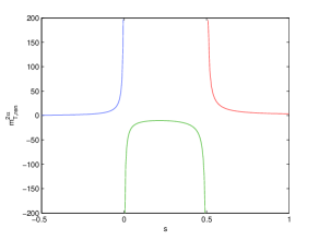
Figure 1. The dependence of the renormalized mass $m_{T,\text{ren}}^{2\alpha}$ (up to the factor (4.4)) on $s=\frac{d}{2}-\alpha$ when $p=1$ and $V=L_{1}=1$.

Figure 2. The graph and the contour lines of the renormalized mass $m_{T,\text{ren}}^{2\alpha}$ as a function of $s=\frac{d}{2}-\alpha$ and $\log L_{1}$ when $p=2$, $V=L_{1}L_{2}=1$. Due to the symmetry with respect to the interchange of $L_{1}$ and $L_{2}$, these graphs show the symmetry with respect to $\log L_{1}\mapsto-\log L_{1}$.

Figure 3. The graph and the contour lines of the renormalized mass $m_{T,\text{ren}}^{2\alpha}$ (up to the factor (4.4)) as a function of $s=\frac{d}{2}-\alpha$ and $\log k$, when $p=3$, $V=L_{1}L_{2}L_{3}=1$ and $L_{1}:L_{2}:L_{3}=k:1:1$.

Figure 4. Left: The region where $m_{T,ren}^{2\alpha}>0$ and $m_{T,\text{ren}}^{2\alpha}<0$ for $p=2$ and $V=L_{1}L_{2}=1$. Right: The region where $m_{T,\text{ren}}^{2\alpha}>0$ and $m_{T,\text{ren}}^{2\alpha}<0$ for $p=3$, $V=L_{1}L_{2}L_{3}=1$, $L_{1}:L_{2}:L_{3}=k:1:1$. Here $s=\frac{d}{2}-\alpha$.

Figure 5. The graphs of the renormalized mass $m_{T,\text{ren}}^{2\alpha}$ (up to the factor (4.4)) as a function of $s=\frac{d}{2}-\alpha$ and $\log k$ when $p=4$ and $V=L_{1}L_{2}L_{3}L_{4}=1$. For A), $L_{1}:L_{2}:L_{3}:L_{4}=k:1:1:1$. For B), $L_{1}:L_{2}:L_{3}:L_{4}=k:k:1:1$.

Figure 6. The contour lines of the graphs in Figure 5.

Figure 7. The regions where $m_{T,\text{ren}}^{2\alpha}>0$ and $m_{T,\text{ren}}^{2\alpha}<0$ when $p=4$ and $V=L_{1}L_{2}L_{3}L_{4}=1$. For A) $L_{1}:L_{2}:L_{3}:L_{4}=k:1:1:1$. For B) $L_{1}:L_{2}:L_{3}:L_{4}=k:k:1:1$. Here $s=\frac{d}{2}-\alpha$.

Figure 8. The contour lines of the renormalized mass $m_{T,\text{\text{ren}}}^{2\alpha}$ (up to the factor (4.4)) as a function of $\log k_{2}$ and $\log k_{3}$. Here $p=3$, $V=L_{1}L_{2}L_{3}=1$ and $L_{1}:L_{2}:L_{3}=1:k_{2}:k_{3}$. The values of $\frac{d}{2}-\alpha$ are $0.3,0.6,0.9,1.2,1.4$ respectively.

Figure 9. The regions where $m_{T,\text{ren}}^{2\alpha}>0$ and $m_{T,\text{ren}}^{2\alpha}<0$ for $p=3$, $V=L_{1}L_{2}L_{3}=1$, and $L_{1}:L_{2}:L_{3}=1:k_{2}:k_{3}$. Here the values of $\frac{d}{2}-\alpha$ are $0.1,0.3,0.6,0.9,1.2,1.4$.

Figure 10. The contour lines of the renormalized mass $m_{T,\text{ren}}^{2\alpha}$ (up to the factor (4.4)) as a function of $\log k_{2}$ and $\log k_{3}$, when $p=4$, $V=L_{1}L_{2}L_{3}L_{4}=1$, $L_{1}:L_{2}:L_{3}=1:k_{2}:k_{3}:k_{4}$ and $k_{4}=1$. Here the values of $\frac{d}{2}-\alpha$ are $0.1,0.4,0.8,1.2,1.6,1.9$.

Figure 11. The contour lines of the renormalized mass $m_{T,\text{ren}}^{2\alpha}$ (up to the factor (4.4)) as a function of $\log k_{2}$ and $\log k_{3}$, when $p=4$, $V=L_{1}L_{2}L_{3}L_{4}=1$, $L_{1}:L_{2}:L_{3}=1:k_{2}:k_{3}:k_{4}$ and $k_{4}=3$. Here the values of $\frac{d}{2}-\alpha$ are $0.1,0.4,0.8,1.2,1.6,1.9$.

Figure 12. The regions where $m_{T,\text{ren}}^{2\alpha}>0$ and $m_{T,\text{ren}}^{2\alpha}<0$ for $p=4$, $V=L_{1}L_{2}L_{3}L_{4}=1$, $L_{1}:L_{2}:L_{3}=1:k_{2}:k_{3}:k_{4}$ and $k_{4}=1$. The values of $\frac{d}{2}-\alpha$ are $0.1,0.4,0.8,1.2,1.6,1.9$.

Figure 13. The regions where $m_{T,\text{ren}}^{2\alpha}>0$ and $m_{T,\text{ren}}^{2\alpha}<0$ for $p=4$, $V=L_{1}L_{2}L_{3}L_{4}=1$, $L_{1}:L_{2}:L_{3}=1:k_{2}:k_{3}:k_{4}$ and $k_{4}=3$. The values of $\frac{d}{2}-\alpha$ are $0.1,0.4,0.8,1.2,1.6,1.9$.

The investigation of the sign and magnitude of the renormalized mass $m_{T,\text{ren}}^{2\alpha}$ when $p=1,2,3,4$ is carried out graphically. In Figures 1–13, we show the dependence of the renormalized mass $m_{T,\text{ren}}^{2\alpha}$ (up to the multiplicative factor (4.4)) on the compactification lengths $L_{1},\ldots,L_{p}$ and the regions where symmetry breaking mechanism appears. Using (A.3), it is found that if $\alpha\neq q/2$, then under the simultaneous scaling $L_{i}\mapsto rL_{i}$, the renormalized topologically generated mass $m_{T,\text{ren}}^{2\alpha}$ transforms according to

$$m_{T,\text{ren}}^{2\alpha}\mapsto r^{2\alpha-d}m_{T,\text{ren}}^{2\alpha}.$$

Therefore, when we study the dependence of $m_{T,\text{ren}}^{2\alpha}$ on the variables $(L_{1},\ldots,L_{p})$, we fix a degree of freedom. This can be done by letting $\mathcal{V}_{p}=\prod_{i=1}^{p}L_{i}=1$.

In Figure 1, we plot the renormalized mass $m_{T,\text{ren}}^{2\alpha}$ as a function of $\frac{d}{2}-\alpha$ when $p=1$ . The graph shows clearly that symmetry breaking appears only when $0<\frac{d}{2}-\alpha<\frac{1}{2}$. Figures 2, 3, 5 and 6 demonstrate the cases with $p=2$, $p=3$ and $p=4$. These graphs show that for suitable choices of the compactification lengths, symmetry breaking appears for all values of $\frac{d}{2}-\alpha$ lying in the range $(0,\frac{p}{2})$. In Figures 4 and 7, the unshaded regions are the regions where $m_{T,\text{ren}}^{2\alpha}<0$ and symmetry breaking exists. In all the cases considered, i.e., $p=1,2,3,4$, these regions contain the point $L_{1}=\ldots=L_{p}$ where all compactification lengths are equal, which corresponds to the lines $\log L_{1}=0$ or $\log k=0$ in the graphs.

When $p\geq 3$, after fixing one degree of freedom in the variables $(L_{1},\ldots,L_{p})$ by setting $\mathcal{V}_{p}=1$, we still have at least another two degrees of freedom. Figures 8, 10 and 11 are contour plots that show the dependence of the renormalized mass $m_{T,\text{ren}}^{2\alpha}$ on the other two degrees of freedom of the compactification lengths, for some specific values of $d-2\alpha$. In Figures 9, 12 and 13, the corresponding regions where $m_{T,\text{ren}}^{2\alpha}<0$ are shaded. From these graphs, we find that the $m_{T,\text{ren}}^{2\alpha}<0$ regions that lead to symmetry breaking are regions centered around the point $L_{1}=\ldots=L_{p}$. Moving along a ray from a point in these regions will lead to symmetry restoration. In fact, we show in [56] that the renormalized mass will become positive whenever one of the compactification lengths is large enough. The boundaries of the shaded regions in Figures 9, 12, 13 are the projections of the hypersurfaces in $(\mathbb{R}^{+})^{p}$ where $m_{T,\text{ren}}^{2\alpha}=0$ to appropriate two-dimensional planes. Note that in all the graphs, logarithm scales are used for the compactification lengths as we think that this will better illustrate the symmetry between the compactification lengths, i.e., the symmetry generated by $L_{i}\leftrightarrow L_{j}$.

From Figures 9, 12, 13, we notice that the $m_{T,\text{ren}}^{2\alpha}<0$ region (shaded) is larger when $d-2\alpha$ tends towards the boundary of the range $(0,p)$. It becomes smaller in the middle of the range $(0,p)$. We also observe a symmetry between the region for $d-2\alpha=h$ and the region for $d-2\alpha=p-h$. In fact, this is nothing but a direct consequence of the reflection formula (A.2) of the Epstein zeta function.

As mentioned above, for $p=1,2,3,4$, graphical results show that the region that lead to symmetry breaking is a region that contains the point $L_{1}=\ldots=L_{p}$. We also observed that these regions are convex and connected. We give a mathematically rigorous proof in [56] that in fact for all $p\geq 2$ and all the values of $d-2\alpha$ where symmetry breaking mechanism can exist, the region of $(L_{1},\ldots,L_{p})$ where $m_{T,\text{ren}}^{2\alpha}<0$, is a convex and therefore connected region containing the point $L_{1}=\ldots=L_{p}$, when plotted using log scale.

5. conclusion

We have studied the problem of topological mass generation for a quartic self-interacting fractional scalar Klein–Gordon field on toroidal spacetime. Our results show that the method used for ordinary scalar field, namely the zeta regularization technique, still applies with some appropriate modifications. We are able to derive the one loop effective potential for such a system for both the massless and massive case in terms of power series of $\lambda\widehat{\varphi}^{2}$ with Epstein zeta functions as coefficients. As usual in the zeta regularized method, there is a dependence of the effective potential on an arbitrary scaling length $\mu$. We proposed a scheme to renormalize the effective potential so as to get rid of the dependence on $\mu$. We have carried out a detailed derivation of the renormalization counterterms. The results of the renormalized topologically generated mass $m_{T,\text{ren}}^{2\alpha}$ are given explicitly. We note that in the massive case, $m_{T,\text{ren}}^{2\alpha}$ is always positive and therefore there is no symmetry breaking in this case. For the massless case, we show that fixing the number of compactified dimensions $p$, if $p\leq 9$, symmetry breaking appears if and only if the combination $d-2\alpha$ of spacetime dimension $d$ and fractional order $\alpha$ of Klein-Gordon field satisfies $0<d-2\alpha\leq p$. However if $p\geq 10$, symmetry breaking only exists when the value of $d-2\alpha$ lies in a proper subset of $(0,p]$. This subset becomes smaller when $p$ is increased. For all $p\geq 2$, whenever there exists symmetry breaking, symmetry restoration also appears when suitably varying the compactification lengths. Simulations are carried out to illustrate the dependence of the renormalized mass $m_{T,\text{ren}}^{2\alpha}$ on $d-2\alpha$ as well as the compactification lengths, when $p=1,2,3,4$. Graphical results show that regions that lead to symmetry breaking are always convex regions containing the point $L_{1}=\ldots=L_{p}$ where all compactification lengths are equal, agreeing with our theoretical results in [56]. It is interesting to note that we can obtain essentially the same results if instead of considering fractional scalar field of order $\alpha$ in a toroidal spacetime $T^{p}\times\mathbb{R}^{d-p}$ with integer dimension $d$, we can equivalently employ an ordinary scalar field $(\alpha=1)$ in a toroidal spacetime $T^{p}\times\mathbb{R}^{d+2-2\alpha-p}$ with fractional dimension $d+2-2\alpha$.

This paper is our first attempt to explore the fractional field theory with interactions. One possible extension of our discussion is to include local structure like spacetime curvature in addition to nontrivial global topology in our study. One expects the generalization to finite temperature case will not pose difficulty since in the Matsubara formalism, the thermal Green functions with periodic boundary condition with period given by the inverse temperature, have the same properties as the Green functions at zero temperature with the imaginary time dimension compactified to a circle of radius equals to the inverse of temperature. We can also consider the extension of our results to the fractional gauge field theory. As we mentioned in our introduction that Brownian motion plays an important role in Feynman path integrals, we would like to note that path integrals have been generalized to fractional Brownian motion [57] and fractional oscillator process [58]. Although fractional Brownian motion has found wide applications in many areas in physics and engineering, so far it has not really played a role in quantum theory yet, and no application of these ”fractional path integrals” have actually been carried out so far. In view of the fact that fractional oscillator process can be regarded as one-dimensional fractional Klein–Gordon field, with fractional Brownian motion its ”massless” limit [59, 60], it will be interesting to extend such path integrals to fractional Klein–Gordon fields and to exploit their possible uses. Finally, we would like to mention that in many applications in condensed matter physics, fractal or fractional processes have their limitations since many phenomena considered are multifractal in nature. There have already been works on multifractional Brownian motion [61, 62], multifractional Levy process [63] and multifractional oscillator process [64]. In view of the possible variable spacetime dimension, for example at the sub-Planckian distance [9], it would be interesting to consider how our results can be generalized to Klein–Gordon field with variable fractional order.

Acknowledgement  The authors would like to thank Malaysian Academy of Sciences, Ministry of Science, Technology and Innovation for funding this project under the Scientific Advancement Fund Allocation (SAGA) Ref. No P96c.

Appendix A The generalized Epstein zeta function $Z_{E,N}(s;a_{1},\ldots,a_{N};c)$

In this appendix, we summarize some facts about the generalized Epstein zeta function [65, 66] which we have used in our calculations. For details, we refer to [49, 51, 52, 53, 67, 68, 69, 70, 71, 72, 73, 74, 75, 76, 77, 78, 79] and the references therein.

A.1. Homogeneous Epstein zeta function

First consider the homogeneous Epstein zeta function $Z_{E,N}(s;a_{1},\ldots,a_{N})$. For $N\geq 1$, it is defined by the series

(A.1) $$Z_{E,N}(s;a_{1},\ldots,a_{N})=\sum_{\mathbf{k}\in\mathbb{Z}^{N}\setminus\{0\}}\left(\sum_{i=1}^{N}[a_{i}k_{i}]^{2}\right)^{-s}$$

when $\text{Re}\;\;s>\frac{N}{2}$. We extend the definition to $N=0$ by defining $Z_{E,0}(s)=0$. For $N\geq 1$, $Z_{E,N}(s;a_{1},\ldots,a_{N})$ has a meromorphic continuation to the complex plane with a simple pole at $s=N/2$, and it satisfies a functional equation (also known as reflection formula):

(A.2) $$\pi^{-s}\Gamma(s)Z_{E,N}(s;a_{1},\ldots,a_{N})=\frac{\pi^{s-\frac{N}{2}}}{\left[\prod_{j=1}^{N}a_{j}\right]}\Gamma\left(\frac{N}{2}-s\right)Z_{E,N}\left(\frac{N}{2}-s;\frac{1}{a_{1}},\ldots,\frac{1}{a_{N}}\right).$$

This formula relates the value of an Epstein zeta function at $s$ with the value of its ’dual’ at $N/2-s$. The Epstein zeta function $Z_{E,N}(s;a_{1},\ldots,a_{N})$ behaves nicely under simultaneous scaling of the parameters. Namely, for any $r\in\mathbb{R}^{+}$,

(A.3) $$Z_{E,N}\left(s;ra_{1},\ldots,ra_{N}\right)=r^{-2s}Z_{E,N}(s;a_{1},\ldots,a_{N}).$$

Together with $Z_{E,N}(0;a_{1},\ldots,a_{N})=-1$, one gets that

(A.4) $$Z_{E,N}^{\prime}\left(0;ra_{1},\ldots,ra_{N}\right)=2\log r+Z_{E,N}^{\prime}(0;a_{1},\ldots,a_{N}).$$

The function $\xi_{E,N}(s;a_{1},\ldots,a_{N})=\Gamma(s)Z_{E,N}(s;a_{1},\ldots,a_{N})$ is also a meromorphic function. For $N\geq 1$, it has simple poles at $s=0$ and $s=N/2$ with residues

(A.5) $$\text{Res}_{s=0}\Bigl{\{}\Gamma(s)Z_{E,N}(s;a_{1},\ldots,a_{N})\Bigr{\}}=-1$$

$$\text{Res}_{s=\frac{N}{2}}\Bigl{\{}\Gamma(s)Z_{E,N}(s;a_{1},\ldots,a_{N})\Bigr{\}}=\frac{\pi^{\frac{N}{2}}}{\left[\prod_{j=1}^{N}a_{j}\right]}$$

and finite parts

(A.6) $$\text{PP}_{s=0}\Bigl{\{}\Gamma(s)Z_{E,N}\left(s;a_{1},\ldots,a_{N}\right)\Bigr{\}}= Z_{E,N}^{\prime}\left(0;a_{1},\ldots,a_{N}\right)-\psi(1),$$

$$\text{PP}_{s=\frac{N}{2}}\Bigl{\{}\Gamma(s)Z_{E,N}\left(s;a_{1},\ldots,a_{N}\right)\Bigr{\}}$$

$$= \frac{\pi^{\frac{N}{2}}}{\left[\prod_{j=1}^{N}a_{j}\right]}\Biggl{[}Z_{E,N}^{\prime}\left(0;\frac{1}{a_{1}},\ldots,\frac{1}{a_{N}}\right)+2\log\pi-\psi(1)\Biggr{]}$$

respectively. Here $\psi(z)$ is the function $\Gamma^{\prime}(z)/\Gamma(z)$. Some special values of $\psi$ are $\psi(1)=-\gamma$, where $\gamma$ is the Euler constant; and for $k\geq 1$, $\psi(k+1)$ can be computed recursively by the formula

$$\psi(k+1)=\psi(k)+\frac{1}{k}.$$

One of the indispensable tools in studying the Epstein zeta function is the Chowla–Selberg formula [80, 81]. One form of the formula is

(A.7) $$\Gamma(s)Z_{E,N}(s;a_{1},\ldots,a_{N})$$

$$= 2a_{1}^{-2s}\Gamma(s)\zeta_{R}(2s)+2\sum_{j=1}^{N-1}\frac{\pi^{\frac{j}{2}}\Gamma\left(s-\frac{j}{2}\right)}{a_{j+1}^{2s-j}\prod_{l=1}^{j}a_{l}}\zeta_{R}(2s-j)+4\pi^{s}\sum_{j=1}^{N-1}\frac{1}{\prod_{l=1}^{j}a_{l}}\times$$

$$\sum_{\mathbf{k}\in{\mathbb{Z}}^{j}\setminus\{\mathbf{0}\}}\sum_{p=1}^{\infty}\frac{1}{(pa_{j+1})^{s-\frac{j}{2}}}\left(\sum_{l=1}^{j}\left[\frac{k_{l}}{a_{l}}\right]^{2}\right)^{\frac{s}{2}-\frac{j}{4}}K_{s-\frac{j}{2}}\left(2\pi pa_{j+1}\sqrt{\sum_{l=1}^{j}\left[\frac{k_{l}}{a_{l}}\right]^{2}}\right),$$

which expresses the homogeneous Epstein Zeta function as a sum of Riemann zeta function $\zeta_{R}$ plus a remainder which is a multi-dimensional series that converges rapidly. It can be used to effectively compute the homogeneous Epstein zeta function to any degree of accuracy.

A.2. Inhomogeneous Epstein zeta function

For $N\geq 1$, $a_{1},\ldots,a_{N},c>0$, the inhomogeneous Epstein zeta function $Z_{E,N}(s;a_{1},\ldots,a_{N};c)$ is defined by

$$Z_{E,N}(s;a_{1},\ldots,a_{N};c)=\sum_{\mathbf{k}\in{\mathbb{Z}}^{N}}\left(\sum_{j=1}^{N}[a_{i}k_{i}]^{2}+c^{2}\right)^{-s}$$

when $\text{Re}\,s>N/2$. When $N=0$, we define

$$Z_{E,0}(s;c)=c^{-2s}.$$

$Z_{E,N}(s;a_{1},\ldots,a_{N};c)$ has a meromorphic continuation to $\mathbb{C}$ given by

(A.8) $$Z_{E,N}(s;a_{1},\ldots,a_{N};c)=\frac{\pi^{\frac{N}{2}}}{\left[\prod_{i=1}^{N}a_{i}\right]}\frac{\Gamma\left(s-\frac{N}{2}\right)}{\Gamma(s)}c^{N-2s}$$

$$+\frac{2\pi^{s}}{\left[\prod_{i=1}^{N}a_{i}\right]\Gamma(s)}\frac{1}{c^{s-\frac{N}{2}}}\sum_{\mathbf{k}\in{\mathbb{Z}}^{N}\setminus\{\mathbf{0}\}}\left(\sum_{i=1}^{N}\left[\frac{k_{i}}{a_{i}}\right]^{2}\right)^{\frac{2s-N}{4}}K_{s-\frac{N}{2}}\left(2\pi c\sqrt{\sum_{i=1}^{N}\left[\frac{k_{i}}{a_{i}}\right]^{2}}\right).$$

The second term is an analytic function of $s$. The first term shows that $Z_{E,N}(s;a_{1},\ldots,a_{N};c)$ has simple poles at $s=\frac{N}{2}-j,j\in\mathbb{N}\cup\{0\}$ if $N$ is odd, and at $s=1,2,\ldots,\frac{N}{2}$ if $N$ is even. On the other hand, one can easily read from Eq. (A.8) that the function $\Gamma(s)Z_{E,N}(s;a_{1},\ldots,a_{N};c)$ has simple poles at $s=\frac{N}{2}-j,j\in\mathbb{N}\cup\{0\}$ with residues

(A.9) $$\text{Res}_{s=\frac{N}{2}-j}\left\{\Gamma(s)Z_{E,N}(s;a_{1},\ldots,a_{N};c)\right\}=\frac{(-1)^{j}}{j!}\frac{\pi^{\frac{N}{2}}}{\left[\prod_{i=1}^{N}a_{i}\right]}c^{2j}$$

and finite parts

(A.10) $$\text{PP}_{s=\frac{N}{2}-j}\left\{\Gamma\left(s\right)Z_{E,N}\left(s;a_{1},\ldots,a_{N};c\right)\right\}=\frac{(-1)^{j}}{j!}\frac{\pi^{\frac{N}{2}}}{\left[\prod_{i=1}^{N}a_{i}\right]}c^{2j}\left(\psi(j+1)-2\log c\right)$$

$$+\frac{2\pi^{\frac{N}{2}-j}c^{j}}{\left[\prod_{i=1}^{N}a_{i}\right]}\sum_{\mathbf{k}\in{\mathbb{Z}}^{N}\setminus\{\mathbf{0}\}}\left(\sum_{i=1}^{N}\left[\frac{k_{i}}{a_{i}}\right]^{2}\right)^{-\frac{j}{2}}K_{j}\left(2\pi c\sqrt{\sum_{i=1}^{N}\left[\frac{k_{i}}{a_{i}}\right]^{2}}\right)$$

respectively. From (A.8), (A.9) and (A.10), it can be easily deduced that

$\bullet$   If $s\notin\left\{\frac{N}{2}-j\,:\,j\in\mathbb{N}\cup\{0\}\right\}$, then

(A.11) $$\lim_{\begin{subarray}{c}a_{i}\rightarrow 0\\ 1\leq i\leq N\end{subarray}}\left[\prod_{i=1}^{N}a_{i}\right]\Bigl{\{}\Gamma(s)Z_{E,N}(s;a_{1},\ldots,a_{N};c)\Bigr{\}}=\pi^{\frac{N}{2}}\Gamma\left(s-\frac{N}{2}\right)c^{N-2s}.$$

$\bullet$   If $s=\frac{N}{2}-j$ for some $j\in\mathbb{N}\cup\{0\}$, then

(A.12) $$\lim_{\begin{subarray}{c}a_{i}\rightarrow 0\\ 1\leq i\leq N\end{subarray}}\left[\prod_{i=1}^{N}a_{i}\right]\text{Res}_{s=\frac{N}{2}-j}\Bigl{\{}\Gamma(s)Z_{E,N}(s;a_{1},\ldots,a_{N};c)\Bigr{\}}=\frac{(-1)^{j}}{j!}\pi^{\frac{N}{2}}c^{2j}.$$

(A.13) $$\lim_{\begin{subarray}{c}a_{i}\rightarrow 0\\ 1\leq i\leq N\end{subarray}}\left[\prod_{i=1}^{N}a_{i}\right]\text{PP}_{s=\frac{N}{2}-j}\Bigl{\{}\Gamma(s)Z_{E,N}(s;a_{1},\ldots,a_{N};c)\Bigr{\}}=\frac{(-1)^{j}}{j!}\pi^{\frac{N}{2}}c^{2j}\left(\psi(j+1)-2\log c\right).$$

Appendix B Independence of $V_{\text{eff}}^{(\text{ren})}$ on $\mu$

Here we give a sketch of the proof that the renormalized effective potential $V_{\text{eff}}^{(\text{ren})}(\widehat{\varphi})$ is independent of $\mu$. From the definition of the renormalized effective potential (3.1) and the formula (3.4) that determines the counterterms, we get

$$V_{\text{eff}}^{(\text{ren})}(\widehat{\varphi})=\frac{1}{2}m^{2\alpha}\widehat{\varphi}^{2}+\frac{1}{4!}\lambda\widehat{\varphi}^{4}+V_{Q}+\Lambda\Pi^{-1}T,$$

where

$$\Lambda=\begin{pmatrix}1&\frac{\widehat{\varphi}^{2}}{2!}&\frac{\widehat{\varphi}^{4}}{4!}&\ldots&\frac{\widehat{\varphi}^{2d_{\alpha}}}{(2d_{\alpha})!}\end{pmatrix},\hskip 28.45274ptT=\begin{pmatrix}T_{0}\\ T_{1}\\ \vdots\\ T_{d_{\alpha}}\end{pmatrix}.$$

The terms containing $\log\mu^{2}$ can be extracted from $V_{Q}$ (eq. (2.26) and (2.27)) and $T_{j}$ (eq. (3.5) and (3.11)), with result given by

(B.1) $$\Lambda S^{\mu}+\Lambda\Pi^{-1}T^{\mu},$$

where

$\bullet$  in the massive case,

$$S^{\mu}_{k}=\frac{m^{d}}{2^{d+1}\pi^{\frac{d}{2}}}\frac{(-1)^{k}(2k)!}{\Gamma(\alpha k+1)}\left(\frac{\lambda}{2m^{2\alpha}}\right)^{k}\frac{(-1)^{\frac{d}{2}-\alpha k}}{\left(\frac{d}{2}-\alpha k\right)!}\chi_{k;\alpha;d},$$

with

$$\chi_{k;\alpha;d}=\begin{cases}1,\hskip 28.45274pt&\text{if}\;\;k\in\mathcal{H}_{\alpha;d,0},\\ 0,&\text{otherwise},\end{cases}$$

and

$$T^{\mu}_{j}= \frac{(-1)^{j+1}\lambda^{j}m^{d-2\alpha j}}{2^{d+j+1}\pi^{\frac{d}{2}}}\sum_{k\in\mathcal{H}_{\alpha;d,j}}\frac{(-1)^{k+\frac{d}{2}-\alpha(k+j)}[2(k+j)]!}{[2k]!\left[\frac{d}{2}-\alpha(k+j)\right]!\Gamma(\alpha(k+j)+1)}\left(\frac{\lambda\widehat{\varphi}^{2}_{j}}{2m^{2\alpha}}\right)^{k}.$$

$\bullet$   in the massless case,

$$S^{\mu}_{k}=\frac{(-1)^{\frac{d}{2\alpha}}\delta_{k,d_{\alpha}}\omega_{\alpha;d}}{2^{d+1}\pi^{\frac{d}{2}}\Gamma\left(\frac{d+2}{2}\right)}(2k)!\left(\frac{\lambda}{2}\right)^{k},$$

and

$$T_{j}^{\mu}=-\frac{\omega_{\alpha;d}}{2^{d+1}\pi^{\frac{d}{2}}}\frac{(-1)^{\frac{d}{2\alpha}}}{\Gamma\left(\frac{d}{2}+1\right)}\frac{\lambda^{j}}{2^{j}}\left(\frac{\lambda\widehat{\varphi}_{j}^{2}}{2}\right)^{\frac{d}{2\alpha}-j}\frac{\left(\frac{d}{\alpha}\right)!}{\left(\frac{d}{\alpha}-2j\right)!}.$$

In both cases, it is easy to verify that $\Pi S^{\mu}=-T^{\mu}$, which shows that the term (B.1) is identically zero and therefore $V_{\text{eff}}^{(\text{ren})}(\widehat{\varphi})$ does not depend on $\log\mu^{2}$.

References

- [1] B. B. Mandelbrot, The fractal geometry of nature, (W.H. Freeman, New York, 1983).
- [2] R.P.Feynman and A.R. Hibbs, Quantum mechanics and path integrals, (McGraw-Hill, New York, 1965).
- [3] L.F. Abbot and M.B. Wise, Dimension of a quantum–mechanical path, Am. J. Phys. 49, 37–39 (1981).
- [4] E. Nelson, Derivation of Schrödinger equation from Newtonian mechanics, Phys. Rev. 150, 1079–1085 (1966).
- [5] E. Nelson, Quantum fluctuations, (Princeton University Press, N. J., 1985).
- [6] H. Kroger, Fractal geometry in quantum mechanics, field theory and spin systems, Phys. Rep. 323, 81–181, 2000.
- [7] H. J. Rothe, Lattice gauge theories: An introduction, 3rd edition (World Scientific, Singapore, 2005).
- [8] B. J. Durhuus, J. Ambjorn, Quantum geometry: A statistical field theory approach, (Cambridge University, Cambridge, 1997).
- [9] , O. Lauscher and M. Reuter, Fractal spacetime structure in asymptotically safe gravity, Preprint arXiv:hep-th/0508202, 2005.
- [10] K. S. Miller and B. Ross, An introduction to the fractional calculus and fractional differential equations, (John Wiley and Sons, New York, 1993).
- [11] S. Samko, A.A. Kilbas and D.I. Maritchev, Integrals and derivatives of the fractional order and some of their applications, (Gordon and Breach, Armsterdam, 1993).
- [12] I. Podlubny, Fractional differential equations, (Academic Press, New York, 1999).
- [13] A. A. Kilbas, H. M. Srivastava and J. J. Trujillo, Theory and applications of fractional differential equations, (Elsevier, Amsterdam, 2006).
- [14] R. Hilfer ed., Applications of fractional calculus in physics, (World Scientific, Singapore, 2000).
- [15] B. J. West, M. Bologna and P. Grigolini, Physics of fractal operators, (Springer- Verlag, New York, 2003).
- [16] R. Metzler and J. Klafter, The restaurant at the end of the random walk: Recent developments in the description of anomalous transport by fractional dynamics, J Phys. A 37, R161-R208 (2004).
- [17] L. M. Zelenyi and A. V. Milovanov, Fractal topology and strange kinetics: from percolation theory to problems in cosmic electrodynamics, Phys. Uspekhi 47, 749–788 (2004).
- [18] G. M. Zaslavsky, Hamiltonian chaos and fractional dynamics, (Oxford: Oxford University, 2005).
- [19] Y. Hu and G. Kallianpur, Schr dinger equation with fractional Laplacian, Appl. Math. Optim. 42, 281–290 (2000).
- [20] N. Laskin, Fractals and quantum mechanics, Chaos, 10, 780–790 (2000).
- [21] N. Laskin, Fractional Schr dinger equation, Phys. Rev. E 66, 056108, (2002).
- [22] M. Naber, Time fractional Schr dinger equation, J. Math. Phys. 45, 3339–3352 (2004).
- [23] X. Guo and M. Xu, Some applications of fractional Schr dinger equation, J. Math. Phys. 47, 082104 (2006).
- [24] S. Wong and M. Xu, Generalized fractional Schr dinger equation with space-time fractional derivatives, J. Math. Phys. 48, 043502 (2007).
- [25] J. Dong and M. Xu, Some solutions to the space fractional Schr dinger equation using momentum representation method, J. Math. Phys. 48, 072105 (2007).
- [26] D. Baleanu and S.I. Muslih, About fractional supersymmetric quantum mechanics, Czech. J. Phys. 55, 1063–1066 (2005).
- [27] C. G. Bollini and J. J. Giambiagi, Arbitrary powers of D’Alembertian and the Huygens’ principle, J. Math. Phys. 34, 610–621 (1993).
- [28] C. Lammerzahl, The pseudodifferential operator square root of the Klein–Gordon equation, J. Math. Phys. 34, 3918–3932 (1993).
- [29] M. S. Plyushchay and M. R. de Traubenberg, Cubic root of Klein–Gordon equation, Phys. Lett. B 477, 276–284 (2000).
- [30] Kh. Namsrai and H. V. von Geramb, Square–root operator quantization and nonlocality: a review, Int. J. Theor. Phys. 40, 1929–2010 (2001).
- [31] A. Raspini, Simple solution of fractional Dirac equation of order 2/3, Physica Scripta 64, 20–22 (2001).
- [32] P. Zavada, Relativistic wave equations with fractional derivatives and pseudo-differential operators, J. Appl. Math. 2, 163–197 (2002).
- [33] R. L. P. G. do Amaral and E. C. Marino, Canonical quantization of theories containing fractional powers of the d’Alembertian operator, J. Phys. A: Math. Gen. 25, 5183–5200 (1992).
- [34] D. G. Barci, L. E. Oxman, and M. Rocca, Canonical quantization of non-local field equations, Int. J. Mod. Phys. A 11, 2111–2126 (1996).
- [35] S. C. Lim and S. V. Muniandy, Stochastic quantization of nonlocal fields, Phys. Lett. A 324, 396–405 (2004).
- [36] S. Albeverio H. Gottschalk and J.-L Wu, Convoluted generalized white noise, Schwinger functions and their analytic continuation to Wightman functions, Rev. Math. Phys. 8, 763–817 (1996).
- [37] M. Grothaus and L. Streit, Construction of relativistic quantum fields in the framework of white noise analysis, J. Math. Phys. 40, 5387–5405 (1999).
- [38] S.C. Lim, Fractional derivative quantum fields at positive temperature, Physica A 363, 269–281 (2006).
- [39] C. H. Eab, S. C. Lim and L. P. Teo, Finite temperature Casimir effect for a massless fractional Klein-Gordon field with fractional Neumann conditions, J. Math. Phys. 48, 082301 (2007).
- [40] M. E. Peskin and D. V. Schroeder, An introduction to quantum field theory, (Addison-Wesley, Reading, 1995).
- [41] E. W. Kolb and M. S. Turner, The early universe, (Addison-Wesley, Reading, 1990).
- [42] J.Zinn-Justin, Quantum field theory and critical phenomena, (Clarendon Press, Oxford, 4th Edition, 2002).
- [43] T. Dauxois and M. Peyrard, Physics of solitons, (Cambridge University Press, Cambridge, 2006).
- [44] L. H. Ford and T. Yoshimura, Mass generation by self–interaction in non-Minkowskian spacetimes, Phys. Lett. A 70, 89–91 (1979).
- [45] D. J. Toms, Symmetry breaking and mass generation by space-time topology, Phys. Rev. D 21, 2805–2817 (1980).
- [46] G. Denardo and E. Spallucci, Dynamical mass generation in , Nucl. Phys. B 169, 514–526 (1980).
- [47] A. Actor, Topological generation of gauge field mass by toroidal spacetime, Class. Quantum Grav. 7, 663–683 (1980).
- [48] K. Kirsten, Topological gauge field mass generation by toroidal spacetime, J. Phys. A: Math. Gen. 26, 2421–2435 (1993).
- [49] E. Elizalde and K. Kirsten, Topological symmetry breaking in self-interacting theories on toroidal space-time, J. Math. Phys. 35, 1260–1273 (1994).
- [50] S. W. Hawking, Zeta function regularization of path integrals in curved space time, Comm. Math. Phys. 55, 139–170 (1977).
- [51] E. Elizalde, S. D. Odintsov, A. Romeo, A. A. Bytsenko, and S. Zerbini, Zeta regularization techniques with applications, (World Scientific Publishing Co. Inc., River Edge, NJ, 1994).
- [52] Emilio Elizalde, Ten physical applications of spectral zeta functions, (Springer-Verlag, Berlin, 1995).
- [53] K. Kirsten, Spectral functions in mathematics and physics, (Chapman & Hall/ CRC, Boca Raton, FL, 2002).
- [54] E. Elizalde, K. Kirsten and S. Zerbini, Applications of the Mellin–Barnes integral representation, J. Phys. A: Math. Gen. 28 (1995), 617–629.
- [55] S. C. Lim and L. P. Teo, Finite temperature Casimir energy in closed rectangular cavities: a rigorous derivation based on zeta function technique, J. Phys. A: Math. Theor. 40 (2007), 11645-11674.
- [56] S. C. Lim and L. P. Teo, On the minima and convexity of Epstein Zeta function, in preparation.
- [57] K. L. Sebastian, Path integral representation for fractional Brownian motion, J. Phys. A: Math. Gen. 28 4305 (1995).
- [58] C. H. Eab and S. C. Lim, Path integral representation of fractional harmonic oscillator, Physica A 371, 303–316 (2006).
- [59] S. C. Lim, M. Li and L. P.Teo, Locally self-similar fractional oscillator processes, Fluct. Noise Lett. 7, L169–L179 (2007).
- [60] S. C. Lim and C. H. Eab, Riemann–Liouville and Weyl fractional oscillator processes, Phys. Lett. A 335, 87–93 (2006).
- [61] R. Peltier and J. Levy Vehel, Multifractional Brownian motion: Definition and preliminary results, INRIA Report 2645 (1995).
- [62] A. Benassi, S. Jaffard and D. Roux, Elliptic Gaussian random processes, Rev. Mat. Ibroamericana 13, 19–90 (1997).
- [63] C. Lacaux, Real harmonizable multifractional Levy motions, Ann. Inst. Henri Poincare-Probab. Stat. 40, 259–277 (2004).
- [64] S. C. Lim and L. P. Teo, Weyl and Riemann–Liouville multifractional Ornstein–Uhlenbeck processes, J. Phys. A: Theo. Gen. 40, 6035–6060 (2007).
- [65] P. Epstein, Zur Theorie allgemeiner Zetafunktionen, Math. Ann. 56, 615–644 (1903).
- [66] P. Epstein, Zur Theorie allgemeiner Zetafunktionen II, Math. Ann. 65, 205–216 (1907).
- [67] J. Jorgenson and S. Lang, Complex analytic properties of regularized products, Lect. Notes Math. 1564, (Springer-Verlag, 1993).
- [68] P. Sarnak, Determinants of Laplacians, Comm. Math. Phys. 110, 113–120 (1987).
- [69] M. Spreafico, Zeta functions, special functions and the Lerch formula, Proc. Royal Soc. Ed. 136A, 865–889 (2006).
- [70] I. Vardi, Determinants of Laplacians and multiple Gamma functions, SIAM J. Math. Anal. 19, 493-507 (1988).
- [71] A. Voros, Spectral functions, special functions and the Selberg zeta function, Comm. Math. Phys. 110, 439-465 (1987).
- [72] E. Elizalde and A. Romeo, Regularization of general multidimensional Epstein zeta-functions, Rev. Math. Phys. 1 (1989), no. 1, 113–128.
- [73] K. Kirsten, Inhomogeneous multidimensional Epstein zeta functions, J. Math. Phys. 32, no. 11, 3008–3014 (1991).
- [74] K. Kirsten, Generalized multidimensional Epstein zeta functions, J. Math. Phys. 35 (1994), no. 1, 459–470.
- [75] E. Elizalde, An extension of the Chowla-Selberg formula useful in quantizing with the Wheeler-DeWitt equation, J. Phys. A 27, no. 11, 3775–3785 (1994).
- [76] E. Elizalde, Extension of the Chowla-Selberg formula and applications, Group theoretical methods in physics (Toyonaka, 1994), (World Sci. Publ., River Edge, NJ, 1995), pp. 191–194.
- [77] E. Elizalde, Multidimensional extension of the generalized Chowla-Selberg formula, Comm. Math. Phys. 198, no. 1, 83–95 (1998).
- [78] E. Elizalde, Zeta functions: formulas and applications, J. Comput. Appl. Math. 118, no. 1-2, 125–142, Higher transcendental functions and their applications (2000).
- [79] E. Elizalde, Explicit zeta functions for bosonic and fermionic fields on a non-commutative toroidal spacetime, J. Phys. A 34, no. 14, 3025–3035 (2001).
- [80] S. Chowla and A. Selberg, On Epstein’s zeta function. I, Proc. Nat. Acad. Sci. U. S. A. 35, 371–374 (1949).
- [81] A. Selberg and S. Chowla, On Epstein’s zeta-function, J. Reine Angew. Math. 227, 86–110 (1967).