Chapter 1 Neutrino Interactions

Kevin McFarland
University of Rochester, Rochester, NY, USA 14627

1 Introduction and Motivations

The study of neutrino interaction physics played an important role in establishing the validity of the theory of weak interactions and electroweak unification. Today, however, the study of interactions of neutrinos takes a secondary role to studies of the properties of neutrinos, such as masses and mixings. This brief introduction describes the historical role that the understanding of neutrino interactions has played in neutrino physics and what we need to understand about neutrino interactions to proceed in future experiments aimed at learning more about neutrinos.

The original application of neutrino interactions was the discovery of the neutrino itself. For most physicists today, who came of age professionally well after the first observation of neutrinos, it takes a bit of thought to understand the perspective of the experimenters seeking to discover the neutrino. A close analogy today might be the search for interactions of weakly interacting massive (WIMP) dark matter particles. In order to sensibly design an experiment to search for a new particle and to interpret the results, an experimenter needs guidance about the probable type and rate of interactions to be observed. For the case of WIMP dark matter, information about the strength of interactions comes from the standard cosmological model which relates modern day abundance of dark matter to production and annihilation cross sections.

In the case of neutrinos in the early 1950s, the guiding principle was the Fermi “four fermion” theory of the weak interaction (Fermi 1934). This theory introduced a four-fermion vertex connecting a neutron $n$, a proton $p$, an electron $e^{-}$ and an anti-neutrino, $\nu$ or $\bar{\nu}$ to explain neutron decay, $n\to pe^{-}\bar{\nu}$ in terms of a single unknown coupling constant, $G_{F}$. Because that single constant governed the strength of all weak interactions among these particles, the Fermi theory led to definite prediction for neutrino interactions involving these particles. The prediction for the cross section of $\bar{\nu}p\to e^{+}n$ was first derived by Bethe and Peierls shortly after the Fermi theory was published (Bethe and Peierls 1934). For neutrinos with energies of a few MeV from a reactor, a typical cross section in this theory was predicted to be $\sigma_{\bar{\nu}p}\sim 5\times 10^{-44}$ cm². Interestingly, this prediction for reactor neutrino cross sections is still accurate today, up to a factor of two required to account for the then unknown phenomenon of maximal parity violation in the weak interaction! This small cross section is, as we all recognize today, the primary challenge in performing experiments with neutrinos. By contrast, the cross section for the corresponding electromagnetic process with a photon $\gamma$ at similar energies is $\sigma_{\gamma p}\sim 10^{-25}$ cm². The tiny neutrino cross section means that the mean free path of reactor neutrinos with energies of a few MeV in steel is approximately ten light years.

With these predictions in place, the stage was set for the two critical measurements establishing the existence and nature of the neutrinos from nuclear reactors: the Davis et al null measurement of the reaction $\bar{\nu}~{}+~{}^{37}Cl~{}\to~{}^{37}Ar~{}+~{}X$ and Reines and Cowan’s observation of $\bar{\nu}p\to e^{+}n$ in 1955-56. In modern language, the latter measurement establishes the existence of the neutrino and validates the universality of the Fermi theory and the former non-measurement shows that the neutrino and anti-neutrino carry an opposite conserved lepton number which forbids $\bar{\nu}n\to e^{-}p$ (Reines 1996).

1.1 A Cautionary Tale: Discovery of the Weak Neutrino Current

A more sobering story involving knowledge of neutrino cross sections involves the discovery of the weak neutral current in neutrino interactions. No textbook would be complete without the requisite picture of the famous single electron event in the Gargamelle bubble chamber, attributed to $\bar{\nu}_{e}e^{-}\to\bar{\nu}_{e}e^{-}$. While this event is a wonderful illustration of a weak neutrino process, it was not the discovery channel. As we will see, the cross section for this reaction is exceedingly small, and concerns about backgrounds and the lack of corroborating information in such a reaction make it a difficult channel in which to claim a discovery. The discovery measurement for the weak neutral current involves processes where neutrinos scatter off of the nuclei in the target allowing the experimenters to measure a quantity such as

$$R^{\nu}=\frac{\sigma(\nu_{\mu}N\to\nu_{\mu}X)}{\sigma(\nu_{\mu}N\to\mu^{-}X)}$$ (1)

or its analog with an anti-neutrino beam. Figure 1 shows these two measurements compared with the prediction of the electroweak standard model as a function of its single parameter not constrained by low energy data, $\sin^{2}\theta_{W}$, which is the weak mixing angle or Weinberg angle.

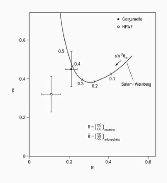
Figure 1: Measurement of $R^{\bar{\nu}}$ vs. $R^{\nu}$ from the Gargamelle and HWPF collaborations compared with the prediction of the electroweak standard model.

This major triumph for the standard model of electroweak unification was sadly complicated by an involved saga which ultimately boiled down to uncertainties in translating observed events to the measurement of $R^{\nu}$. Experimentally, the measurement consists of identifying events as either containing or not containing of final state muon and using this distinguishing feature to separate charged and neutral current interactions. Very low energy muons are difficult to separate from other particles, primarily charged mesons, produced in inelastic scattering from nuclei, and so these events constitute a background to the neutral current sample. Equally problematic for this measurement are neutral current events which produce charged hadrons in the final state that are confused with energetic muons. Without a good model for the production of these charged mesons or a good understanding of the probability of confusing charged mesons with muons in the detector, the experimental problem of isolating sufficiently clean samples with high statistics hobbled efforts to produce a convincing observations by both of the competing collaborations, Gargamelle at CERN and HWPF at Fermilab (Galison 1983). It is notable that this important discovery was never honored with a Nobel prize, despite its critical role in validating the electroweak theory.

1.2 Cross Section Knowledge and Next Generation Oscillation Experiments

The current and next generation of accelerator neutrino oscillation experiments are again facing limitations arising from knowledge of neutrino cross sections. The physics roadmap of precisely measuring the “atmospheric” oscillation parameters, measuring $\theta_{13}$, determining the neutrino mass hierarchy and measuring the CP violating phase, $\delta$, has driven an experimental program to be realized in several steps. Currently this program is the measurement of $\nu_{\mu}\to\nu_{\mu}$ transition probabilities in wide band beams with baseline $L$ and mean energies $E$ near $L/E\sim 400$ km/GeV (K2K and MINOS), and the measurement of $\nu_{\mu}\to\nu_{\tau}$ near $\tau$ production threshold (OPERA). In the near future, it includes narrowband (off-axis) beam experiments again near $L/E\sim 400$ km/GeV to precisely measure $\nu_{\mu}\to\nu_{e}$ transitions in neutrino and anti-neutrino beams (T2K and NOvA). Most likely, completion of this program will require a new generation of experiments to study these transitions at the second oscillation maximum as well, $L/E\sim 1200$ km/GeV, either in narrow band beams (T2KK) or wideband beams (discussed in FNAL to DUSEL proposals). Practical considerations limit the range of possible baselines to $L\stackrel{{\scriptstyle<}}{{\sim}}2000$ km because of available sites and achievable event rates and $E\stackrel{{\scriptstyle>}}{{\sim}}0.5$ GeV because of the roughly quadratic drop in the signal cross section and because of significant nuclear effects with neutrinos energies below this limit. This implies that the neutrinos to be studied will have $0.5<E_{\nu}<5$ GeV. As we will see, this region is at the threshold for inelastic interactions on nucleons, which is a particularly difficult energy region to model and is lacking in data to contribute to understanding the relevant effects governing the details of cross sections.

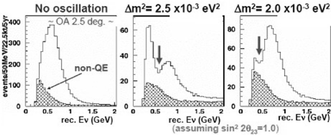
Figure 2: The expected far detector $\nu_{\mu}$ candidate spectrum in the T2K experiment for $\theta_{23}=\pi/4$. The hatched area in each plot shows expected backgrounds.

Knowledge of cross sections impacts a $\nu_{\mu}\to\nu_{\mu}$ disappearance measurement in this energy regime because, regardless of experimental techniques, the details of the final state will impact the separation of signal from background and the measurement of neutrino energy in a given event. Figure 2 illustrates the effect of backgrounds on the measurement of the maximum oscillation probability on the T2K experiment. If the background to the signal, in this case primarily from inelastic charged-current events, cannot be accurately estimated, then it becomes difficult to measure the depth of the oscillation “dip” which is used to measure $\theta_{23}$. In a broadband beam like that of the MINOS experiment where the neutrinos at the energy of maximal oscillation have an energy near $2$ GeV, the differences in energy response between baryons, charged pions and neutral pions in the final state lead to a significant uncertainty in reconstructed energy. This uncertainty in turn impacts the measurement of the energy of the oscillation “dip” which determines $\delta m^{2}_{23}$.

Figure 3: Knowledge of single $\pi^{0}$ neutrino production cross sections as a function of energy before K2K or MiniBooNE results (Zeller 2003).

Figure 4: The anti-neutrino vs. neutrino $\nu_{\mu}\to\nu_{e}$ transition probability in percent a baseline of $700$ km at different energies for different mass hierarchies and values of the CP violating phase $\delta$ (Minakata and Nunokata 2001).

Because the $\nu_{\mu}\to\nu_{e}$ oscillation probability is so low, the major impact on these appearance experiments, such as T2K and NOvA, is expected to be from backgrounds to electron appearance. The major such background is the production of neutral pions which decay into photons that shower and mimic electrons, either because of a merging or loss of $\gamma$ rings in a Cerenkov detector or because of the merging or loss of one $\gamma$ in a calorimetric detector. Unfortunately, this background is poorly constrained by existing data (Figure 3). The challenge becomes apparent when looking at the precision needed for the physics goals of these experiments. Ultimately, as illustrated in Figure 4, the transition probabilities will need to be measured with sub-percent precision to measure the effect of CP violation in neutrinos. This places strict requirements on the understanding of $\nu_{e}$ backgrounds in both neutrino and anti-neutrino beams.

This interest in neutrino interactions in the $0.5$ to $5$ GeV energy region has led to the proposal and construction of a number of dedicated neutrino cross section experiments designed to make these measurements. The K2K experiment recently built a near detector, “SciBar”, designed for such measurements which is currently running as “SciBooNE” in the Fermilab Booster neutrino beam. The MINERvA experiment is currently under construction for future operation in the Fermilab NuMI beamline.

2 Pointlike Interactions

For a pedagogical explanation of neutrino cross section phenomenology, it is helpful to start with the scattering of neutrinos from effectively massless pointlike fermions, such as neutrino-electron scattering. Although this interaction is of limited practical interest for accelerator oscillation experiments, the calculation of pointlike scattering will serve multiple purposes as we begin to explore more complicated cross section phenomenology. First, in the high energy limit of neutrino-nucleon scattering, a good approximation to deep inelastic scattering is to consider the scattering of neutrinos on point-like quark constituents of the nucleus. Second, the study of scattering from pointlike particles will make a good point of departure from which to study effects such as initial and final state masses and the effect of structure in a target fermion. Therefore, please suspend skepticism of the usefulness of this particular exercise, and let us begin to consider neutrino scattering on electrons.

The style of the lectures was to present examples illustrating the phenomena of neutrino interactions. Accordingly, what follows below uses heuristic arguments and does not follow a style of rigorous proof. To paraphrase the humorist Michael Feldman, readers who are sticklers for the whole truth should write their own lectures.

2.1 Weak Interactions and Neutrinos

The modern view of the weak interaction is not the four fermion interaction of Fermi’s theory, but rather an interaction mediated by the exchange of massive $W$ and $Z$ bosons. In the low momentum limit, where the mediating boson is far off shell, the weak interaction Hamiltonian governing the process $\nu f\to\ell/\nu+f^{\prime}$ is

$${\cal H}_{weak}=\frac{4G_{F}}{\sqrt{2}}\left[\bar{\ell}/\bar{\nu}\gamma_{\mu}\frac{(1-\gamma_{5})}{2}\nu\right]\left[\bar{f^{\prime}}\gamma^{\mu}\left(g_{L}\frac{1-\gamma_{5}}{2}+g_{R}\frac{1+\gamma_{5}}{2}\right)f\right]+{\rm\textstyle h.c.}$$ (2)

where $f$, $f^{\prime}$, $l$ and $\nu$ stand for an initial and final state fermion, lepton and neutrino, respectively, $g_{L}$ and $g_{R}$ are the weak neutral-current chiral couplings, $\gamma_{\mu}$ are the standard Dirac matrices and $\gamma_{5}\equiv i\gamma_{0}\gamma_{1}\gamma_{2}\gamma_{3}$. Note that, like the Fermi theory, this form makes reference to a single coupling constant, $G_{F}$, to which we shall return later. It does include an important component not recognized in the Fermi theory, namely parity non-conservation. The factor $(1-\gamma_{5})/2$ is a projection operator onto left-handed states for fermions and right-handed states for anti-fermions.

Table 1: Weak neutral-current couplings $g_{L}$ and $g_{R}$.

$Z$ coupling	$g_{L}$	$g_{R}$
$\nu$	$1/2$	$0$
$e$,$\mu$,$\tau$	$-1/2+\sin^{2}\theta_{W}$	$\sin^{2}\theta_{W}$
$u$,$c$,$t$	$1/2-(2/3)\sin^{2}\theta_{W}$	$-(2/3)\sin^{2}\theta_{W}$
$d$,$s$,$b$	$-1/2+(1/3)\sin^{2}\theta_{W}$	$(1/3)\sin^{2}\theta_{W}$

The Hamiltonian above also has provision for a neutral-current interaction, mediated by the $Z$, in which the neutrino remains a neutrino, and a charged-current interaction, mediated by the $W$ in which the neutrino becomes a charged lepton. A neutrino, weak or flavor, eigenstate, $\nu_{e}$, $\nu_{\mu}$ or $\nu_{\tau}$, is associated with the production of a charged lepton of the same generation in the charged-current weak interaction. The weak interaction is maximally parity-violating in the charged-current interaction, selecting only left-handed fermions, and therefore the right handed charged-current couplings are zero. However, in the case of the neutral weak interaction, these couplings are given in terms of the electromagnetic and weak couplings by the electroweak unification theory and their values for each species of fermion are given in Table 1. Note the right-handed neutrino has no weak couplings, neither in the neutral nor the charged current, which makes it unique among the fermions.

The rigorous definition of this “handedness”, or chirality, is equivalent to the definition of the left-handed (right-handed) projection operator, $(1\mp\gamma_{5})/2$. If a particle is massless, this chirality is equivalent to its helicity, i.e. the projection of its spin $\sigma$ along the direction of the particle, $\sigma\cdot\hat{p}$. The Hamiltonian above indicates that neutrinos produced or participating in weak interactions will be entirely left-handed. Since neutrinos do have mass, $m_{\nu}$, this implies that while the neutrino will primarily be negative helicity, there will be a small positive helicity component, frame-dependent, and proportional to $m_{\nu}/E_{\nu}$ where $E_{\nu}$ is the neutrino energy. For most practical purposes, this positive helicity component can be entirely neglected.

Figure 5: Similarity of the strength of weak and electromagnetic interactions at high momentum transfer as illustrated by measurements of neutral and charged-current $ep$ scattering measured by the ZEUS experiment at HERA.

The final aspect of this form of the weak interaction to be explained is the Fermi constant itself, $G_{F}\approx 1.166\times 10^{-5}$ GeV^-2. The dimensions and size of the Fermi constant, which make the weak interaction “weak” at low energies, have their origin in the propagator associated with the exchange of the $W$ boson. For a two body massless weak scattering process,

$$\frac{d\sigma}{dq^{2}}\propto\frac{1}{(q^{2}-M_{W}^{2})^{2}},$$ (3)

where $M_{W}$ and $q$ are the mass of and the four-momentum carried by the $W$ boson. For $|q^{2}|\ll M_{W}^{2}$, this propagator term gives a factor of $M_{W}^{-4}$. In the case of the electromagnetic interaction, this same term becomes $q^{-4}$ since the mass of the exchanged boson, the photon, is zero. Figure 5 shows cross sections of the neutral current process, $e^{-}p\to e^{-}p$, which has contributions from both $\gamma$ and $Z^{0}$ exchange, and the charged current process, $e^{-}p\to\nu X$, which is purely weak. In these processes, $q^{2}<0$, and we usually write $Q^{2}=-q^{2}$ by convention. We see that when $Q^{2}<M_{W}^{2}$, the neutral current cross section is rapidly falling with $Q^{2}$, while the charged-current cross section is roughly constant. However, beginning at $Q^{2}\sim M_{W}^{2}$, both cross sections are roughly comparable and falling steeply with $Q^{2}$. In the electroweak theory, $G_{F}$ can be expressed in terms of $M_{W}$ and an overall weak coupling constant, $g_{W}$, as

$$G_{F}=\frac{\sqrt{2}}{8}\left(\frac{g_{W}}{M_{W}}\right)^{2};$$ (4)

therefore, $g_{W}$ is a coupling of ${\cal O}(1)$ and roughly the same size as the electromagnetic coupling constant in this unified theory of the two interactions.

2.2 Neutrino Electron Scattering

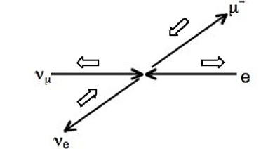
Figure 6: Helicity in the massless limit of neutrino-electron scattering.

With this background, we are ready to calculate a neutrino-electron scattering cross section. For pedagogical simplicity, first consider $\nu_{\mu}e^{-}\to\mu^{-}\nu_{e}$ at sufficiently high energies so that we may neglect all masses in the problem, including the mass of the final state muon, but not at such high energies that we need worry about the effect of $Q^{2}$ on the propagator $1/(Q^{2}+M_{W}^{2})^{2}$. In this limit, chirality is equivalent to helicity. In the center-of-mass frame we can easily see that the two left-handed and negative helicity particles in the final state have a total spin along the interaction axis of $J_{z}=0$ (Figure 6), and therefore there is no preferred center-of-mass scattering angle. Thus,

$$\sigma=\int_{0}^{Q^{2}_{MAX}}dQ^{2}\frac{d\sigma}{dQ^{2}}\propto\int_{0}^{Q^{2}_{MAX}}dQ^{2}\frac{1}{(Q^{2}+M_{W}^{2})^{2}}=\frac{Q^{2}_{MAX}}{M_{W}^{4}}.$$ (5)

That’s it! To complete the evaluation of the cross section, we need only find the constant of proportionality, which turns out to be $g_{W}^{4}/32\pi=M_{W}^{4}\times G_{F}^{2}/\pi$, and the maximum $Q^{2}$ that can be exchanged. Here $Q^{2}$, the negative of the square of the four-momentum carried by the $W$ boson, is $-(\underline{e}-\underline{\nu}_{e})^{2}$, where the underlined terms represent four-vectors. It is simple to show that, in terms of $E^{*}_{\nu}$ and $\theta^{*}$ the center-of-mass energy and scattering angle, $Q^{2}=2{E^{*}_{\nu}}^{2}(1-\cos\theta^{*})$. This means that $Q^{2}$ ranges between $0$ and $4{E^{*}_{\nu}}^{2}=s$ where $\sqrt{s}$ is the total available center-of-mass energy. The cross section is therefore

$$\sigma=\frac{G_{F}^{2}s}{\pi}.$$ (6)

Numerically, this turns out to be $\sigma=17.2\times 10^{-42}$ cm${}^{2}\times E_{\nu}$/GeV. The proportionality to the neutrino energy in the lab frame comes about computationally because, if the target electron is at rest, $s=m_{e}^{2}+2m_{e}E_{\nu}$ and the $m_{e}^{2}$ term can be neglected for neutrino beam energies of interest. More fundamentally, this proportionality to energy is a generic feature of pointlike neutrino scattering at $Q^{2}$ below $M_{W}^{2}$ squared, since $d\sigma/dQ^{2}$ is constant.

We now consider another process, this time the neutral current elastic scattering $\nu_{\mu}e^{-}\to\nu_{\mu}e^{-}$. How is this process different from our previous example under the same energy approximations? First, the process is a neutral current one, and therefore, as can be seen in Table 1, the interaction couples to both the left-handed and right-handed electron. In the massless left-handed case, as before, the total spin along the interaction axis is $0$, but in the right-handed case, the total spin along this axis is $1$. The right-handed case therefore differs from the case shown in Figure 6 because if the target electron and the outgoing lepton spins are flipped, there is a preference for forward scattering as opposed to backward scattering due to conservation of angular momentum along the interaction axis. Therefore, while $d\sigma/d\theta^{*}$ is constant for the left-handed target lepton,

$$\frac{d\sigma_{J_{z}=1}}{d\theta^{*}}\propto\left(\frac{1+\cos\theta^{*}}{2}\right)^{2}$$ (7)

for the right-handed target lepton. Integrating this over all solid angles leads to the conclusion that $\sigma_{J_{z}=1}=\sigma_{J_{z}=0}/3$, where the reduced cross section can be understood from the suppression of non-forward scattering due to the projection of spin from the initial to the final state axes.

The couplings enter linearly into the matrix element and, therefore, are squared in the cross sections. With the effect of the initial state spin accounted for, we can write

$$\sigma_{J_{z}=0} = \frac{G_{F}^{2}s}{\pi}\left(-\frac{1}{2}+\sin^{2}\theta_{W}\right)^{2}$$

$$\sigma_{J_{z}=1} = \frac{1}{3}\frac{G_{F}^{2}s}{\pi}\left(\sin^{2}\theta_{W}\right)^{2}$$

$$\sigma(\nu_{\mu}e^{-}\to\nu_{\mu}e^{-})_{TOT} = \frac{G_{F}^{2}s}{\pi}\left(\frac{1}{4}-\sin^{2}\theta_{W}+\frac{4}{3}\sin^{4}\theta_{W}\right).$$ (8)

Generalizing from the examples here, it’s possible to derive all the neutrino-electron elastic scattering processes in the massless limit. Some, such as $\nu_{e}e^{-}\to\nu_{e}e^{-}$ have the added complexity of both neutral and charged-current contributions. In the case of this reaction, the analysis is the same as that for $\nu_{\mu}e^{-}\to\nu_{\mu}e^{-}$ scattering above with one exception. The charged-current gives an additional process contributing to the scattering from left-handed electrons. Because these processes have identical initial and final states, they interfere, and therefore are correctly computed by adding amplitudes rather than cross sections. This leads to an effective left-handed coupling for the process of $-1/2+g_{L}=-1+\sin^{2}\theta_{W}$, where the $-1/2$ term represents the coupling of the charged-current to the left-handed electron. This results in a cross section of

$$\sigma(\nu_{e}e^{-}\to\nu_{e}e^{-})_{TOT}=\frac{G_{F}^{2}s}{\pi}\left(1-2\sin^{2}\theta_{W}+\frac{4}{3}\sin^{4}\theta_{W}\right),$$ (9)

much larger than that of the neutral-current only process.

2.3 The Effect of Initial and Final State Masses

To this point, we have neglected the effect of massive particles. This is not always a reasonable approximation, as it is simple to illustrate with our initial example, $\nu_{\mu}e^{-}\to\mu^{-}\nu_{e}$. In the lab frame with a stationary target electron, the total center-of-mass energy squared, $s=m_{e}^{2}+2m_{e}E_{\nu}$. However, in order to produce a muon in the final state at all, $s\geq m_{\mu}^{2}$. Solving, we find that this reaction only occurs at all when the neutrino energy

$$E_{\nu}>\frac{m_{\mu}^{2}-m_{e}^{2}}{2m_{e}},$$ (10)

which is approximately $11$ GeV. Therefore, for practical cases such as this one, we need a way to account for the effect of the final state mass.

Recall that in our original derivation of this cross section in Equation 5, we noted that we had to integrate the roughly constant differential cross section $d\sigma/dQ^{2}$ over the range of available $Q^{2}$ from zero up to a maximum value. In the massless limit, the range of $Q^{2}$ is, in fact, $0$ to $s$ as asserted above. In the presence of initial and final state masses, these limits are more complicated:

$$Q^{2}_{MAX,MIN} = (p^{*}_{\nu}\pm p^{*}_{\mu})^{2}-\frac{(m_{\mu}^{2}-m_{e}^{2})^{2}}{4s}$$

$$\Rightarrow Q^{2}_{MAX}-Q^{2}_{MIN} = 4p^{*}_{\nu}p^{*}_{\mu}$$ (11)

$$\approx s\left(1-\frac{m_{\mu}^{2}}{s}\right)\left(1+{\cal O}\left(\frac{m_{e}^{2}}{m_{\mu}^{2}}\right)\right).$$

In summary, the process is suppressed relative to its massless cross section by a factor of $1-m_{\mu}^{2}/s$. This suppression is a factor that, while not general, recurs often in calculations of mass suppression due to a single massless particle in the final state.

Now consider a more complicated case of the inverse beta-decay reaction in which reactor neutrinos were discovered, $\bar{\nu}_{e}p\to e^{+}n$. Here both particles in the final state are heavier than their initial state counterparts: $m_{e}\approx 0.5$ MeV and $m_{n}-m_{p}\approx 1.3$ MeV. We can calculate the threshold energy, $E_{\nu}^{MIN}$, of the reaction by observing that the heavy nucleon in the final state will have zero kinetic energy to zeroth order in $m_{e}/m_{n}$. Equating the initial and final state $s$ under this condition, we find

$$E_{\nu}^{MIN}\approx\frac{(m_{n}+m_{e})^{2}-m_{p}^{2}}{2m_{p}},$$ (12)

which is approximately $1.8$ MeV. If we define $\delta E\equiv E_{\nu}-E_{\nu}^{MIN}$, we can then write

$$s = (\underline{\nu}+\underline{p})$$ (13)

$$= m_{p}^{2}+2m_{p}(\delta E+E_{\nu}^{MIN})$$

$$= 2m_{p}\times\delta E+(m_{n}+m_{e})^{2}.$$

Then the mass suppression factor is

$$\xi_{mass}\equiv 1-\frac{m_{final}^{2}}{s} = \frac{2m_{p}\times\delta E}{(m_{n}+m_{e})^{2}+2m_{p}\times\delta E}$$ (16)

$$\approx \left\{\begin{array}[]{ll}\delta E\times\frac{2m_{p}}{(m_{n}+m_{e})^{2}}&{\rm\textstyle if}~{}\delta E\ll m_{p}\\ 1-\frac{(m_{n}+m_{e})^{2}}{2m_{p}\times\delta E}&{\rm\textstyle if}~{}\delta E\gg m_{p}\\ \end{array}\right.$$

Note that for $\delta E\ll m_{p}$, the mass suppression $\xi_{mass}$ is linear in $\delta E$, and therefore near threshold the cross section will increase quadratically: one power from the $\delta E$ dependence in Equation 16 and one power from the linear increase in cross section with energy from pointlike scattering.

3 Beyond Pointlike Scattering

The astute reader will note, however, that I have yet to write down a cross section for inverse beta decay because we are still missing a key ingredient to do so. Although electrons are pointlike, the protons of inverse beta decay most certainly are not. In the next section of this lecture, we will consider the effect of the structure of the target on neutrino interactions.

3.1 Target Structure in $\nu N$ Elastic Scattering

To begin our exploration of scattering from pointlike scattering, we will continue our investigation of inverse beta decay, $\bar{\nu}_{e}p\to e^{+}n$. This reaction is termed “quasi-elastic” in the sense that the target nucleon remains a single nucleon in the final state and only changes its charge in the charged-current weak interaction.

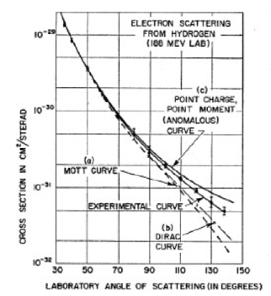
Figure 7: Angular dependence of cross sections for scattering of $188$ MeV electrons. The data measure the proton charge radius to be $(0.7\pm 0.2)\times 10^{-15}$ m. (McAlister and Hofstadter 1956).

The target proton differs from an electron in several important respects. The couplings of composite particles like the proton are not predicted by the electroweak theory, nor is the anomalous magnetic moment, $(g-2)/2$, necessarily small for a composite particle. Finally, the weak couplings may have a dependence on $Q^{2}$ which reflects the finite size of the particle. Figure 7 shows data from some of the original measurements of proton structure in $\sim 200$ MeV electron scattering. The increase in angle corresponds to an increase in the $Q^{2}$ of the electromagnetic interaction. As can be seen, the experimental data do not agree with the prediction of the proton as a Dirac particle, but require not only anomalous magnetic moment but also finite-sized charge distribution to explain the suppression at high $Q^{2}$ relative to a point charge.

The full cross section for inverse beta decay is

$$\sigma(\bar{\nu}_{e}p\to e^{+}n)=\frac{G_{F}s}{\pi}\times\cos^{2}\theta_{C}\times\xi_{mass}\times\left(g_{V}^{2}+3g_{A}^{2}\right),$$ (17)

where the first term is the point-like scattering cross section result we derived for neutrino-electron scattering, the $\theta_{C}$ term takes into account the charged-current quark mixing transition from a $u$ quark to a $d$ quark, $\xi_{mass}$ is defined in Equation 16, and $g_{V}$ and $g_{A}$ are the proton form factors. As mentioned above, the proton form factors and the relevant (small) momentum transfer for this process at low energy are not predicted by the electroweak theory, and must be experimentally determined. $g_{V}$ at low momentum transfer is the electric charge of the proton, +1, and $g_{A}$ is determined by the neutron lifetime to be $-1.26$.

3.2 Deep Inelastic Scattering

Of course, another difference between a strongly bound target, such as a nucleus, and an electron is that the strongly bound target can be broken apart in the final state to create different particles. In such a case, what do we qualitatively expect to happen to the cross section?

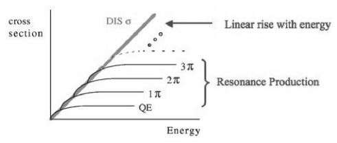
Figure 8: A schematic diagram representing the rise of the cross section with energy as inelastic channels open up with energy.

Consider first the elastic scattering process of neutrinos on nucleons. This total cross section will rise linearly with energy when the energy is sufficiently low. However, if the $Q^{2}$ of the reaction is high enough, the differential elastic cross section, $d\sigma/dQ^{2}$ will start to fall with $Q^{2}$ because the nucleon will break apart when too much $Q^{2}$ is transferred. At some point, the cross section no longer rises with energy because the elastic process only occurs up to a finite $Q^{2}$, and the $s$ at this high energy exceeds that $Q^{2}$. However, at the same point, new inelastic processes, such as the production of a single pion will become energetically possible. These will rise with energy, initially quadratically and then linearly until they too reach their $Q^{2}$ limit, at which point their cross section stops rising with energy. As illustrated in Figure 8, this process repeats itself, resulting in a linear rise of the total cross section with energy.

Of course, a linear rise with energy is exactly what is expected in the case of point like scattering. The picture above, while possibly helpful in the region of transition between elastic and inelastic to be discussed in Section 4.1, is awkward for understanding the high energy behavior of inelastic scattering. Instead, we model this process as the deep inelastic scattering of neutrinos from quarks inside the strongly bound system. These quarks are fundamental particles, and therefore the cross section of neutrino quark scattering will rise linearly with energy.

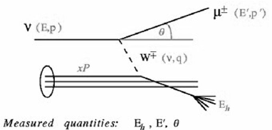
Figure 9: Kinematic quantities in deep inelastic scattering.

We first need a common language of kinematics that is relevant for an inelastic process such as $\nu N\to\ell X$ or its neutral current counterpart, $\nu N\to\nu X$. As shown in Figure 9, we define the energy and four-momentum in the lab frame of the incoming neutrino, the outgoing lepton and the weak boson, respectively, to be $p=(E,p)$, $p^{\prime}=(E^{\prime},p^{\prime})$ and $q=(\nu,q)$, and we also define the lab scattering angle of the outgoing lepton as $\theta$, the four-momentum of the target as $P$, and the energy of the hadronic recoil in the lab frame as $E_{h}$. As before we define the negative of the $W$ four-momentum squared

$$Q^{2}\equiv-q^{2}=-(p^{\prime}-p)^{2}\approx 4EE^{\prime}\sin^{2}(\theta/2).$$ (18)

Note that this definition is given purely in terms of variables on the well-defined leptonic side of the event. We will follow this convention as much as possible, expressing quantities in the lab in terms of leptonic variables and the initial target mass, $M_{T}$. We may define other invariants, such as the lab energy transfer, $\nu$, the inelasticity, $y$, and the Feynman scaling variable, $x$:

$$\nu \equiv \frac{q\cdot P}{\sqrt{P\cdot P}}=E-E^{\prime},$$

$$y \equiv \frac{q\cdot P}{p\cdot P}=\frac{\nu}{E},$$

$$x \equiv \frac{-q\cdot q}{2(p\cdot q)}=\frac{Q^{2}}{2M_{T}\nu}.$$ (19)

The center-of-mass scattering energy, $\sqrt{s}$, and the mass of the hadronic recoil system, $W$, can also be written in term of leptonic variables $x$, $y$ and $\nu$ and the target mass $M_{T}$:

$$s \equiv (p+P)^{2}=M_{T}^{2}+\frac{Q^{2}}{xy},$$

$$W^{2} \equiv (q+P)^{2}=M_{T}^{2}+2M_{T}\nu-Q^{2}.$$ (20)

In the picture of neutrinos scattering from constituents of strongly bound systems, the “parton” interpretation of deep inelastic scattering, the variable $x$ has a special interpretation as the fractional momentum of the target nucleon carried by the parton in a frame where the target momentum is very large. The common picture of this frame is that the nucleon, as seen by the incoming lepton, is flat and static because of length contraction and time dilation, and the incoming lepton interactions with a single one of these frozen partons, carrying a momentum fraction $x$. In this picture, we can define effective masses for the initial and final state partons,

$$m_{q}^{2} = x^{2}P^{2}=x^{2}M_{T}^{2},$$

$$m_{q^{\prime}}^{2} = (xP+q)^{2}$$ (21)

To make sense of deep inelastic scattering, we cannot merely consider the hard process of neutrinos scattering from quarks; we must also place those quarks inside the target hadron. This is made possible by the Factorization Theorems of QCD which allow us to write a scattering cross section for a hadronic process in terms of cross sections for scattering from partons convoluted with a parton distribution function $q_{h}(x)$:

$$\sigma(\nu+h\to\ell+X)=\sum_{q}\int dx~{}\sigma(\nu+q(x)\to\ell+X)q_{h}(x).$$ (22)

The parton distributions, while not (yet) something we can calculate from principles of QCD, are universal. Therefore, they can be determined in one process and applied to another process.

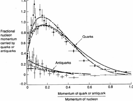
Figure 10: Distribution of quark and anti-quark momentum density in the nucleon as a function of $x$.

Figure 10 shows an illustration of typical quark and anti-quark distributions in a nucleon at moderate $Q^{2}$. The parton distribution function (PDF), $q(x)$ gives the number density of quarks of a given $x$. If quarks, carried all the momentum of the nucleon, $\int xq(x)dx=1$; however, in reality this integral is significantly less than one. This momentum sum also turns out to be logarithmically dependent on $Q^{2}$, as are the PDFs more generally. These slow changes with $Q^{2}$ are called “scaling violation”, in reference to the Feynman scaling variable, $x$. They result from the strong interactions of the quarks themselves in the nucleon. There is a duality between $Q^{2}$ and distance scales, with higher $Q^{2}$ interactions probing features at small distance scales. At these small scales, the strong interactions among partons in the nucleon will cause quarks to radiate gluons and gluons to split into quarks and anti-quarks. The net results, whose effects have been calculated quantitatively in perturbative QCD, are that quarks and anti-quarks increase in number at higher $Q^{2}$, but their average fractional momentum decreases.

3.2.1 Deep Inelastic Scattering as Elastic Neutrino-Quark Scattering

Now that we have established the link between neutrino deep inelastic scattering and elastic neutrino-quark scattering, we can apply what we have learned about elastic scattering to deep inelastic scattering. Recall that for the charged current $\nu q\to\ell q^{\prime}$ process, we expect a cross section of $G_{F}s/\pi$, up to a possible angular suppression accounting for total spin in the initial and final state. But $s=M_{T}^{2}+2M_{T}E_{\nu}$ in the lab frame. We have just learned that for each quark, the initial state target mass is $xm_{N}$, where $m_{N}$ is the nucleon mass, so the total effective target mass is of the same order of magnitude as the nucleon mass. Compared with the case of neutrino-electron scattering where the target mass was $m_{e}$, the cross section for deep inelastic scattering will be approximately three orders of magnitude larger!

We can also look at chirality and total spin in the reactions of neutrinos and quarks. Again, in the high energy limit where helicity and chirality are equivalent, consider the center-of-mass frame as we did in Figure 6. For the case of a quark, the charged-current weak interaction will pick out left-handed quarks just as it did left-handed electrons, and there will be no net spin along the interaction axis. By contrast, for the case of neutrino scattering from anti-quarks, the target will be right-handed in the center-of-mass frame, and there will be a net spin of $1$ along the interaction axis. As we argued in Equation 7, for the case of a right-handed target, the back-scattering is suppressed, and the overall cross section is reduced by a factor of three. A convenient kinematic relationship exists between the center-of-mass scattering angle, $\theta^{*}$ and the inelasticity, $y$,

$$\left(\frac{1+\cos\theta^{*}}{2}\right)=1-y,$$ (23)

and therefore, $d\sigma_{J_{z}=1}/d\theta^{*}\propto(1-y)^{2}$.

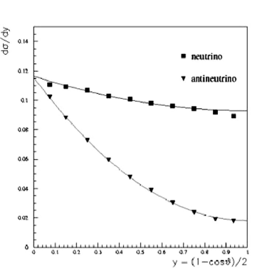
Figure 11: Neutrino and anti-neutrino deep inelastic scattering cross sections as a function of $x$.

The same argument that leads to a back-scattering or high $y$ suppression of the cross section for neutrino-antiquark scattering also holds for antineutrino-quark scattering, and similarly antineutrino-antiquark scattering has no suppression. Therefore

$$\frac{d\sigma(\nu q)}{dxdy} =\frac{d\sigma(\bar{\nu}\bar{q})}{dxdy} \propto 1,$$

$$\frac{d\sigma(\bar{\nu}q)}{dxdy} =\frac{d\sigma(\nu\bar{q})}{dxdy} \propto(1-y)^{2}.$$ (24)

This fact, combined with the smaller momentum fraction carried by antiquarks than is carried by quarks (Figure 10), means that the total anti-neutrino cross section is approximation factor of two smaller than the neutrino cross section on nucleons. Differential cross sections of each are shown in Figure 11.

3.2.2 Structure Functions in Deep Inelastic Scattering

We have approached deep inelastic scattering both from its interpretation as neutrino-quark elastic scattering, and also by purely considering the kinematics. Beyond kinematic constraints, conservation laws and Lorentz invariance also provide model independent constraints on the possible forms of inelastic scattering cross section, and in this picture, information about the structure of the target is contained in a number of general “structure functions”. If we consider the case of zero lepton mass, there are three structure functions that can be used to describe the scattering, $2xF_{1}$, $F_{2}$ and $xF_{3}$:

$$\frac{d\sigma^{\nu,\bar{\nu}}}{dxdy}\propto\left[y^{2}2xF_{1}(x,Q^{2})+\left(2-2y-\frac{M_{T}xy}{E}\right)F_{2}(x,Q^{2})\pm y(2-y)xF_{3}(x,Q^{2})\right].$$ (25)

Note that $xF_{3}$ is a structure function that is not present in electromagnetic interactions, and is only allowed because of the parity violation of the weak interaction.

There is an approximate simplification with a model of massless, free spin-$1/2$ partons, first derived by Callan and Gross, $2xF_{1}=F_{2}$. The Callan-Gross relation implies that the intermediate boson is completely transverse, and so violations of Callan-Gross are often parameterized by $R_{L}$, defined so that

$$R_{L}\equiv\frac{\sigma_{L}}{\sigma_{T}}=\frac{F_{2}}{2xF_{1}}\left(1+\frac{4M_{T}x^{2}}{Q^{2}}\right).$$ (26)

Contributions to $R_{L}$ arise because of processes internal to the target, like gluon splitting $g\to q\bar{q}$ which are calculable in perturbative QCD, and because of the target mass, $M_{T}$

Continuing with the assumptions of the validity of the Callan-Gross relation and of massless targets, we can match the $y$ dependence of the structure functions with the $y$ dependence of elastic scattering from quarks and anti-quarks to make assignments of structure functions with parton distributions. In this limit, the coefficient in front of $xF_{3}$ simplifies to $1-(1-y)^{2}$, and the coefficient multiplying $2xF_{1}=F_{2}$ is $1+(1-y)^{2}$. From Equation 24, the former would be associated with the non-singlet contribution of $q-\bar{q}$ and the later with the sum $q+\bar{q}$. Furthermore, for the charged-current, there is a charge selection, namely, a neutrino cannot produce a quark or anti-quark by sending its $W^{+}$ to a target quark unless that target quark has negative charge; otherwise, the resulting final state would have to have charge greater than $+1$ and would not be a quark. Putting all these constraints together, we find:

$$2xF_{1}^{\nu p,~{}{\rm\textstyle CC}} = x\left[d_{p}(x)+\bar{u}_{p}(x)+s_{p}(x)+\bar{c}_{p}(x)\right],$$

$$xF_{3}^{\nu p,~{}{\rm\textstyle CC}} = x\left[d_{p}(x)-\bar{u}_{p}(x)+s_{p}(x)-\bar{c}_{p}(x)\right],$$ (27)

where $q_{p}(x)$ refers to the PDF of a given quark flavor in the proton and where the contribution from third generation quarks, which have very small PDFs, is neglected.

Just as with the neutrino-electron scattering, the neutral current case is more complicated because the neutral current couples to quarks of both helicities with a non-trivial coupling constant. However, unlike the charged-current case, there is no selection based on quark charge. The neutral current structure functions under the same assumptions are:

$$2xF_{1}^{\nu p,~{}{\rm\textstyle NC}} = x\left[\left(u_{L}^{2}+u_{R}^{2}\right)\left(u_{p}(x)+\bar{u}_{p}(x)+c_{p}(x)+\bar{c}_{p}(x)\right)\right.$$

$$\left.+\left(d_{L}^{2}+d_{R}^{2}\right)\left(d_{p}(x)+\bar{d}_{p}(x)+s_{p}(x)+\bar{s}_{p}(x)\right)\right],$$

$$xF_{3}^{\nu p,~{}{\rm\textstyle NC}} = x\left[\left(u_{L}^{2}+u_{R}^{2}\right)\left(u_{p}(x)-\bar{u}_{p}(x)+c_{p}(x)-\bar{c}_{p}(x)\right)\right.$$ (28)

$$\left.+\left(d_{L}^{2}+d_{R}^{2}\right)\left(d_{p}(x)-\bar{d}_{p}(x)+s_{p}(x)-\bar{s}_{p}(x)\right)\right],$$

where the new notation here, e.g., $u_{L,R}$, refers to the left and right-handed neutral current couplings of up or down type quarks.

Some simplification in the case of the charged-current can be obtained for the practical case where the target material consists of an isoscalar nucleus with equal numbers of neutrons and protons. The light PDFs of the neutron are standardly assumed to be related to the PDFs of the proton by isospin symmetry,

$$u_{p}(x) = d_{n}(x),$$

$$d_{p}(x) = u_{n}(x),$$ (29)

and the PDFs of the heavy quarks, $s(x)$ and $c(x)$ are assumed to be identical in neutrons and protons and identical with their anti-quark distributions since they result from gluon splitting and not the valence quark content of the nucleon. Under these assumptions,

$$2xF_{1}^{\nu N,~{}{\rm\textstyle CC}} = x\left[u(x)+d(x)+\bar{u}(x)+\bar{d}(x)+2s(x)+2c(x)\right]$$

$$= x(q(x)+\bar{q}(x)),$$

$$xF_{3}^{\nu N,~{}{\rm\textstyle CC}} = x\left[u(x)+d(x)-\bar{u}(x)-\bar{d}(x)+2s(x)-2c(x)\right]$$ (30)

$$= x(q_{val}(x)+2s(x)-2c(x))$$

where the PDFs written are those of the proton and where $q_{val}(x)\equiv q(x)-\bar{q}(x)$. Note the particularly simple forms, these structure functions have, at least in the limit of neglecting the heavy quarks.

3.2.3 $\nu_{\tau}$ Charged Current Interactions

A challenging endeavor to apply our theory of deep inelastic scattering is $\nu_{\tau}$ appearance experiments such as OPERA. The full calculation of lepton mass effects is beyond the scope of these lectures. Note that all that has preceded this, including the definitions of the structure functions, assumed massless leptons. But again, we can apply our mass suppression formalism to get an approximation of the effect.

Figure 12: Mass suppression of $\nu_{\tau}$ deep inelastic scattering cross sections (Kretzer and Reno 2002).

As we argued in Equation 11, the generic form of the mass suppression is $(1-m_{final}^{2}/s)$. Since deep inelastic scattering is neutrino-quark elastic scattering, the relevant quantity for $s$ here is the $s$ of the neutrino-quark system, which is $\hat{s}=xs$. The form of the mass suppression for $\tau$ production from a given parton $x$ is then $1-m_{\tau}^{2}/(xs)$. This implies that at low $x$ the mass suppression will be large at much higher energies than at high $x$, and thus qualitatively, the rise of the cross section relative to muon neutrino charged current scattering will be very slow. This can be seen in the full calculation illustrated in Figure 12.

3.2.4 Charm Production by Neutrinos

Another way that massive final state corrections can enter into deep inelastic scattering is the production of charm quarks in neutrino deep inelastic scattering. Although there are few charm quarks to be found in the proton itself (after all, $m_{c}>m_{p}$), the sea has a large number of strange quarks, roughly half as many as either of the light quark species. Since the Cabibbo-favored charged-current process turns these strange quarks into charm quarks, production of charm quarks is a significant fraction of the charged-current cross section.

Let’s return to the kinematic variables of Equation 19 to study the effect of the final state quark mass. Production of a charm quark in the final state implies that $m_{c}^{2}=(q+\xi P)$, where $\xi$ represents the fractional momentum of the initiating quark instead of the usual Feynman scaling variable $x$. If $\xi\ll 1$, then

$$\xi\approx\frac{-q^{2}+m_{c}^{2}}{2P\cdot q}=\frac{Q^{2}+m_{c}^{2}}{2M_{T}\nu}=x\left(1+\frac{m_{c}^{2}}{Q^{2}}\right).$$ (31)

The reason introducing $\xi$ as distinct from $x$ now becomes obvious. The $x$ variable as defined in terms of leptonic side variables is no longer the same as the fractional momentum carried by the target quark, but is in fact smaller. Therefore, for a given set of scattering kinematics, the initiating quark must carry a higher fractional momentum and thus will be less common than in the case where a light quark is produced in the final state. This formalism for treating the production of massive quarks is referred to as “slow rescaling”.

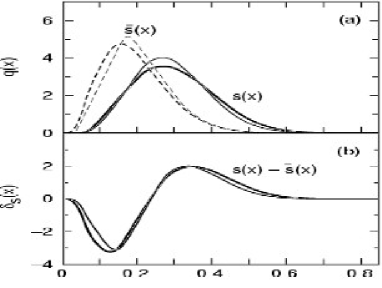
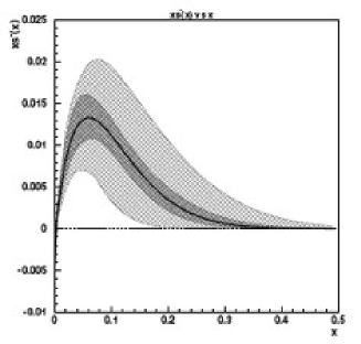
Figure 13: Non-perturbative model of Brodsky and Ma for $s(x)-\bar{s}(x)$ (left) compared with data from NuTeV (right).

One of the best ways to actually measure the strange quark content of the nucleon is to measure charged-current charm quark production tagged by the semi-muonic decay of charm in a neutrino experiment. In other words, determine $s(x)$ by measuring $\nu_{\mu}+s\to\mu^{-}+c+X$, $c\to\mu^{+}+X$ and its anti-neutrino analog, each of which give two high momentum muons in the final state and are commonly referred to as “dimuon” events.

There is currently some debate about parton distributions regarding whether the strange and anti-strange seas carry equal momentum. Strange quarks and anti-quarks generated by perturbative processes should be nearly symmetric in momentum, but there are non-perturbative effects that can lead to differences in their momentum. The NuTeV experiment has recently completed an analysis of dimuon events induced by neutrino beams and anti-neutrino beams which therefore separately measure the strange and anti-strange quark distributions in the nucleus. Figure 13 shows a comparison of one theoretical prediction with the measurement of this momentum asymmetry from NuTeV.

4 Transitions between Elastic and Inelastic Scattering

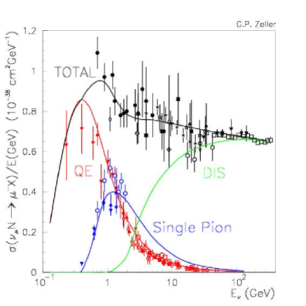
Figure 14: A compilation of neutrino cross sections, shown as $\sigma/E_{\nu}$, in the GeV region with quasi-elastic, deep inelastic and single pion cross sections shown separately. (Figure courtesy G.P. Zeller).

To this point, we have explored elastic scattering of neutrinos from pointlike particles and a high energy limit of neutrinos scattering inelastically from nucleons where the neutrino effectively scatters from free quarks in the target. If we look at the cross sections shown in Figure 14, we see both the elastic and deeply inelastic cross sections co-existing over a broad region with a significant component over nearly an order of magnitude in energy being the “barely inelastic” process of single pion production. This transition occurs at these energy values because the “binding energy” of the the target nucleon is approximately $\lambda_{QCD}$, which is the scale of a typical momentum exchange for scattering of a neutrino with $1$ GeV energy.

This section of the lectures will explore a few features of regions of transition. Because it is of the most interest for oscillations, we will largely focus on the transition between nucleon elastic and inelastic at neutrino energies near a GeV, but we will conclude with comments on other transition regions of interest.

4.1 The GeV Region

We have exhaustively described the deep inelastic scattering limit of Figure 14, but have not spent much time describing the quasi-elastic cross section, e.g. $\nu_{\mu}n\to\mu^{-}p$. At low energies, we expect by the same arguments given in other cases of lepton mass, a suppression due to the muon mass going roughly as

$$\frac{\sigma}{\sigma_{\rm\textstyle massless}} \sim 1-\frac{(M_{T}+m_{\mu})^{2}}{s}$$ (32)

$$= 1-\frac{M_{T}^{2}+2M_{T}m_{\mu}+m_{\mu}^{2}}{M_{T}^{2}+2E_{\nu}M_{T}}$$

$$\approx \frac{2E_{\nu}}{M_{T}}~{}~{}~{}{\rm\textstyle if}~{}E_{\nu}<<M_{T}.$$

Thus the cross section at low energies will be quadratic until $E_{\nu}\sim m_{T}/2$, as shown in Figure 14. However, we also see that the cross section stops growing above $E_{\nu}\sim 1$ GeV. As we observed in Section 3.2, above a sufficiently high $Q^{2}$, $d\sigma/dQ^{2}$ begins to fall because interactions at higher $Q^{2}$ tend to break apart the target nucleon and therefore are not quasi-elastic.

Nucleon structure also plays a significant role in quasi-elastic scattering. As with deep inelastic scattering, it is relatively straightforward to write a cross section formula for quasi-elastic scattering; however, in the end there are unknown form factors that enter the calculation which must be determined experimentally. The cross section is usually parameterized in terms of vector, $F_{V}$, and axial vector form factors, $F_{A}$,

$$F_{V,A}\approx\frac{F_{V,A}(0)}{\left(1+Q^{2}/M_{V,A}^{2}\right)^{2}},$$ (33)

in the so-called “dipole approximation” (Llewellyn Smith 1972). These are only phenomenological approximations to the true form factors, and precise measurements of the vector form factor $F_{V}$ in electron scattering show significant deviations from the dipole form at $Q^{2}\gg M_{V}^{2}$ where $M_{V}\approx 0.84$ GeV. The axial vector form factor parameters are well determined only at $Q^{2}\approx 0$ (recall the discussion following Equation 17), and the best current estimates from data of the axial mass give $M_{A}\approx 1.1$ GeV with significant theoretical and experimental uncertainties.

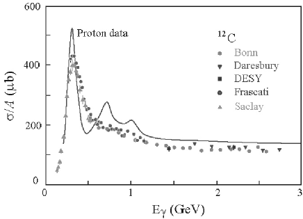
Figure 15: Photo-absorption data on protons (line) and nuclei (data points) as a function of energy illustrating the effect of Fermi smearing on resonance production.

As the cross section becomes barely inelastic, this region is often called the “resonance region” because it is dominated by the production of discrete baryon resonances in the final state. Recall that the mass of the hadronic system, $W$, is given by $W^{2}=M_{T}^{2}+2M_{T}\nu(1-x)$. In the barely inelastic regime, this cannot take any arbitrary value because there must be a baryonic state available at that mass. As the solid line in Figure 15 illustrates in a different process, photo-nuclear absorption, there are discrete excitation lines corresponding to specific broad baryon resonances. The lowest mass excited baryonic state is the $\Delta(1232)$ resonance which is very visible and separated as the first peak in Figure 15. Above the $\Delta(1232)$, resonances tend to overlap one another and approach a continuum.

How is it possible to understand such a complicated set of overlapping final states? One way to gain a good qualitative and the beginning of a quantitative understanding is through Bloom-Gilman duality. The ideal of duality is that, on average, one can model the behavior of discrete hadronic states through the behavior of their underlying quark content. This emperically successful idea straddles the border between asymptotically free and confined states in QCD.

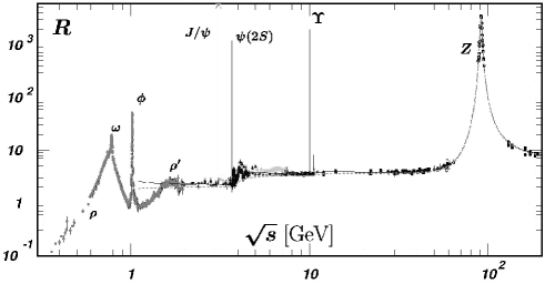
Figure 16: The ratio of $e^{+}e^{-}$ annihilation cross section into hadrons divided by that into muons

.

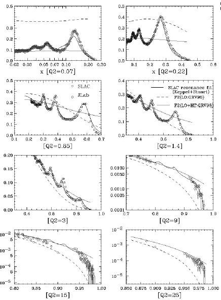
Figure 17: Electron scattering data in the baryon resonance region compared to a quark-model calculation (Bodek and Yang 2002).

The most famous example of Bloom-Gilman duality is illustrated in the quantity $R=\sigma(e^{+}e^{-}\to$ hadrons$)/\sigma(e^{+}e^{-}\to\mu^{+}\mu^{-})$. Shown in Figure 16 is $R$ compared against a prediction from the quark model that $R=N_{C}\sum Q_{q}^{2}$, where $Q_{q}$ and $N_{C}$ are the charge and number of color states for the quark, respectively. The sum runs over all quark states that can be produced at a given $s$. This method works well to describe the cross-section over a complicated mix of final states that can be found well above the $s\bar{s}$ ($\phi$) threshold, and also in the region above the $c\bar{c}$ and $b\bar{b}$ narrow resonances.

Duality has also been applied successfully to describe the resonance region in electron scattering data (Bodek and Yang 2002), and a comparison of a quark model with actual electron scattering data is shown in Figure 17. The resonance structure essentially appears as modulations on top of the quark model prediction. This approach is now being used in most modern neutrino generators attempting to interpolate the region of hadronic mass squared, $W^{2}$, best treated as production of discrete resonances and the higher energy region where parton model calculations of deep inelastic scattering are good approximations.

4.2 The Effect of the Nucleus

A significant complication for the understanding of neutrino interactions in future experiments is the need to model cross sections on a variety of nuclei. Exclusive neutrino interactions in the GeV energy range of the type that must be understood in future experiments are particularly sensitive to modification in the nuclear medium, and there are few definitive models and little data currently available to help to understand the effects. In this section, we will survey some of the relevant phenomenology.

One effect that is relevant for all energy regimes is the motion of the target nucleon to the nucleus. This is often called “Fermi smearing”, and it can have a dramatic effect. Figure 15 illustrates how significant this effect is on the production of resonances in photo-nuclear absorption. The proton data represented by the solid line clearly shows multiple resonance peaks, but in ${}^{12}C$, the same resonances become indistinct due to Fermi smearing except for the well separated $\Delta(1232)$ resonance. Similar dramatic effects can be seen in reconstruction of quasi-elastic events, and in scattering from high $x$ partons in deep inelastic scattering.

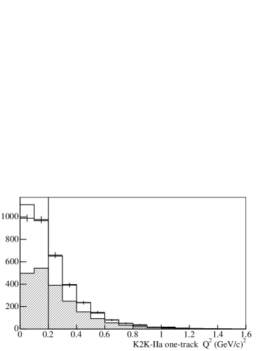
Figure 18: $Q^{2}$ distribution in a quasi-elastic enriched sample in the SciBar detector at KEK (Gran 2006) shown for two different running periods. The estimation of the number of events due to quasi-elastic processes in each bin is shown by the shaded area.

Quasi-elastic scattering at low $Q^{2}$ has a unique nuclear effect. Because the final state nucleon will not necessarily be energetic enough to leave the nucleus, its creation may be suppressed if there is no free nuclear state available due to the Pauli exclusion principle. This effect is often called Pauli blocking. The effect can be modeled, although it is unclear how well these models work or how universal they are. Even with a model for Pauli blocking in their predictions, both the SciBar and MiniBooNE detectors see significant deficits of events from scattering off of carbon at low $Q^{2}$ (Figure 18).

Another significant effect is the rescattering in the nuclear medium of hadrons which are sufficiently energetic to escape the target nucleus. Because the nucleus is so dense, the material traversed when a produced particle escapes the target nucleus is significant compared to the amount of nuclear matter it sees when traveling through macroscopic amounts of detector material afterward. Therefore, it is not surprising that the probability of a reinteraction in the nucleus is significant. Such a reinteraction may be particularly difficult for an experiment relying on knowledge of exclusive final states, such use of two-body kinematic constraints in reconstructing quasi-elastic events, or when concerned about backgrounds to $\nu_{e}$ appearance from $\pi^{0}$s. Again, these effects are not well studied, although there is some promise in the use of electron scattering data to constrain models of such final state reinteractions.

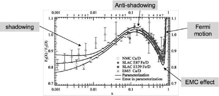
Figure 19: Nuclear effects on parton distributions.

In the deep inelastic scattering region, nuclear effects are well measured in charged lepton scattering and are often parameterized in terms of their effect on parton distribution functions as shown in Figure 19. At high $x$, the same Fermi smearing described above leads to a dramatic increase in the rare partons carrying very high $x$. The region of moderate $x$, in the “valence quark” region is suppressed through an effect generally named the “EMC” effect after the first experiment to observe it. At $x\sim 0.1$, there is a small enhancement of the PDFs sometimes referred to as “anti-shadowing” and PDFs at low $x$ appear to be dramatically suppressed due to “shadowing”. Because these effects have only been measured in charged-lepton scattering and because, with the exception of the Fermi smearing and perhaps shadowing, there are plausible but not definitive theoretical interpretations of the effect, it is not clear whether the modifications to PDFs are in fact universal, or whether the effects in neutrino neutral and charged-current scattering will be different. Most likely, data from neutrino scattering experiments on a variety of nuclei, including light nuclei, will be required to resolve this question.

4.3 Other Regimes of Transition

There are other regions of transition, usually associated with binding thresholds. Binding energies of electrons in atoms are $\stackrel{{\scriptstyle<}}{{\sim}}Z^{2}m_{e}c^{2}\alpha_{E}M$ which can cover a broad range in energy from a few eV to $10^{5}$ eV, and certainly at very low energies these bindings can affect neutrino scattering from atomic electrons. However, this is not in an energy range that has effected neutrino oscillation experiments to date. There is also a transition region associated with the binding energy of nucleons inside the nucleus that ranges from $0.1$–$10$ MeV. This binding energy most definitely has had an impact on oscillation physics in a number of experiments. The SNO experiment uses charged and neutral-current reactions $\nu_{e}d\to ppe^{-}$ and $\nu d\to pn\nu$ on deuterons and elastic scattering from atomic electrons as its oscillation signatures. For the few MeV neutrinos from the sun, the thresholds of atomic electrons, $<1$ keV even for oxygen, are irrelevant. However, the $2.2$ MeV binding energy of the deuteron and the characteristic sharp quadratic turn-on with neutrino energy at the threshold is a significant theoretical uncertainty in reaction rates for low energy neutrinos.

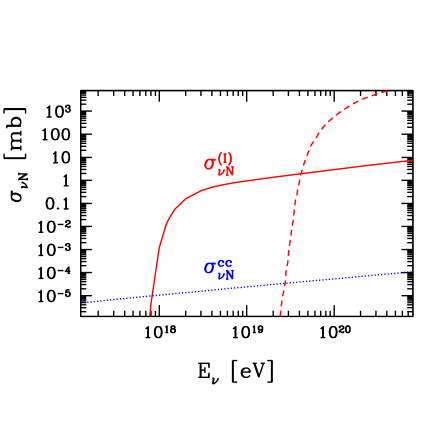
Figure 20: Possible modifications of ultra-high neutrino energy cross sections could be quite dramatic if new degrees of freedom can be excited at high energies. This model (Fodor 2003) shows an example using electroweak instantons.

A more interesting possibility might be realized in cosmic ray physics involving neutrinos. Although our current knowledge from energy frontier colliders limits the energy scale at which quarks and leptons might be bound states to $\stackrel{{\scriptstyle>}}{{\sim}}10$ TeV, beyond this it is possible that some new process turns on as illustrated in Figure 20. It is interesting to remember from our discussions that the “background” deep inelastic cross section will continue to grow with energy approximately linearly until $Q^{2}>M_{W}^{2}$, when the propagator term (Equation 3) will begin to drop with increasing $Q^{2}$. This effect begins to be noticeable at neutrino energies of $\sim 10$ TeV, and is so significant at high energies that baseline “QCD” cross section in Figure 20 is barely increasing with energy.

5 Conclusions

By way of conclusions, I will offer in compact form what I think are the most important points for the student to take away from these lecture notes.

The understanding of neutrino interactions is one of the keys to precision measurements of neutrino oscillations at accelerators. It will soon limit precision in the current program of $\nu_{\mu}$ disappearance at atmospheric baselines. In the future cross section uncertainties, if not addressed with new data, will play a significant role in the ultimate precision of the $\nu_{\mu}\to\nu_{e}$ and $\bar{\nu}_{\mu}\to\bar{\nu}_{e}$ measurements needed to untangle the neutrino mass hierarchy and to search for leptonic CP violation.

The neutrino scattering rate is generally proportional to energy. Specifically this is true for scattering from pointlike particles when the $Q^{2}\ll M_{W}^{2}$. When it is not true for an exclusive process below this $Q^{2}$ threshold, then there is some physics limiting the maximum momentum transfer, such as a threshold above which the target breaks up.

Neutrino target structure (atom, nucleus, nucleon) is a significant complication to precise theoretical calculation of cross section on neutrinos, particularly near inelastic thresholds. Tools like quark-hadron duality are helpful for modeling the major features, but detailed predictive models require additional data we do not currently have in hand, particularly when knowledge of the nuclear environment is needed to make a firm prediction.

Acknowledgments

I am grateful to the organizers of summer school for providing a stimulating environment and program of study and for their hard work in recruiting students to the school. I thank in particular Franz Muheim for his thoughtful and careful review and editing of this manuscript. I also thank Dave Casper, Rik Gran, Debbie Harris, Jorge Morfin, Tsuyoshi Nakaya and Sam Zeller for providing material for or useful comments on the lectures on which this manuscript is based.

References

Bethe, H. and Peierls, R. (1934), Nature 133, 532.

Bodek, A. and Yang, U.-K. (2002), Nucl. Phys. Proc. Suppl. 112 70.

Fermi, E. (1934), Z. Physik 88, 161.

Fodor, Z. et al. (2003), Phys. Lett. B561 191.

Galison, P. (1983), Rev. Mod. Physics 55, 477.

Gran, R. et al. (2006), Phys. Rev. D74, 052002.

Kretzer, S. and Reno, M.H. (2002), Phys. Rev. D66 113007.

Llewellyn Smith, C.H. (1972), Phys. Rep. 3C, 261.

McAlister, R. and Hofstadter, R. (1955), Phys. Rev. 102 851.

Minakata, H. and Nunokawa, H. (2001), Jour. HEP 0110 001.

Reines, F. (1996), Rev. Mod. Physics 68 317.

Sterman, G. et al. (1995), Rev. Mod. Physics 67, 157.

Zeller, G.P. (2003), arXiv:hep-ex 0312061.