Modelling coloured residual noise in gravitational-wave signal processing

Abstract

We introduce a signal processing model for signals in non-white noise, where the exact noise spectrum is a priori unknown. The model is based on a Student’s $t$ distribution and constitutes a natural generalization of the widely used normal (Gaussian) model. This way, it allows for uncertainty in the noise spectrum, or more generally is also able to accommodate outliers (heavy-tailed noise) in the data. Examples are given pertaining to data from gravitational wave detectors.

1 Introduction

The measurement of gravitational radiation holds great promise for exciting astronomical observations [1, 2]. Around the world, efforts are under way to construct and improve detectors for gravitational waves; among these are the LIGO detectors in the US [3], GEO [4] and Virgo [5] in Europe, and TAMA in Japan [6], some of which have already started taking data. Plans for future detectors include advanced LIGO [7], LCGT in Japan [8], the Laser Interferometer Space Antenna (LISA) [9] and the Einstein Telescope (ET) [10]. As existing instruments are becoming increasingly sensitive and future instruments are approaching completion, sophisticated signal processing methods are required in order to detect and accurately interpret these often weak signals within a noisy environment. For example, signal detection is usually implemented via matched filtering [11, 12, 13], while parameter estimation is commonly done using Bayesian methods [14, 15]. Many of the data analysis procedures employed to date are based on the assumption of the noise being Gaussian with a known power spectral density [11, 16]. While these methods have proven to be computationally efficient and very powerful at discriminating rare, weak signals within noise, some more flexibility or robustness is sometimes desired. One example is the analysis of data to be expected from LISA, where the measurement noise originates partly from instrumental as well as astrophysical sources, and the noise spectrum is only vaguely known a priori [17].

We introduce an approach that was developed in the context of the latter case, where, along with the signal parameters to be inferred, the noise’s power spectrum needed to be incorporated as an unknown into the model [18, 19]. The model developed here turns out to be computationally convenient, as the additional noise parameters may be analytically integrated out, leading to a Student-$t$ likelihood expression instead of the original normal formulation. We expect the same approach to be useful in many related signal processing contexts, as it allows to specify the prior information about the power spectrum, i.e., its expected magnitude and the associated certainty, in a straightforward manner. In this way, it should e.g. also be able to account for nonstationarities in the data, in the sense that the power spectrum does not necessarily need to be assumed to be exactly the same as at an earlier measurement; other fluctuations, like outliers, could also be accommodated in a similar manner. In fact, the resulting model actually falls into a class of generalizations to the standard Gaussian that have been proposed for their robustness properties: models accommodating heavier-tailed noise, or outliers, by either (‘directly’) implementing a non-Gaussian noise model or (‘indirectly’) substituting the corresponding least-squares procedures by less outlier-sensitive methods. Instead of the derivation based on an unknown power spectrum, the same model may be motivated by assuming the power spectrum itself to be random, so that the resulting noise mixture distribution exhibits a greater variability. In the limiting case of decreasing spectrum variability, the model again simplifies to the Gaussian. So the model will also be applicable as an ad-hoc alternative tunable robust model, with clearly interpretable “tuning parameters”.

The organization of the paper is as follows. The time series setup is introduced in Section 2.1. In the subsequent sections, the probabilistic modelling is described, including its time-domain counterpart, the likelihood, prior distributions, posterior distribution, marginal likelihood and some implications. Section 3 describes the approach using two illustrative examples of simulated time series with and without a signal. The discussion section 4 puts the new approach into context. An appendix explicating the Discrete Fourier Transform conventions used in this paper is attached.

2 The time series model

2.1 The setup

Consider a time series $x_{1},\ldots,x_{N}$ of $N$ real-valued observations sampled at constant time intervals $\Delta_{t}$, so that each observation $x_{i}$ corresponds to time $t_{i}=i\Delta_{t}$. This set of $N$ observations can equivalently be expressed in terms of sinusoids of the Fourier frequencies:

$$x_{i}=\frac{1}{\sqrt{N\Delta_{t}}}\sum_{j=0}^{\lfloor N/2\rfloor}a_{j}\cos(2\pi f_{j}t_{i})+b_{j}\sin(2\pi f_{j}t_{i})$$ (1)

where the variables $a_{j}$ and $b_{j}$ each correspond to Fourier frequencies $f_{j}=j\Delta_{f}=\frac{j}{N\Delta_{t}}$. The summation in (1) runs from $j=0$ to $j=\lfloor N/2\rfloor$, with $\lfloor N/2\rfloor$ denoting the largest integer less than or equal to $N/2$. By definition, $b_{0}$ is always zero, and $b_{\lfloor N/2\rfloor}$ is zero if $N$ is even; going over from $x_{i}$’s to $a_{j}$’s and $b_{j}$’s again yields the same number ($N$) of non-zero figures. The set of ($N$) frequency domain coefficients $a_{j}$ and $b_{j}$ and the time domain observations $x_{i}$ are related to each other through a discrete Fourier transform (and appropriate scaling; see the appendix). The set of trigonometric functions in (1) constitutes an orthonormal basis of the sample space, so that there is a unique one-to-one mapping of the observations in time and in frequency domain. Instead of the two amplitudes $a_{j}$ and $b_{j}$, the definition in (1) may equivalently be expressed in terms of a single amplitude and a phase parameter at each frequency:

$$x_{i}\;=\;\frac{1}{\sqrt{N\Delta_{t}}}\sum_{j=0}^{\lfloor N/2\rfloor}\lambda_{j}\,\sin(2\pi f_{j}t_{i}+\varphi_{j}),$$ (2)

where $\lambda_{j}=\sqrt{a_{j}^{2}+b_{j}^{2}}$ and

$$\varphi_{j}=\left\{\begin{array}[]{ll}\arctan\Bigl{(}\frac{b_{j}}{a_{j}}\Bigr{)}&\mbox{if }a_{j}>0\\[4.30554pt] \arctan\Bigl{(}\frac{b_{j}}{a_{j}}\Bigr{)}\pm\pi&\mbox{if }a_{j}<0.\end{array}\right.$$

For each Fourier frequency $f_{j}$, let $\kappa_{j}$ be the number of Fourier coefficients not being zero by definition, i.e.:

$$\kappa_{j}=\left\{\begin{array}[]{ll}1&\mbox{if }(j=0)\mbox{ or }(N\mbox{ is even and }j=N/2)\\ 2&\mbox{otherwise}\end{array}\right.$$ (3)

so that $\sum_{j=0}^{\lfloor N/2\rfloor}\kappa_{j}=N$. Note that generally one may often simplify to $\kappa_{j}\!=\!2\;\forall j$ without introducing a noticeable discrepancy, but in the following we will stick to the accurate notation of $\kappa$ depending on the index $j$.

For a given time series (either in terms of $x_{i}$ or $a_{j}$ and $b_{j}$), we define the functions of the Fourier frequencies

$$p_{1}(f_{j}) = \frac{a_{j}^{2}+b_{j}^{2}}{\kappa_{j}}\qquad\mbox{and }$$ (4)

$$p_{2}(f_{j}) = \frac{a_{j}^{2}+b_{j}^{2}}{\kappa_{j}^{2}}\;=\;\frac{p_{1}(f_{j})}{\kappa_{j}}\;=\;{\textstyle\frac{\Delta_{t}}{N}}\,|\tilde{x}(f_{j})|^{2}$$ (5)

for $j=0,\ldots,\lfloor N/2\rfloor$, where $\tilde{x}$ denotes the discretely Fourier-transformed time series $x$, as defined in the appendix. These are the empirical, discrete analogues of the one-sided and two-sided spectral power. The set of $p_{1}(f_{j})$ is also known as the periodogram of the time series [20].

Now consider the case where the observations $x_{i}$, and consequently the $a_{j}$ and $b_{j}$, correspond to random variables $X_{i}$, $A_{j}$ and $B_{j}$, respectively. This may mean that these are realizations of a random process, where the random variables’ probability distributions describe the randomness in the observations, or that they are merely unknown, where the probability distributions describe a state of information, or it may also be a mélange of both [21].

The time series has a zero mean if and only if the expectation of all frequency domain coefficients is zero as well:

$$\mathrm{E}[X_{i}]=0\quad\forall i\qquad\Leftrightarrow\qquad\mathrm{E}[A_{j}]=\mathrm{E}[B_{j}]=0\quad\forall j.$$ (6)

For the probabilistic time series, the spectral power ($p_{1}(f_{j})$ or $p_{2}(f_{j})$) consequently also is a random variable ($P_{1}(f_{j})$ or $P_{2}(f_{j})$, respectively). We denote its expectation value by $S^{\ast}(f_{j})$; if the mean is zero as in (6), it is given by

$$S^{\ast}_{1}(f_{j})=\textstyle\kappa_{j}S^{\ast}_{2}(f_{j})=\mathrm{E}[P_{1}(f_{j})]=\mathrm{E}\Bigl{[}\frac{A_{j}^{2}+B_{j}^{2}}{\kappa_{j}}\Bigr{]}\stackrel{{\scriptstyle\mbox{\small(\ref{eqn:zeromean})}}}{{=}}\textstyle\frac{\mathrm{Var}(A_{j})+\mathrm{Var}(B_{j})}{\kappa_{j}}.$$ (7)

It is important to note that while the above expectation is closely related to a time series’ power spectral density, it is yet quite different. Up to here we have considered the discretely Fourier transformed data and some of its basic properties. The figure $S^{\ast}(f_{j})$ refers to data sampled at a particular resolution and sample size and is defined only at a discrete set of Fourier frequencies $f_{j}$. One might want to refer to $S^{\ast}$ as the discretized power spectrum. If in fact the data are a realization from a stationary random process with (continuous) power spectral density $S(f)$, then the expectation $S^{\ast}(f_{j})$ is related to $S(f)$ through a convolution, depending on the sample size $N$. Only in the limit of an infinite sample size both of them are equal [20, 22]. While both continuous and discretized spectrum are commonly used as an approximation to or in place of one another, it is crucial to realize that in the following inference will be done with reference to the case of a finite sample size and the discretized, convolved spectrum $S^{\ast}(f_{j})$.

A related useful figure in this context is the integrated spectrum with respect to some frequency range $[f_{1},f_{2}]$ [23], which here we define as

$$\mathcal{I}_{[f_{1},f_{2}]}=\Delta_{f}\sum_{j=j_{1}}^{j_{2}}\frac{\kappa_{j}}{2}\,S^{\ast}_{1}(f_{j})$$ (8)

where the summation is done over the corresponding range of Fourier frequencies ($j_{1}=\min\{k:f_{k}>f_{1}\}$, $j_{2}=\max\{k:f_{k}\leq f_{2}\}$, where $f_{2}-f_{1}\geq\Delta_{f}$). The integrated spectrum allows to investigate or compare (discrete) spectra independent of the particular sample size $N$.

2.2 The normal model

Suppose the moments as defined in (6) and (7) are given. We may set up a corresponding normal time series model by assuming all the (frequency domain) observables to be stochastically independent, have zero mean and

$$\mathrm{Var}(A_{j}) = \sigma_{j}^{2},$$ (9)

$$\mathrm{Var}(B_{j}) = (\kappa_{j}-1)\,\sigma_{j}^{2}\quad\mbox{for }j=0,\ldots,\lfloor N/2\rfloor,$$ (10)

where

$$\sigma_{j}^{2}\;=\;\textstyle S^{\ast}_{1}(f_{j})\;=\;\textstyle\kappa_{j}\,S^{\ast}_{2}(f_{j})\quad\mbox{for }j=0,\ldots,\lfloor N/2\rfloor.$$ (11)

While other choices of variance settings matching the assumptions would be possible, the assumption of equal variances for $A_{j}$ and $B_{j}$ is the only one that makes the joint density of $(A_{j},B_{j})$ a function of overall amplitude $\lambda_{j}$ alone, independent of the phase $\varphi_{j}$, and with that leaves the model invariant with respect to time shifts. The same model may also be motivated via the maximum entropy principle, as the (zero mean, equal variance, independent) normal distribution maximizes the entropy given the constraints on the moments given in (6) and (7) above [24]. In that way, the normal model constitutes a most convervative model setup under the given assumptions [21, 22, 24].

The joint normal distribution derived here has actually been commonly used before (see e.g. [25]); the normality assumption may not only appear as a natural choice, but will also turn out computationally convenient in the following. In the context of Fourier domain data in particular, the normality assumption may also be motivated via asymptotic arguments, by considering the limit of an infinite observation time [26, 27, 28]. The resulting normal model also is exactly the same as the one underlying the so-called Whittle likelihood [29, 30], or the one at the basis of matched filtering [11, 12, 13]. While intuitively in other contexts it may often be sufficient to point out the asymptotic equality $S^{\ast}(f_{j})\approx S(f_{j})$ for $N\rightarrow\infty$, here it is crucial to appreciate what exactly the $\sigma_{j}^{2}=\textstyle S^{\ast}_{1}(f_{j})$ stand for in the case of a finite sample size $N$. The difference between the exact and approximate (“Whittle”) model is explicated in more detail in [30].

2.3 The corresponding time-domain model

An immediate consequence of the normality assumption for the frequency-domain coefficients ($A_{j}$, $B_{j}$) is that the time-domain variables ($X_{i}$), being linear combinations of the frequency-domain variables, also follow a normal distribution. The exact joint distribution of the $X_{i}$ is completely determined by their variance/covariance structure, which may be expressed in terms of the autocovariance function. The covariance for any pair of time-domain observations $X_{m}$ and $X_{n}$ (with $m,n\in\{1,\ldots,N\}$, and corresponding to times $t_{m}$ and $t_{n}$) is given by:

$$\mathrm{Cov}(X_{m},X_{n})\\ \;=\;\frac{1}{N\Delta_{t}}\sum_{j=0}^{\lfloor N/2\rfloor}\left(S^{\ast}_{1}(f_{j})\,\textstyle\frac{\kappa_{j}}{2}\,\cos\bigl{(}2\pi f_{j}(t_{n}-t_{m})\bigr{)}\right).$$

Note that the autocovariance $\mathrm{Cov}(X_{m},X_{n})=\gamma(t_{n}-t_{m})$ depends on $t_{m}$ and $t_{n}$ only via their time lag $t_{n}-t_{m}$. Remarkably (though not surprisingly), following either the invariance or the maximum entropy argument to motivate the model structure in section 2.2, the result is a strictly stationary model for the data [31]. Note also that $\gamma(0)=\mathrm{Var}(X_{i})=\mathcal{I}_{[0,f_{N/2}]}$.

The autocovariance function allows one to express the distribution of the $X_{i}$ in terms of their ($N\times N$) covariance matrix $\Sigma_{X}$, which is the symmetric, square Toeplitz matrix

$$\Sigma_{X}\;=\;\left(\begin{array}[]{cccccc}\gamma(0)&\gamma(\Delta_{t})&\gamma(2\Delta_{t})&\cdots&\gamma(\Delta_{t})\\ \gamma(\Delta_{t})&\gamma(0)&\gamma(\Delta_{t})&\cdots&\gamma(2\Delta_{t})\\ \gamma(2\Delta_{t})&\gamma(\Delta_{t})&\gamma(0)&\cdots&\gamma(3\Delta_{t})\\ \vdots&\vdots&\vdots&\ddots&\vdots\\ \gamma(\Delta_{t})&\gamma(2\Delta_{t})&\gamma(3\Delta_{t})&\cdots&\gamma(0)\\ \end{array}\right),$$ (12)

since $\gamma$ is periodic such that $\gamma(i\Delta_{t})=\gamma((N-i)\Delta_{t})$. The periodic formulation in (1) makes the first and last observations $X_{1}$ and $X_{N}$ “neighbours”, just as $X_{1}$ and $X_{2}$ are. This may seem odd (depending on the context, of course), but is not an unusual problem, as it arises for any conventional spectral analysis of discretely sampled data in the form of spectral leakage [32]; it may just not always be as obvious in its consequences. The above time domain expression sheds some light on the exact shortcomings of the Whittle likelihood approximation; you can see for example that it will be a poor approximation in case of predominantly low-frequency noise and a small number of observations. The problem may be tackled via windowing of the data, or it will also lessen with an increasing sample size; again, the features of this approximation are discussed in more detail in [30].

2.4 Incorporating an unknown spectrum

2.4.1 The likelihood function

Now suppose the spectrum is unknown and to be inferred from the data $x_{1},\ldots,x_{N}$. An unknown spectrum here is equivalent to the variance parameters $\sigma_{0}^{2},\ldots,\sigma_{\lfloor N/2\rfloor}^{2}$ being unknown. Assuming normality of $A_{j}$ and $B_{j}$, the likelihood function (as a function of the parameters $\sigma_{0}^{2},\ldots,\sigma_{\lfloor N/2\rfloor}^{2}$) is:

$$\;p(x_{1},\ldots,x_{N}\,|\,\sigma_{0}^{2},\ldots,\sigma_{\lfloor N/2\rfloor}^{2})$$ (13)

$$=\; \;\prod_{j=0}^{\lfloor N/2\rfloor}\Biggl{[}\frac{1}{\sqrt{2\pi}\,\sigma_{j}}\exp\Bigl{(}-\frac{a_{j}^{2}}{2\sigma_{j}^{2}}\Bigr{)}\times\Bigl{(}\frac{1}{\sqrt{2\pi}\,\sigma_{j}}\Bigr{)}^{\kappa_{j}-1}\exp\Bigl{(}-\frac{b_{j}^{2}}{2\sigma_{j}^{2}}\Bigr{)}\Biggr{]}$$

$$=\; \;\exp\Biggl{(}-{\textstyle\frac{N}{2}}\log(2\pi)-\sum_{j=0}^{\lfloor N/2\rfloor}\left[\kappa_{j}\log(\sigma_{j})+\frac{a_{j}^{2}+b_{j}^{2}}{2\sigma_{j}^{2}}\right]\Biggr{)}$$ (14)

$$\propto\; \;\exp\Biggl{(}-\sum_{j=0}^{\lfloor N/2\rfloor}\frac{\kappa_{j}}{2}\left[\log\bigl{(}S^{\ast}_{2}(f_{j})\bigr{)}+\frac{\frac{\Delta_{t}}{N}\,|\tilde{x}_{j}|^{2}}{S^{\ast}_{2}(f_{j})}\right]\Biggr{)}.$$ (15)

The term $\tilde{x}_{j}$ here denotes the $j$th element of the Fourier-transformed data vector, as defined in the appendix. The above likelihood (15) is exactly equivalent to the so-called Whittle likelihood, which is an approximate expression for stationary time series [29, 30].

If the noise spectrum is a priori known, the “$\log\bigl{(}S^{\ast}_{2}(f_{j})\bigr{)}$” term may also be irrelevant (see (29)), and the model again reduces to the normal model described e.g. in [11] that is also the basis for matched filtering [12, 13]. In that case, the logarithmic likelihood may be conveniently expressed in terms of an inner product of vectors, allowing for a geometric interpretation that is expecially useful in the case of linear signal models [11, 16, 33].

2.4.2 The conjugate prior distribution

For the model defined above, the conjugate prior distribution for each of the $\sigma_{0}^{2},\ldots,\sigma_{\lfloor N/2\rfloor}^{2}$ is the scaled inverse $\chi^{2}$-distribution with scale parameter $s_{j}^{2}$ and degrees-of-freedom parameter $\nu_{j}$:

$$\sigma_{j}^{2}\;\sim\;\mbox{Inv-}\chi^{2}(\nu_{j},s_{j}^{2})$$ (16)

with density function

$$f_{\nu_{j},s^{2}_{j}}\bigl{(}\sigma^{2}_{j}\bigr{)}\;=\;\frac{\Bigl{(}\frac{\nu_{j}\,s^{2}_{j}}{2}\Bigr{)}^{\nu_{j}/2}}{\Gamma(\nu_{j}/2)}\,\bigl{(}\sigma_{j}^{2}\bigr{)}^{-(1+\nu_{j}/2)}\,\exp\biggl{(}-\frac{\nu_{j}\,s^{2}_{j}}{2\,\sigma^{2}_{j}}\biggr{)}$$ (17)

[34]. The degrees-of-freedom here denote the precision in the prior distribution, while the scale determines its order of magnitude. For increasing $\nu_{j}$ the distribution’s variance goes towards zero, and for $\nu_{j}\rightarrow 0$ the density converges toward the non-informative (and improper) distribution with density $f(\sigma_{j}^{2})=\frac{1}{\sigma_{j}^{2}}$, that is uniform on $\log(\sigma_{j}^{2})$, and which also constitutes the corresponding Jeffreys prior for this problem [35]. If $\sigma_{j}^{2}$ follows an $\mbox{Inv-}\chi^{2}(\nu_{j},s_{j}^{2})$ distribution, then its expectation and variance are given by

$$\textstyle\mathrm{E}[\sigma_{j}^{2}]\,=\,\frac{\nu_{j}}{\nu_{j}-2}\,s_{j}^{2}\quad\mbox{and}\quad\mathrm{Var}(\sigma_{j}^{2})\,=\,\frac{2\nu_{j}^{2}}{(\nu_{j}-2)^{2}(\nu_{j}-4)}\,s_{j}^{4},$$ (18)

and the mean and variance are finite for $\nu_{j}>2$ and $\nu_{j}>4$, respectively [34].

In addition to the Jeffreys prior (with $\nu=0$) already mentioned above, other improper prior distributions may be implemented as special cases of an $\mbox{Inv-}\chi^{2}(\nu,s^{2})$ distribution. A uniform prior distribution on $\sigma$ corresponds to ($\nu=-1$, $s^{2}=0$), and a uniform prior on $\sigma^{2}$ corresponds to ($\nu=-2$, $s^{2}=0$). Generally, a prior with density $f(\sigma^{2})\propto\frac{1}{(\sigma^{2})^{k}}$ (for $k\geq 0$) corresponds to an $\mbox{Inv-}\chi^{2}(\nu=2(k-1),s^{2}=0)$ distribution [36]. As usual, care must be taken when using such improper priors, as the resulting posterior may not be a proper probability distribution [34].

2.4.3 The posterior distribution

Due to the use of a conjugate prior distribution, the posterior distribution of the $\sigma_{j}^{2}$ for given data again is of the same family. The posterior density is defined by the product of prior (17) and likelihood (14):

$$\textstyle p\bigl{(}\sigma_{j}^{2}\,\big{|}\,\{x_{1},\ldots,x_{N}\}\bigr{)} \propto \bigl{(}\sigma_{j}^{2}\bigr{)}^{-(1+\nu_{j}/2)}\,\exp\biggl{(}-\frac{\nu_{j}\,s^{2}_{j}}{2\,\sigma^{2}_{j}}\biggr{)}$$ (19)

$$\times\;\bigl{(}\sigma_{j}^{2}\bigr{)}^{-\kappa_{j}/2}\,\exp\biggl{(}-\frac{a_{j}^{2}+b_{j}^{2}}{2\,\sigma^{2}_{j}}\biggr{)}$$

$$= \bigl{(}\sigma_{j}^{2}\bigr{)}^{-(1+\frac{\nu_{j}+\kappa_{j}}{2})}\,\exp\biggl{(}-\frac{\nu_{j}\,s^{2}_{j}+a_{j}^{2}+b_{j}^{2}}{2\,\sigma^{2}_{j}}\biggr{)}$$ (20)

which again can be recognized as a scaled inverse $\chi^{2}$-density (cp. (17)):

$$\textstyle\sigma_{j}^{2}\,\Big{|}\,\{x_{1},\ldots,x_{N}\}\;\sim\;\mbox{Inv-}\chi^{2}\left(\nu_{j}+\kappa_{j},\,\frac{\nu_{j}s_{j}^{2}\,+\,a_{j}^{2}+b_{j}^{2}}{\nu_{j}\,+\,\kappa_{j}}\right),$$ (21)

where all the different parameters corresponding to different frequencies are mutually independent. Comparing prior and posterior parameters ((16), (21)), and the way the prior and likelihood are combined (19), one can see that the prior distribution might be thought of as providing the information equivalent to $\nu_{j}$ observations (of coefficients $a_{j}$ or $b_{j}$) with average squared deviation $s_{j}^{2}$ [34]. The prior is essentially of the same functional form as the likelihood (19), modulo a $\frac{1}{\sigma^{2}}$ term, which resembles an overall (uninformative) Jeffreys prior prefactor [35]. The use of the conjugate prior distribution hence is not only a computationally convenient choice, but may also appear as a “natural” way of expressing prior information in this context.

The use of the conjugate prior distribution leads to a convenient expression for the posterior distribution of the variance parameters $\sigma_{j}^{2}$, and with that of the complete discrete spectrum. Also, if $\sigma_{j}^{2}\sim\mbox{Inv-}\chi^{2}(\nu_{j},s_{j}^{2})$, then, since $s_{j}^{2}$ is a scale parameter, it follows that the distribution of the two-sided spectrum $S^{\ast}_{2}(f_{j})=\sigma_{j}^{2}/\kappa_{j}$ simply is $\mbox{Inv-}\chi^{2}(\nu_{j},s_{j}^{2}/\kappa_{j})$. There is a deterministic relationship between given variance parameters $\sigma_{j}^{2}$ and the implied autocorrelation function $\gamma(t)$ (see (2.3)), and so for random $\sigma_{j}^{2}$ the distribution of the corresponding $\gamma(t)$ may be numerically explored via Monte Carlo sampling from the distribution of the $\sigma_{j}^{2}$. The expectation and variance of $\gamma(t)$ may also be derived analytically: the expected autocovariance (2.3), with respect to the distribution of the $\sigma_{j}^{2}$, is

$$\mathrm{E}[\gamma(t)]\;=\;\frac{1}{N\Delta_{t}}\sum_{j=0}^{\lfloor N/2\rfloor}\left(\mathrm{E}[\sigma_{j}^{2}]\,\textstyle\frac{\kappa_{j}}{2}\,\cos(2\pi f_{j}t)\right),$$ (22)

which is finite as long as $\mathrm{E}[\sigma_{j}^{2}]$ is finite for all $j$. Similarly, the variance of the autocorrelation is

$$\mathrm{Var}(\gamma(t))\;=\;\frac{1}{N^{2}\Delta_{t}^{2}}\sum_{j=0}^{\lfloor N/2\rfloor}\left(\mathrm{Var}(\sigma_{j}^{2})\,\textstyle\frac{\kappa_{j}^{2}}{4}\,\cos(2\pi f_{j}t)^{2}\right),$$ (23)

which again is finite as long as $\mathrm{Var}(\sigma_{j}^{2})$ is finite for all $j$.

2.4.4 The marginal likelihood

The use of the conjugate $\mbox{Inv-}\chi^{2}$ prior (with $\nu_{j}>0$ degrees of freedom) for the variance parameters $\sigma_{j}^{2}$ allows to integrate the unknown noise spectrum out of the likelihood expression (15). The marginal likelihood function then is

$$p(x_{1},\ldots,x_{N}\,|\,\nu_{0},\ldots,\nu_{\lfloor N/2\rfloor},s_{0}^{2},\ldots,s_{\lfloor N/2\rfloor}^{2})$$ (24)

$$= \prod_{j=0}^{\lfloor N/2\rfloor}\int_{0}^{\infty}p(a_{j},b_{j}|\sigma^{2}_{j})\,p(\sigma^{2}_{j}|\nu_{j},s^{2}_{j})\,\mathrm{d}\sigma^{2}_{j}$$

$$= \prod_{j=0}^{\lfloor N/2\rfloor}\frac{\left(2\,\pi\right)^{-\frac{\kappa_{j}}{2}}\;\left(\frac{\nu_{j}s_{j}^{2}}{2}\right)^{\frac{\nu_{j}}{2}}}{\left(\frac{\nu_{j}s_{j}^{2}+(a_{j}^{2}+b_{j}^{2})}{2}\right)^{\frac{\nu_{j}+\kappa_{j}}{2}}}\,\frac{\Gamma\left(\frac{\nu_{j}+\kappa_{j}}{2}\right)}{\Gamma\left(\frac{\nu_{j}}{2}\right)}$$ (25)

$$\propto \prod_{j=0}^{\lfloor N/2\rfloor}\biggl{(}1+\frac{{\kappa_{j}^{2}\,\textstyle\frac{\Delta_{t}}{N}}|\tilde{x}_{j}|^{2}}{\nu_{j}s_{j}^{2}}\biggr{)}^{-\frac{\nu_{j}+\kappa_{j}}{2}}$$ (26)

$$= \exp\Biggl{(}-\sum_{j=0}^{\lfloor N/2\rfloor}{\textstyle\frac{\nu_{j}+\kappa_{j}}{2}}\,\log\biggl{(}1+\frac{{\kappa_{j}^{2}\,\textstyle\frac{\Delta_{t}}{N}}|\tilde{x}_{j}|^{2}}{\nu_{j}s_{j}^{2}}\biggr{)}\Biggr{)},$$ (27)

which constitutes a product of Student-$t$ densities with $(\nu_{j}+\kappa_{j}-1)$ degrees of freedom [34]. Using the uninformative, improper Jeffreys prior (with $\nu_{j}=0$ degrees of freedom and density $p(\sigma_{j}^{2})\propto\frac{1}{\sigma_{j}^{2}}$) yields the marginal likelihood

$$p(x_{1},\ldots,x_{N}) \propto \prod_{j=0}^{\lfloor N/2\rfloor}\bigl{(}\kappa_{j}^{2}\,\textstyle\frac{\Delta_{t}}{N}\,|\tilde{x}_{j}|^{2}\bigr{)}^{-\frac{\kappa_{j}}{2}}.$$ (28)

One may then also get a mixture of the above expressions ((26) and (28)) in case of a prior setting of partly zero and non-zero prior degrees of freedom.

Note that the corresponding analogue likelihood expression in case of an a priori known spectrum (as e.g. in [29, 11, 30], see also (15)) was

$$p(x_{1},\ldots,x_{N}|\sigma_{0}^{2},\ldots,\sigma_{\lfloor N/2\rfloor}^{2})\;\propto\;\exp\Biggl{(}-\sum_{j=0}^{\lfloor N/2\rfloor}\frac{\kappa_{j}^{2}\,\frac{\Delta_{t}}{N}\,|\tilde{x}_{j}|^{2}}{2\,\sigma_{j}^{2}}\Biggr{)},$$ (29)

so that the (normal) sum-of-squares expression (29) in case of a known spectrum generalizes to the Student-$t$ expression (27) once one takes uncertainty about the spectrum’s scale into consideration. The normal model in turn is the limiting case for increasing degrees of freedom.

2.5 Robust inference via the Student-$t$ model

The Student-$t$ marginal likelihood expression (26) suggests that considering noise as normal but with unknown spectrum is technically equivalent to viewing the noise itself as being $t$-distributed. In that way, the Student-$t$ model may also be useful as an alternative for robust modelling, as the wider family of $t$-distributions includes the normal and Cauchy distributions as special or limiting cases. In other contexts the $t$-distribution is commonly used as a generalization of the normal model in order to accommodate heavier-tailed errors (see e.g. [37, 38, 39, 40]). In contrast to the above derivation of the $t$-distributed noise based on prior/posterior distributions, the noise may also be considered as a scale mixture of normal distributions; that is, normal noise with a randomly varying scale (variance) [38]. Both relations may actually be used to motivate the use of the Student-$t$ distribution for noise exhibiting certain nonstationarities (e.g., a noise spectrum that is slightly fluctuating over time), be it to model the “variability” or the “uncertainty” in the spectrum, both of which are mathematically the same here (except that uncertainty is reduced through learning, while the random variation is not).

The use of heavier-tailed noise models already has repeatedly been advocated in the gravitational wave detection context, in order to gain robustness against outliers and similar deviations from the commonly assumed normality. Creighton [41] for example suggests the use of a mixture of Gaussian noise and a (uniform) burst component in order to account for wide-band noise burst events. Allen et al. [42] also illustrate the use of a two-component Gaussian mixture in order to reduce the influence of outliers in the data, but more generally they advocate an approach also known as M-estimation, namely the explicit downweighting or ignorance of outlier observations falling far into the tail of the noise distribution [43, 44]. Application of the above Student-$t$ model may also be considered as a special case of robust M-estimation, based on a clearly interpretable noise model and associated parameters [39, 40].

In case of an a priori known power spectrum, maximization of the normal likelihood (29) is the basis for the matched filtering approach commonly used in signal detection problems, when looking for signals of parameterized shape in noise [12, 13, 16]. In Gaussian noise, the likelihood maximization then is equivalent to a least-squares approach. A filter based on the Student-$t$ likelihood (26) may therefore be useful for cases of an unknown noise spectrum or non-Gaussian noise.

Note that since the likelihood (26) implies independent (as opposed to merely uncorrelated) errors, likelihood maximization here is different from least-squares estimation [45, 46, 38], and the likelihood might in fact exhibit multiple modes [47]. The (independent) Student-$t$ model not only leads to a less drastic fall-off of the likelihood for extreme values, and hence reduced leverage of outliers, but it also implies non-spherical density contours for the joint distribution of the noise, effectively allowing for a fraction of scrambled individual noise residuals. A similar effect was pointed out by Creighton [41] when implementing a robust Gaussian/uniform mixture noise model: the approach would allow for excess noise in individual interferometers, so that a noise burst would essentially be automatically “vetoed” if it is only measured in one of several interferometers. Similarly, the non-spherical density contours of the Student-$t$ model make it robust against odd data values at individual frequencies.

2.6 Defining the prior distribution’s parameters

Depending on the particular application and context in mind, there may be different ways to sensibly specifying prior parameters. Firstly, there are the supposedly uninformative priors; the Jeffreys prior [35] with $\nu_{j}=0$ degrees of freedom, and priors that are uniform on $\sigma_{j}$ or on $\sigma_{j}^{2}$ were already mentioned above (see Sec. 2.4.2). Care needs to be taken here though, as these priors (with $\nu_{j}\leq 0$) are improper distributions. These may lead to improper marginal likelihoods, as in the case of (28), which does not correspond to a normalizable probability distribution for the noise. The resulting posterior distribution of signal or noise parameters then may or may not be a proper probability distribution [34].

If the prior information on the spectral parameters is in the form of measurements (or samples) of the spectrum (of same size and resolution), then this may be expressed in terms of an equivalent sample size and corresponding prior degrees-of-freedom, as suggested in Sec. 2.4.3. Choosing e.g. the $\nu_{j}$ to be twice the number of measurements of the spectrum taken (i.e., equal to the number of observed Fourier coefficients) would then be equivalent to initially assuming an uninformative Jeffreys prior and then using the posterior based on the measurements as the prior for the actual (signal) analysis. This will of course only make sense if one assumes the spectrum unknown but stationary.

When using the Student-$t$ model as a robust model accommodating for heavy-tailed noise, i.e., when the noise itself is assumed to actually follow a $t$-distribution that one can sample from, then one can use sample estimates for the Student-$t$ parameters. Moment estimators for $s^{2}_{j}$ and $\nu_{j}$ (based on sample variance and kurtosis) are given e.g. in [48, 49].

When specifying prior parameters that are supposed to reflect information and/or variability, it may be helpful to consider the implied moments or quantiles, for individual frequency bins or frequency bands. The expressions for the prior’s moments in (18) may be inverted to

$$\nu_{j}\;=\;4+2\,\frac{\mathrm{E}[\sigma_{j}^{2}]^{2}}{\mathrm{Var}(\sigma_{j}^{2})}\quad\mbox{and}\quad s_{j}^{2}\;=\;\frac{\nu_{j}-2}{\nu_{j}}\,\mathrm{E}[\sigma_{j}^{2}],$$ (30)

which allows one to specify the scale $s_{j}^{2}$ and degrees-of-freedom $\nu_{j}$ based on pre-defined prior expectation and variance of $\sigma_{j}^{2}$, respectively. Note that the degrees-of-freedom $\nu_{j}$ then are simply a function of the prior variation coefficient $\sqrt{\mathrm{Var}(\sigma_{j}^{2})}\Big{/}\mathrm{E}[\sigma_{j}^{2}]$. A specification of $s_{j}^{2}$ independent of $j$ means a priori white noise, and specifying individual $\nu_{j}$ for different $j$ indicates varying prior certainty across the spectrum. A sensible definition of the prior certainties for the individual spectrum parameters may be complicated by the fact that the exact meaning of this discrete set of parameters depends on the sample size $N$. In that case it may be helpful to instead consider the integrated spectrum (8) and its a priori properties. The (prior) moments of the integrated spectrum are given by

$$\mathrm{E}[\mathcal{I}_{[f_{1},f_{2}]}]\;=\;\Delta_{f}\sum_{j=j_{1}}^{j_{2}}{\textstyle\frac{\kappa_{j}}{2}}\,\mathrm{E}[\sigma_{j}^{2}]\;=\;\Delta_{f}\sum_{j=j_{1}}^{j_{2}}\frac{\kappa_{j}}{2}\,\frac{\nu_{j}}{\nu_{j}-2}s_{j}^{2}$$ (31)

(if all $\nu_{j}>2$), and

$$\mathrm{Var}(\mathcal{I}_{[f_{1},f_{2}]}) = \Delta_{f}^{2}\sum_{j=j_{1}}^{j_{2}}\frac{\kappa_{j}^{2}}{4}\,\frac{2\nu_{j}^{2}}{(\nu_{j}-2)^{2}(\nu_{j}-4)}s_{j}^{4}$$ (32)

(if all $\nu_{j}>4$). The (prior) variation coefficient for the power within any frequency range then is:

$$\frac{\sqrt{\mathrm{Var}(\mathcal{I}_{[f_{1},f_{2}]})}}{\mathrm{E}[\mathcal{I}_{[f_{1},f_{2}]}]} = \frac{\sqrt{\sum_{j=j_{1}}^{j_{2}}\frac{\kappa_{j}^{2}}{4}\,\frac{2\nu_{j}^{2}}{(\nu_{j}-2)^{2}(\nu_{j}-4)}s_{j}^{4}}}{\sum_{j=j_{1}}^{j_{2}}\frac{\kappa_{j}}{2}\,\frac{\nu_{j}}{\nu_{j}-2}s_{j}^{2}}$$ (33)

which simplifies in case all d.f. parameters are taken to be equal ($\nu_{j}\equiv\nu$):

$$\frac{\sqrt{\mathrm{Var}(\mathcal{I}_{[f_{1},f_{2}]})}}{\mathrm{E}[\mathcal{I}_{[f_{1},f_{2}]}]} = \sqrt{\frac{2}{\nu-4}}\frac{\sqrt{\sum_{j=j_{1}}^{j_{2}}\frac{\kappa_{j}^{2}}{4}\,s_{j}^{4}}}{\sum_{j=j_{1}}^{j_{2}}\frac{\kappa_{j}}{2}\,s_{j}^{2}}$$ (34)

and simplifies further in case all scale parameters are taken to be equal ($s_{j}^{2}\equiv s^{2}$):

$$\frac{\sqrt{\mathrm{Var}(\mathcal{I}_{[f_{1},f_{2}]})}}{\mathrm{E}[\mathcal{I}_{[f_{1},f_{2}]}]} = \sqrt{\frac{2}{\nu-4}}\frac{\sqrt{\sum_{j=j_{1}}^{j_{2}}\frac{\kappa_{j}^{2}}{4}}}{\sum_{j=j_{1}}^{j_{2}}\frac{\kappa_{j}}{2}}.$$ (35)

In the general case of ($j_{1}>0$, $j_{2}<\lfloor N/2\rfloor$) this is:

$$\frac{\sqrt{\mathrm{Var}(\mathcal{I}_{[f_{1},f_{2}]})}}{\mathrm{E}[\mathcal{I}_{[f_{1},f_{2}]}]} = \sqrt{\frac{2}{\nu-4}}\frac{1}{\sqrt{j_{2}-j_{1}+1}}$$ (36)

and similarly, in case ($j_{1}=0$, and $j_{2}=N/2$, $N$ even) it is:

$$\frac{\sqrt{\mathrm{Var}(\mathcal{I}_{[f_{0},f_{N/2}]})}}{\mathrm{E}[\mathcal{I}_{[f_{0},f_{N/2}]}]} = \sqrt{\frac{2}{\nu-4}}\frac{\sqrt{\frac{N-1}{2}}}{\frac{N}{2}}.$$ (37)

This may be useful if one wants to specify piecewise constant prior settings with given constraints on the overall power per frequency range; this would then lead to the d.f. settings

$$\nu\;=\;\textstyle 4+\frac{2}{j_{2}-j_{1}+1}\,\Bigl{(}\textstyle\frac{\mathrm{E}[\mathcal{I}_{[f_{1},f_{2}]}]}{\sqrt{\mathrm{Var}(\mathcal{I}_{[f_{1},f_{2}]})}}\Bigr{)}^{2}$$ (38)

or $$\nu\;=\;\textstyle 4+2\,\frac{N-1}{N^{2}}\,\Bigl{(}\frac{\mathrm{E}[\mathcal{I}_{[f_{0},f_{N/2}]}]}{\sqrt{\mathrm{Var}(\mathcal{I}_{[f_{0},f_{N/2}]})}}\Bigr{)}^{2}$$ (39)

respectively, for the above two cases ((36), (37)).

For example, if one wants the spectrum to be a priori white with some scale $s^{2}$, such that the marginal prior mean and variation coefficient of the integrated power $\mathcal{I}_{[f_{0},f_{N/2}]}=\mathrm{Var}(X_{i})=\gamma(0)$ are given by

$$\mathrm{E}\bigl{[}\mathcal{I}_{[f_{0},f_{N/2}]}\bigr{]}\;=\;\varsigma^{2}\quad\mbox{and}\quad\frac{\sqrt{\mathrm{Var}\bigl{(}\mathcal{I}_{[f_{0},f_{N/2}]}\bigr{)}}}{\mathrm{E}\bigl{[}\mathcal{I}_{[f_{0},f_{N/2}]}\bigr{]}}\;=\;c,$$ (40)

then a setting of

$$\nu_{j}\;=\;4+{\textstyle\frac{N-1}{N^{2}}}\,{\textstyle\frac{2}{c^{2}}}\quad\mbox{and}\quad s^{2}_{j}\;=\;2\,\Delta_{t}\,{\textstyle\frac{\nu-2}{\nu}}\,\varsigma^{2}$$ (41)

independent of $j$ will yield an a priori white spectrum with constant expectation and variation in the overall variance $\mathcal{I}_{[f_{0},f_{N/2}]}$ for any sample size $N$. Piecewise constant settings across different frequency bands may be implemented analogously. In case all $\nu_{j}>4$, the integrated power, being a sum of random variables with finite mean and variance, will be asymptotically normally distributed.

Instead of using moments, the prior may also be specified in terms of quantiles, for example by first deciding on the degrees-of-freedom settings and then aiming the prior median at a certain value. The quantiles of an $\mbox{Inv-}\chi^{2}(\nu,s^{2})$ distribution may be derived based on the quantiles of a $\chi^{2}$-distribution; the $p$-quantile is then given by

$$\nu\,s^{2}\,\big{/}\,\chi^{2}_{\nu;1\!-\!p}$$ (42)

where $\chi^{2}_{\nu;1\!-\!p}$ is the $(1-p)$-quantile of a $\chi^{2}$-distribution with $\nu$ degrees of freedom.

Finally, in the M-estimation context, the $t$-distribution’s d.f. parameter may also be set based on the shape of the corresponding influence function [43, 44].

3 Examples

3.1 Noise only

Consider a time series $n(t)$ of $N\!=\!100$ data points sampled at times $t_{i}\!=\!\frac{i}{100}$.

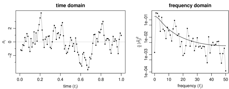
Figure 1: The example data $n_{i}$ in the time domain, and its (empirical) power $\frac{\Delta_{t}}{N}|\tilde{n}_{j}|^{2}$ in the Fourier domain. The solid line in the right panel shows the theoretical (2-sided) power spectral density in comparison.

As a simple example of non-white noise, the data are generated from an autoregressive process

$$n(t_{i})\;=\;\textstyle\frac{3}{4}n(t_{i-1})+x(t_{i}),$$ (43)

where the innovations $x(t_{i})$ are drawn independently from a uniform distribution across the interval $[-\sqrt{3},\sqrt{3}]$, so that they have zero mean and unit variance. The overall variance of the process defined in this way is $\mathrm{Var}\bigl{(}n(t_{i})\bigr{)}=2.29$; due to the positive correlation of subsequent samples it has a higher power at low frequencies and less at high frequencies. Figure 1 shows a noise sample generated using the above prescription, together with its theoretical power spectral density.

We will now apply the noise model introduced above and derive the posterior distribution of the noise parameters. Assuming one has a rough idea of the noise variance, we set the prior scale parameters $s^{2}_{j}$ so that the noise is a priori white with a prior expectation of $\mathrm{E}\bigl{[}\mathrm{Var}\bigl{(}n(t_{i})\bigr{)}\bigr{]}=2.50$. We use $\nu_{j}=3$ degrees of freedom, so that the noise parameters’ (and with that, the overall power’s) prior expectations are finite, while the variances are not. Prior scale and prior expectation then are $s^{2}_{j}=0.0166$, and $\mathrm{E}[\sigma_{j}^{2}]=0.05$.

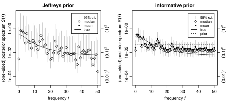
Figure 2: Posterior distributions of the 51 spectrum parameters $\sigma_{j}^{2}$ based on the data shown in figure 1. The left plot shows the posterior corresponding to the uninformative (and improper) Jeffreys prior. Posterior expectations do not exist in this case. The right plot corresponds to assuming a priori white noise with $\nu_{j}=3$ degrees of freedom for each frequency bin; the dashed line marks the prior expectation value.

Figure 2 illustrates the resulting posterior distribution for all 51 noise parameters (21) in comparison to the case of using the uninformative (and improper) Jeffreys prior. The Jeffreys prior (with $\nu_{j}=0$ degrees of freedom for each frequency bin) does not depend on the scale parameters $s_{j}^{2}$, and the resulting posterior with $\leq 2$ degrees of freedom at each frequency does not have finite expectation values. Note also that the posterior distributions corresponding to the first and last frequency bin (zero and Nyquist frequencies, $\sigma_{0}^{2}$ and $\sigma_{50}^{2}$) are wider than the others in both cases, as they have one less degree of freedom.

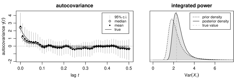
Figure 3: Posterior distributions of autocovariance and variance; the distributions shown here were derived via Monte Carlo integration.

Figure 3 shows the posterior distributions of autocovariance and variance, which are functions of the individual spectrum parameters $\sigma^{2}_{j}$. The variance may either be considered as the zero-lag autocovariance $\gamma(0)$ (see (2.3)), or as the integrated power $\mathcal{I}_{[0,f_{N/2}]}$ across the whole frequency range (see (8)).

3.2 A signal with additive noise

In the following example we will consider a time series where the primary interest is in a signal component, while the additive noise component will be modelled using the approach introduced above. As in the previous section, we will again consider $N=100$ data points $y(t_{1}),\ldots,y(t_{100})$ that are modelled as

$$y(t_{i})\;=\;g_{f,\dot{f},a,\phi}(t_{i})\,+\,n_{\vec{\sigma}}(t_{i}),$$ (44)

where $n_{\vec{\sigma}}(t_{i})$ is non-white noise of unknown spectrum, and $g_{f,\dot{f},a,\phi}(t)$ is a “chirping” signal waveform of increasing frequency:

$$g_{f,\dot{f},a,\phi}(t)\;=\;a\,\sin(2\pi(f+\dot{f}t)t+\phi)$$ (45)

where $f$ and $\dot{f}$ are the frequency and frequency derivative, $a$ is the amplitude, and $\phi$ is the phase. The noise again is generated the same way as in the previous example, by simulating an autoregressive process. The signal’s “size” relative to the noise is given by the signal-to-noise ratio (SNR: $\varrho=\sqrt{4\sum_{j}\frac{\frac{\Delta_{t}}{N}|\tilde{g}(f_{j})|^{2}}{S_{1}(f_{j})}}$), which here is at 15.

We define the signal parameters’ prior as uniform for phase, frequency and amplitude ($\phi\in[0,2\pi]$, $f\in[1,50]$ and $a\in[0,10]$) and normal for the frequency derivative $\dot{f}$ (zero mean and standard deviation 5). The prior distribution for the noise parameters $\sigma^{2}_{0},\ldots,\sigma^{2}_{50}$ is set exactly as in the previous section 3.2. For comparison, we analyze the data two more times, once assuming the true noise spectrum to be known, and once assuming the noise to be white, but with an unknown variance. In the latter case, we again assume a (conjugate) $\mbox{Inv-}\chi^{2}$ prior with an expectation of 2.5 and 3 degrees of freedom for the variance parameter.

The posterior distributions of signal and noise parameters may now be derived via Monte Carlo integration; we implemented a Metropolis sampler to simulate draws from the joint posterior probability distribution of all parameters [34]. For the model including the coloured noise spectrum as unknown, the signal parameters ($f$, $\dot{f}$, $a$, $\phi$) may be sampled based on the marginal likelihood expression (27), while samples of the 51 noise parameters ($\sigma^{2}_{0},\ldots,\sigma^{2}_{50}$) may then be sampled in an additional step via the conditional distribution of noise parameters for given signal parameters and the corresponding implied vector of noise residuals (21). Similarly, for the known spectrum model, sampling of the four signal parameters may be based on the likelihood expression (29), while sampling for the white noise model may be done using a Gibbs sampler alternately sampling from the conditional distributions of four signal parameters and the noise parameter [34].

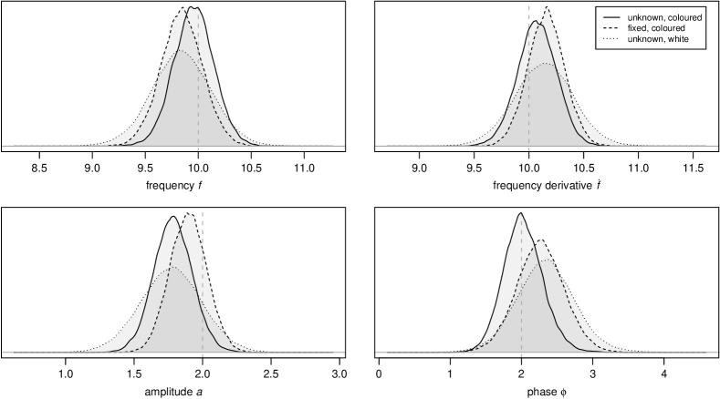
Figure 4: Marginal posterior densities of the four individual signal parameters. The three densities in each panel result from three different models applied for the noise term. The “unknown, coloured” case corresponds to the model introduced above, the “fixed, coloured” case assumes the true noise spectrum to be a priori known, and in the “unknown white” case the noise is modelled as white with unknown variance. The vertical dashed lines indicate the true parameter values.

Figure 4 shows the resulting marginal posterior distributions of the four signal parameters in comparison.

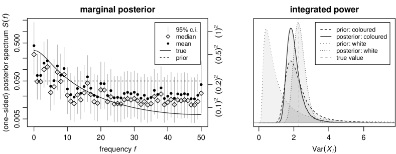
Figure 5: Marginal posterior distributions of the noise parameters. The left panel shows the posterior distribution for the 51 individual parameters of the coloured noise model. The right panel shows the prior and posterior distributions of the integrated power in comparison with the corresponding variance parameter in the white noise model.

One can see that application of the more flexible coloured noise model for the error term yields a more precise posterior distribution than the white noise model, and in fact the posterior is more similar to the case when the true noise spectrum is plugged into the model. Looking at the (marginal) posterior distributions of the noise parameters in figure 5, one can see that although the noise spectrum is only recovered with great uncertainty, this does not seem to harm the estimation of the signal parameters of actual interest. The overall variance is better recovered by the single-parameter white noise model, whereas the adaptability of the coloured noise model to the predominantly low-frequency noise (which is reflected in the posterior) seems to be the greater advantage. While the relative accuracy of the different methods is subject to a multitude of circumstances, one can see that depite its considerably greater complexity, the coloured noise model seems to perform competitively here.

4 Discussion

This work originated out of the Mock LISA Data Challenges (MLDC) [50], a gravitational wave parameter estimation effort in the context of the planned Laser Interferometer Space Antenna (LISA). Here parameters of a signal were to be inferred, where the signal was buried in noise known to be non-white and interspersed with a host of individual emission lines [17]. So the problem was to model a non-white, non-continuous spectrum where the shape of the spectrum was only vaguely known in advance [18, 19]. Also, the spectrum itself was not of primary interest, but rather a nuisance parameter that still needed to be accounted for along with the actual signal. Application of the method described here solved the problem and allowed the implementation of a Markov chain Monte Carlo (MCMC) algorithm based on a straightforward generalization of the commonly utilized Gaussian noise assumption, where modelling the spectrum complicated the analysis only slightly.

Several approaches to the simultaneous estimation of signal and noise parameters have been proposed before. An obvious way to model non-white noise would be to assume a particular time series formulation that allows for some flexibility in the resulting spectrum, for example an autoregressive (AR) model. Representations of this kind have been applied in various signal processing contexts, e.g. for detecting sinusoidal signals and estimating their parameters when these are buried in coloured noise [51, 52], or in the context of musical pitch estimation, where the signals to be modelled again are sinusoidal, but include higher harmonics and time-varying amplitudes [53]. If one is only interested in a narrow frequency band of the data, it may also be appropriate to model the noise spectrum as constant across the concerned range [54]. Regarding data treated in their Fourier domain representation, there is a rich literature concerned with the measurement of spectral densities (see e.g. [26] and references therein). However, there the aim is usually to produce consistent and smooth estimates of the spectrum, and the approaches applied include e.g. averaging [55, 32], smoothing via splines [56] or Bayesian model fitting [57, 58].

The approach to modelling the noise spectrum introduced here is different in that the spectrum per se is not of interest, or only of interest as far as it enters into likelihood computations. Smoothness or interpolation therefore are not primarily aimed for. What in fact is of concern is properly accounting for an a priori uncertainty in the (discretized, convolved) spectrum, in the frequency resolution that is given by the numerically Fourier transformed data, which then consequently entails the necessity for updating our knowledge about the spectrum as data is being processed. The resulting approach generalizes the model underlying the commonly used Whittle likelihood [29, 11, 30], and is hence essentially based on the “plain” periodogram of the noise time series, which for other purposes is commonly dismissed due to its unfavourable large-sample convergence behaviour. The model is very flexible as it is built upon a “binned” spectrum estimate without introducing any extra assumptions on the shape of the underlying noise spectral density. Its generality and simplicity make it useful for modelling residual noise at very little computational cost. In the way it is defined, the model is very general; it is a generalization of the model that constitutes the basis for matched filtering (e.g. [12, 13]) and that is commonly applied in signal processing problems (e.g. [11]), which then in turn constitutes the special case of an a priori known spectrum. The additional feature of the approach introduced here is that it allows to specify corresponding uncertainties in addition to the (prior) scale of the noise spectrum. Marginalization over the uncertainty in the noise spectrum yields a Student-$t$ model for the Fourier-domain data as a natural generalization of the common normal model. Due to the straightforward interpretability of the model and its computationally convenient form, we expect it to be particularly useful for modelling an unknown noise spectrum that constitutes a nuisance parameter rather than being of interest in itself. In that sense, the approach is not primarily aimed at gaining information about an unknown spectrum, but rather at properly accounting for uncertainty, and avoiding bias from supposedly precise a priori knowledge of the spectrum.

Alternatively, the Student-$t$ model may also be viewed as a generalized, robust model accommodating for heavier-tailed, non-Gaussian, or non-stationary noise. Related approaches are commonly used in many other applications in the context of robust statistics [37, 38, 39, 40, 43, 44]. In fact, the use of similar methods for accommodating noise outliers have already been advocated in the context of gravitational wave signal processing [41, 42]. Along similar lines, Clark et al. [59] implemented a (sine-Gaussian) noise-glitch component into the noise model. Principe and Pinto [60] suggested the use of a dictionary of glitch “atoms” in order to account for burst-like noise events. Veitch and Vecchio [61] implemented a coherence test based on a model selection procedure that is able to discriminate noise glitches (that appear independently in the data) from actual astrophysical events (that appear coherently in several data streams). Similarly, Littenberg and Cornish [62] extend their model to allow for excess noise that is isolated in time and frequency via a wavelet approach. Middleton [63] treated the general case of Gaussian noise with superimposed Poisson-distributed impulse noise bursts. We are planning to investigate the performance and sensitivity of a Student-$t$ model for robust detection and parameter estimation in real interferometer noise.

We expect the approach to be especially useful as a model component properly accounting for non-white residual noise, at little computational cost and without introducing overly restrictive assumptions about the noise. The interpretability of the Student-$t$ model in the context of robust modeling and M-estimation also makes it straightforwardly useful for robust inference. In that way, it may particularly be useful in signal processing contexts [64, 13], but it should be applicable in any case where a model for (residual) noise is needed [23, 65]. The fact that the model represents noise properties in terms of its power spectral density and is specified through physically meaningful parameters may make it particularly appealing in physical or engineering applications, where modelling is commonly based on Fourier-domain descriptions, and a time-domain formulation might be hard to incorporate or motivate. The advantage from application of the more flexible Student-$t$ model will very much depend on the particular inference problem at hand. The common normal model will obviously be optimal when its assumptions are met, and the degree to which one will outperform the other will depend on the particular departure(s) from Gaussianity, or on the imperfect prior knowledge of the spectrum, even if the data are perfectly Gaussian. While the range of possible deviations from the standard Gaussian model is infinite, some insight into the behaviour of a Student-$t$ model may be gained from the robust statistics literature; the properties of such an approach for location estimation has been investigated via Monte Carlo studies [66, 39] as well as theoretical considerations of key figures like relative efficiency or breakdown point [39, 43, 44]. A case study in the regression context may be found in [38].

The above basic model may in future be extended by introducing smoothness constraints on the spectrum. This might for example be approached by considering correlations between neighbouring spectral bins, or by assuming a piecewise constant spectrum, similar to what was done in [54]; the latter approach would in fact be a compromise between two models used in the example discussed above (Sec. 3.2), namely a flat spectrum and individually modelled frequency bins. Another interesting extension would be the incorporation of cross-spectra [23, 67]. Some of the methods described here have been coded as an R software extension package and are available for free download [68].

Appendix

A.1 Discrete Fourier transform (DFT)

The Fourier transform convention used in this paper is specified below; it is defined for a real-valued function $h$ of time $t$, sampled at $N$ discrete time points, at a sampling rate of $\frac{1}{\Delta_{t}}$, and it maps from

$$\{h(t)\in\mathds{R}:\;t=0,\Delta_{t},2\Delta_{t},\ldots,(N-1)\Delta_{t}\}$$ (46)

to a function of frequency $f$

$$\textstyle\{\tilde{h}(f)\in\mathds{C}:\;f=0,\Delta_{f},2\Delta_{f},\ldots,(N-1)\Delta_{f}\},$$ (47)

where $\Delta_{f}=\frac{1}{N\Delta_{t}}$ and

$$\tilde{h}(f)\;=\;\sum_{j=0}^{N-1}h(j\Delta_{t})\exp(-2\pi\mathrm{i}j\Delta_{t}f).$$ (48)

The inverse DFT then is given by

$$h(t)\;=\;\frac{1}{N}\sum_{j=0}^{N-1}\tilde{h}(j\Delta_{f})\exp(2\pi\mathrm{i}j\Delta_{f}t)$$ (49)

[22].

A.2 Relationship between DFT and time series model

Let

$$\alpha_{j}\;=\;\mathrm{Re}\bigl{(}\tilde{h}(f_{j})\bigr{)}\quad\mbox{and}\quad\beta_{j}\;=\;\mathrm{Im}\bigl{(}\tilde{h}(f_{j})\bigr{)},$$ (50)

i.e.: $\tilde{h}(f_{j})=\alpha_{j}+\beta_{j}\mathrm{i}$. For simplicity, in the following $N$ is assumed to be even; for uneven $N$ the derivation is similar. The inverse DFT was defined as (49):

$$h(t) = \frac{1}{N}\sum_{j=0}^{N-1}\tilde{h}(f_{j})\exp(2\pi\mathrm{i}f_{j}t)$$ (52)

$$= \frac{1}{N}\sum_{j=1}^{\frac{N}{2}-1}\Bigl{[}\bigl{(}2\alpha_{j}\cos(2\pi f_{j}t)+2(-\beta_{j})\sin(2\pi f_{j}t)\bigr{)}\Bigr{]}$$

$$+\,\textstyle\frac{1}{N}\alpha_{0}\,+\,\textstyle\frac{1}{N}\alpha_{N/2}\cos(2\pi\mathrm{i}f_{N/2}t)$$

where $t\in\{0,\Delta_{t},2\Delta_{t},\ldots,(N-1)\Delta_{t}\}$, and $f_{j}=j\Delta_{f}=\frac{j}{N\Delta_{t}}$ are the Fourier frequencies. So, comparing to (1), one can see that the realizations of $a_{0},\ldots,a_{\lfloor N/2\rfloor}$ and $b_{0},\ldots,b_{\lfloor N/2\rfloor}$ are derived from a given time series by Fourier-transforming and then setting

$$a_{j}\;=\;\textstyle\kappa_{j}\,\sqrt{\frac{\Delta_{t}}{N}}\,\alpha_{j}\quad\mbox{and}\quad b_{j}\;=\;\textstyle-\kappa_{j}\,\sqrt{\frac{\Delta_{t}}{N}}\,\beta_{j}$$ (53)

for $j=0,\ldots,\lfloor N/2\rfloor$, which especially implies that

$$a_{j}^{2}+b_{j}^{2}\;=\;\textstyle\kappa_{j}^{2}\,\frac{\Delta_{t}}{N}\,(\alpha_{j}^{2}+\beta_{j}^{2})\;=\;\textstyle\kappa_{j}^{2}\,\frac{\Delta_{t}}{N}\,\bigl{|}\tilde{h}(f_{j})\bigr{|}^{2}.$$ (54)

References

References

- [1] K. S. Thorne. Gravitational radiation. In S. W. Hawking and W. Israel, editors, 300 years of gravitation, chapter 9, pages 330–358. Cambridge University Press, Cambridge, 1987.
- [2] B. F. Schutz. Gravitational wave astronomy. Classical and Quantum Gravity, 16(12A):A131–A156, December 1999.
- [3] D. Sigg et al. Status of the LIGO detectors. Classical and Quantum Gravity, 25(11):114041, June 2008.
- [4] H. Grothe et al. The GEO 600 status. Classical and Quantum Gravity, 27(8):084003, April 2010.
- [5] T. Accadia et al. Commissioning status of the Virgo interferometer. Classical and Quantum Gravity, 27(8):084002, April 2010.
- [6] K. Arai et al. Status of Japanese gravitational wave detectors. Classical and Quantum Gravity, 26(20):204020, October 2009.
- [7] G. Harry et al. Advanced LIGO: the next generation of gravitational wave detectors. Classical and Quantum Gravity, 27(8):084006, April 2010.
- [8] K. Kuroda et al. Status of LCGT. Classical and Quantum Gravity, 27(8):084004, April 2010.
- [9] K. Danzmann and A. Rüdiger. LISA technology—concept, status, prospects. Classical and Quantum Gravity, 20(10):S1–S9, May 2003.
- [10] M. Punturo et al. The third generation of gravitational wave observatories and their science reach. Classical and Quantum Gravity, 27(8):084007, April 2010.
- [11] L. S. Finn. Detection, measurement, and gravitational radiation. Physical Review D, 46(12):5236–5249, December 1992.
- [12] G. L. Turin. An introduction to matched filters. IRE Transactions on Information Theory, 6(3):311–329, June 1960.
- [13] L. A. Wainstein and V. D. Zubakov. Extraction of signals from noise. Prentice-Hall, Englewood Cliffs, NJ, 1962.
- [14] C. Röver, R. Meyer, and N. Christensen. Coherent Bayesian inference on compact binary inspirals using a network of interferometric gravitational wave detectors. Physical Review D, 75(6):062004, March 2007.
- [15] A. C. Searle, P. J. Sutton, and M. Tinto. Bayesian detection of unmodeled bursts of gravitational waves. Classical and Quantum Gravity, 26(15):155017, August 2009.
- [16] P. Jaranowski and A. Królak. Gravitational-wave data analysis. Formalism and sample applications: The Gaussian case. Living Reviews in Relativity, 8(3), 2005. URL: http://www.livingreviews.org/lrr-2005-3.
- [17] L. Barack and C. Cutler. Confusion noise from LISA capture sources. Physical Review D, 70(12):122002, December 2004.
- [18] C. Röver. Bayesian inference on astrophysical binary inspirals based on gravitational-wave measurements. PhD thesis, The University of Auckland, 2007. URL: http://hdl.handle.net/2292/2356.
- [19] C. Röver, A. Stroeer, E. Bloomer, N. Christensen, J. Clark, M. Hendry, C. Messenger, R. Meyer, M. Pitkin, J. Toher, R. Umstätter, A. Vecchio, J. Veitch, and G. Woan. Inference on inspiral signals using LISA MLDC data. Classical and Quantum Gravity, 24(19):S521–S527, October 2007.
- [20] G. M. Jenkins. General considerations in the analysis of spectra. Technometrics, 3(2):167–190, May 1961.
- [21] E. T. Jaynes. Probability theory: The logic of science. Cambridge University Press, Cambridge, 2003.
- [22] P. C. Gregory. Bayesian logical data analysis for the physical sciences. Cambridge University Press, Cambridge, 2005.
- [23] G. M. Jenkins and D. G. Watts. Spectral analysis and its applications. Holden-Day, San Francisco, 1968.
- [24] G. L. Bretthorst. The near-irrelevance of sampling frequency distributions. In W. v. d. Linden et al., editors, Maximum Entropy and Bayesian Methods, pages 21–46. Kluwer Academic Publishers, Dordrecht, The Netherlands, 1999.
- [25] R. A. Fisher. Tests of significance in harmonic analysis. Proceedings of the Royal Society of London, Series A, 125(796):54–59, August 1929.
- [26] D. R. Brillinger. Time series: Data analysis and theory. McGraw-Hill, New York, 1981.
- [27] D. C. Champeney. A handbook of Fourier theorems. Cambridge University Press, 1987.
- [28] T. Kawata. On the Fourier series of a stationary stochastic process. Zeitschrift für Wahrscheinlichkeitstheorie und verwandte Gebiete, 6(3):224–245, September 1966.
- [29] P. Whittle. Curve and periodogram smoothing. Journal of the Royal Statistical Society B, 19(1):38–63, 1957.
- [30] N. Choudhuri, S. Ghosal, and A. Roy. Contiguity of the Whittle measure for a Gaussian time series. Biometrika, 91(4):211–218, 2004.
- [31] M. S. Taqqu. Weak stationarity. In S. Kotz and N. L. Johnson, editors, Encyclopedia of statistical sciences. Wiley & Sons, New York, 1988.
- [32] F. J. Harris. On the use of windows for harmonic analysis with the discrete Fourier transform. Proceedings of the IEEE, 66(1):51–83, January 1978.
- [33] A. M. Mood, F. A. Graybill, and D. C. Boes. Introduction to the theory of statistics. McGraw-Hill, New York, 3rd edition, 1974.
- [34] A. Gelman, J. B. Carlin, H. Stern, and D. B. Rubin. Bayesian data analysis. Chapman & Hall / CRC, Boca Raton, 1997.
- [35] H. Jeffreys. An invariant form for the prior probability in estimation problems. Proceedings of the Royal Society of London, Series A, 186(1007):453–461, September 1946.
- [36] W. M. Bolstad. Introduction to Bayesian Statistics, chapter 15, pages 297–316. Wiley, 2nd edition, 2007.
- [37] K. L. Lange, R. J. A. Little, and J. M. G Taylor. Robust statistical modeling using the distribution. Journal of the American Statistical Association, 84(408):881–896, December 1989.
- [38] J. Geweke. Bayesian treatment of the independent Student- linear model. Journal of Applied Econometrics, 8:S19–S40, December 1993.
- [39] D. R. Divgi. Robust estimation using Student’s distribution. CNA Research Memorandum CRM 90-217, Center for Naval Analyses, Alexandria, VA, USA, December 1990.
- [40] J. B. McDonald and W. K. Newey. Partially adaptive estimation of regression models via the generalized distribution. Econometric Theory, 4(3):428–457, December 1988.
- [41] J. D. Creighton. Data analysis strategies for the detection of gravitational waves in non-Gaussian noise. Physical Review D, 60(2):021101, July 1999.
- [42] B. Allen, J. D. E. Creighton, É. É. Flanagan, and J. D. Romano. Robust statistics for deterministic and stochastic gravitational waves in non-Gaussian noise: Frequentist analyses. Physical Review D, 65(12):122002, June 2002.
- [43] F. R. Hampel, E. M. Ronchetti, P. J. Rousseeuw, and W. A. Stahel. Robust statistics: The approach based on influence functions. Wiley, New York, 1986.
- [44] P. J. Huber and E. M. Ronchetti. Robust statistics. Wiley, 2nd edition, 2009.
- [45] H. H. Kelejian and I. R. Prucha. Independent or uncorrelated disturbances in linear regression: An illustration of the difference. Economics Letters, 19(1):35–38, 1985.
- [46] T. S. Breusch, J. C. Robertson, and A. H. Welsh. The emperor’s new clothes: a critique of the multivariate regression model. Statistica Neerlandica, 51(3):269–286, December 2001.
- [47] T. Mäkeläinen, K. Schmidt, and G. P. H. Styan. On the existence and uniqueness of the maximum likelihood estimate of a vector-valued parameter in fixed-size samples. The Annals of Statistics, 9(4):758–767, July 1981.
- [48] B. C. Sutradhar and M. M. Ali. Estimation of the parameters of a regression model with a multivariate error variable. Communications in Statistics - Theory and Methods, 15(2):429–450, 1986.
- [49] R. S. Singh. Estimation of error variance in linear regression models with errors having multivariate Student- distribution with unknown degrees of freedom. Economics Letters, 27(1):47–53, 1988.
- [50] K. A. Arnaud et al. An overview of the Mock LISA Data Challenges. In S. M. Merkowitz and J. C. Livas, editors, Laser Interferometer Space Antenna: 6th International LISA Symposium, volume 873 of AIP conference proceedings, pages 619–624, November 2006.
- [51] C. Chatterjee, R. L. Kashyap, and G. Boray. Estimation of close sinusoids in colored noise and model discrimination. IEEE Transactions on Acoustics, Speech, and Signal Processing, ASSP-35(3):328–337, March 1987.
- [52] C.-M. Cho and P. M. Djurić. Bayesian detection and estimation of cisoids in colored noise. IEEE Transactions on Signal Processing, 43(12):2943–2952, December 1995.
- [53] S. Godsill and M. Davy. Bayesian harmonic models for musical pitch estimation and analysis. In Proceedings of the IEEE international conference on acoustics, speech and signal processing (ICASSP) 2002, volume 2, pages 1769–1772. IEEE, 2002.
- [54] R. J. Dupuis and G. Woan. Bayesian estimation of pulsar parameters from gravitational wave data. Physical Review D, 72(10):102002, November 2005.
- [55] P. D. Welch. The use of Fast Fourier Transform for the estimation of power spectra: A method based on time averaging over short, modified periodograms. IEEE Transactions on Audio and Electroacoustics, AU-15(2):70–73, June 1967.
- [56] G. Wahba. Automatic smoothing of the log periodogram. Journal of the American Statistical Association, 75(369):122–132, March 1980.
- [57] A. K. Gangopadhyay, B. K. Mallik, and D. G. T. Denison. Estimation of spectral density of a stationary time series via an asymptotic representation of the periodogram. Journal of Statistical Planning and Inference, 75(2):281–290, January 1999.
- [58] N. Choudhuri, S. Ghosal, and A. Roy. Bayesian estimation of the spectral density of a time series. Journal of the American Statistical Association, 99(468):1050–1059, December 2004.
- [59] J. Clark, I. S. Heng, M. Pitkin, and G. Woan. Evidence-based search method for gravitational waves from neutron star ring-downs. Physical Review D, 76(4):043003, August 2007.
- [60] M. Principe and I. M. Pinto. Locally optimum network detection of unmodelled gravitational wave bursts in an impulsive noise background. Classical and Quantum Gravity, 26(4):045003, February 2009.
- [61] J. Veitch and A. Vecchio. Bayesian coherent analysis of in-spiral gravitational wave signals with a detector network. Physical Review D, 81(6):062003, March 2010.
- [62] T. Littenberg and N. Cornish. Separating gravitational wave signals from instrument artifacts. Arxiv preprint 1008.1577, August 2010.
- [63] D. Middleton. On the theory of random noise. Phenomenological models. Journal of Applied Physics, 22:1143–1163, 1326, 1951.
- [64] R. N. McDonough and A. D. Whalen. Detection of signals in noise. Academic Press, New York, 2nd edition, 1995.
- [65] P. Bloomfield. Fourier analysis of time series: An introduction. Wiley & Sons, New York, 2nd edition, 2000.
- [66] D. F. Andrews et al. Robust estimates of location: survey and advances. Princeton University Press, Princeton, NJ, USA, 1972.
- [67] M. Nofrarias, C. Röver, M. Hewitson, A. Monsky, G. Heinzel, K. Danzmann, L. Ferraioli, M. Hueller, and S. Vitale. Bayesian parameter estimation in the second LISA Pathfinder Mock Data Challenge. Arxiv preprint 1008.5280 [gr-qc], August 2010.
- [68] C. Röver. bspec: Bayesian spectral inference, 2008. R package. URL: http://cran.r-project.org/package=bspec.