Can electro-magnetic field, anisotropic source and varying $\Lambda$ be sufficient to produce wormhole spacetime ?

Abstract

It is well known that solutions of general relativity which allow for traversable wormholes require the existence of exotic matter ( matter that violates weak or null energy conditions [WEC or NEC] ). In this article, we provide a class of exact solution for Einstein-Maxwell field equations describing wormholes assuming the erstwhile cosmological term $\Lambda$ to be space variable , viz., $\Lambda=\Lambda(r)$. The source considered here not only a matter entirely but a sum of matters i.e. anisotropic matter distribution, electromagnetic field and cosmological constant whose effective parts obey all energy conditions out side the wormhole throat. Here violation of energy conditions can be compensated by varying cosmological constant. The important feature of this article is that one can get wormhole structure, at least theoretically, comprising with physically acceptable matters.

Introduction:

We know a wormhole is a hypothetical topological feature of spacetime that connects two distinct spacetimes. The wormhole idea comes from Einstein’s theory of general relativity [1]. It is the solution of Einstein equation shared by the violation of null energy condition. The matter that characterized above stress energy tensor is known as exotic matter. Needless to say, the notion of this exotic matter is bizarre. In spite of, several physicists have constructed wormholes by assuming different forms of exotic matter. Sushkov[2], Lobo[3], Kuhfittig[4], Zaslovskii[5], Rahaman et al[6] have presented wormhole solutions comprising of phantom energy. Lobo [7] , Rahaman et al [7] and Rashid et al [7] have shown that wormholes may be supported by the Chaplygin gas. Das et al[8] have studied wormhole with Tachyonic field. Mansouryar[9] and Khabibullin A et al [10] have assumed Casimir field for exotic matter source. Rahaman et al [11] have studied wormhole in presence of C-field. Also Rahaman et al [12] have shown that wormholes may exist in Kalb-Ramond spacetime.

To avoid this bizarre form of matter distribution, several authors used scalar tensor theory of gravity to construct wormholes[13]. Though Visser et al[14] showed and latter supported by Kuhffitig[15], Nandi et al[16] and Fewster et al[17] that the amount of exotic matter needed can be made arbitrarily small for constructing wormholes but no matter how difficult to deal with exotic matter. So we are trying to provide a prescription how to get a wormhole comprising with physically acceptable matters. We give a class of solution of Einstein-Maxwell field equations describing wormholes assuming cosmological term $\Lambda$ to be space variable. The source considered here not only a matter entirely but a sum of matters i.e. anisotropic matter distribution, electromagnetic field and cosmological constant whose effective parts obey all energy conditions out side the wormhole throat. Here violation of energy conditions can be compensated by varying cosmological constant. The assumption of variable $\Lambda$ is not new [ see ref.[18], for review ]. Several authors have discussed the contribution of space dependence $\Lambda$ to the effective gravitational mass of the astrophysical systems[19]. The solutions of Einstein field equations with variable $\Lambda$ have a wider range of application to discuss more accurately the local massive objects like galaxies[20] and energy density of classical electron[21]. So, it is not unnatural to inclusion of $\Lambda$ on an anisotropic static spherically symmetric source to construct wormholes. Recently Lemos et al [22] have studied extensively wormhole geometry in presence of $\Lambda$ where $\Lambda$ is a constant. The aim of the present investigation is to construct stable traversable wormhole with realistic matter sources.

Basic equations for constructing wormholes:

Let us consider a static, spherically symmetric matter distribution corresponding to the line element

$$ds^{2}=-e^{\nu(r)}dt^{2}+e^{\mu(r)}dr^{2}+r^{2}(d\theta^{2}+sin^{2}\theta d\phi^{2})$$ (1)

The Einstein-Maxwell field equations for the above spherically symmetric metric corresponding to the charged anisotropic matter distribution in presence of varying $\Lambda$ are given by

$$e^{-\mu}[\frac{\mu^{\prime}}{r}-\frac{1}{r^{2}}]+\frac{1}{r^{2}}=8\pi\rho+E^{2}+\Lambda$$ (2)

$$e^{-\mu}[\frac{1}{r^{2}}+\frac{\nu^{\prime}}{r}]-\frac{1}{r^{2}}=8\pi p_{r}-E^{2}-\Lambda$$ (3)

$$\frac{1}{2}e^{-\mu}[\frac{1}{2}(\nu^{\prime})^{2}+\nu^{\prime\prime}-\frac{1}{2}\mu^{\prime}\nu^{\prime}+\frac{1}{r}({\nu^{\prime}-\mu^{\prime}})]=8\pi p_{t}+E^{2}-\Lambda$$ (4)

and

$$(r^{2}E)^{\prime}=4\pi r^{2}\sigma e^{\frac{\mu}{2}}$$ (5)

Equation (5) can equivalently be expressed in the form

$$E(r)=\frac{1}{r^{2}}\int_{0}^{r}4\pi r^{2}\sigma e^{\frac{\mu}{2}}dr=\frac{q(r)}{r^{2}}$$ (6)

where $q(r)$ is the total charge of the sphere under consideration. Also, the conservation equation is given by

$$\frac{d}{dr}(p_{r}-\frac{\Lambda}{8\pi})+(\rho+p_{r})\frac{\nu^{\prime}}{2}=\frac{1}{8\pi r^{4}}\frac{dq^{2}}{dr}+\frac{2(p_{t}-p_{r})}{r}$$ (7)

Here, $\rho,p_{r},p_{t},E,\sigma$ and $q$ are respectively the matter energy density, radial and tangential pressures, electric field strength, electric charged density and electric charge. The prime denotes derivative with respect to ’r’.



Solutions:

Now to get exact solutions, we assume the following assumptions:

(a)

$$\nu(r)=0$$ (8)

Argument: One of the traversability properties is the tidal gravitational forces experienced by a traveller must be reasonably small. So, we assume a zero tidal force as seen by the stationary observer. Thus one of the traversability conditions is automatically satisfied.

(b)

$$p_{t}=np_{r}$$ (9)

Argument: Pressures are anisotropic with $p_{t}<p_{r}$.

(c)

$$p_{r}=m\rho$$ (10)

Argument: The above equation indicates the equation of state with $0<m<1$.

(d) $\frac{\Lambda}{8\pi}\propto p_{r}$

i.e.

$$\frac{\Lambda}{8\pi}=ap_{r}$$ (11)

( $a$ is proportional constant )

Argument: The vacuum energy ( which is equivalent to $\Lambda$ ) can be thought as a contribution of the energy stress components.

(e)

$$\sigma e^{\frac{\mu}{2}}=\sigma_{0}r^{s}$$ (12)

( $\sigma_{0}$ and s are arbitrary constants )

Argument: In usual sense, the term $\sigma e^{\frac{\mu}{2}}$ occurring inside the integral sign in the equation (6), is called the volume charge density and hence the condition $\sigma e^{\frac{\mu}{2}}=\sigma_{0}r^{s}$ , can equivalently be interpreted as the volume charge density being polynomial function of ’r’. The constant $\sigma_{0}$ is the charge density at $r=0$, the center of the charged matter [19].

Taking into account of equations (8) - (12), one gets the following solutions of the field equations (2) - (7) as

$$q^{2}(r)=\frac{16\pi^{2}\sigma_{0}^{2}}{(s+3)^{2}}r^{2s+6}$$ (13)

$$E^{2}(r)=\frac{16\pi^{2}\sigma_{0}^{2}}{(s+3)^{2}}r^{2s+2}$$ (14)

$$p_{r}=Dr^{\frac{-2(1-n)}{(1-a)}}+\frac{4\pi\sigma_{0}^{2}}{P}r^{2s+2}$$ (15)

where $P=(s+3)[2(1-n)+(2s+2)(1-a)]$ and D is an integration constant.

$$e^{-\mu}=1-\frac{b(r)}{r}$$ (16)

where,

$$b(r)=Fr^{\frac{(2n+1-3a)}{(1-a)}}+Xr^{2s+5}$$ (17)

where, $F=\frac{8\pi D(1-a)(a+\frac{1}{m})}{(2n+1-3a)}$

and

$X=\frac{16\pi^{2}\sigma_{0}^{2}}{(2s+5)}[\frac{1}{(s+3)^{2}}+\frac{(a+\frac{1}{m})}{P}]$

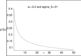
Figure 1: Electric charge with respect to radial coordinate ’r’.

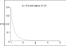
Figure 2: Electric field strength with respect to radial coordinate ’r’.

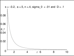
Figure 3: Radial pressure with respect to radial coordinate ’r’.

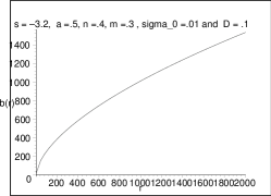
Figure 4: Shape function with respect to radial coordinate ’r’.

Properties of the solutions: Since the space time is asymptotically flat i.e. $\frac{b(r)}{r}\rightarrow 0$ as $r\rightarrow\infty$, the Eq.(17) is consistent only when $\frac{(2n+1-3a)}{(1-a)}-1<0$ and $2s+4<0$.

These imply,

$$n<a$$ (18)

and

$$s<-2$$ (19)

Also, as $\mid r\mid\rightarrow\infty$, $p_{r}$, $q^{2}(r)$ and $E^{2}(r)$ $\rightarrow 0$, so one has to take the following restriction on ’s’ as

$$s<-3$$ (20)

Here the throat occurs at $r=r_{0}$ for which $b(r_{0})=r_{0}$ i.e. $1=Fr_{0}^{\frac{(2(n-1)}{(1-a)}}+Xr_{0}^{2s+4}$. For the suitable choices of the parameters, the graph of the function $G(r)=b(r)-r$ indicates the point $r_{0}$ , where G(r) cuts the ’r’ axis (see fig. 5 ). From the graph, one can also note that when $r>r_{0}$, $G(r)<0$ i.e. $b(r)-r<0$. This implies $\frac{b(r)}{r}<1$ when $r>r_{0}$.

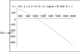
Figure 5: Throat occurs where $G(r)$ cuts ’r’ axis

Thus our solution describing a static spherically symmetric wormhole supported by anisotropic matter distribution in presence of electromagnetic field and varying $\Lambda$.

Stability :

To study the stability, we match our interior wormhole solution to the exterior Reissner-Nordström Black hole solution

$ds^{2}=-(1-\frac{2M}{r}+\frac{Q^{2}}{r^{2}})dt^{2}+\frac{dr^{2}}{(1-\frac{2M}{r}+\frac{Q}{r^{2}})}+r^{2}d\Omega_{2}^{2},$

at the junction interface S, situated outside the event horizon, $a>r_{h}=M\pm\sqrt{M^{2}-Q^{2}}$, one needs to use extrinsic curvature or second fundamental forms associated with two sides of the shell ’S’ as $K_{ij}^{\pm}=-n^{\pm}_{\mu;\nu}e^{\mu}_{(i)}e^{\nu}_{(j)}$, where $n^{\pm}$ are the unit normals to S and $e^{\mu}_{(i)}$ are the components of the holonomic basis vectors tangent to S. Using the Darmois-Israel formalism, we write Lanczos equations for the surface stress energy tensors $S_{j}^{i}$ at the junction interface S as

$$S_{j}^{i}=-\frac{1}{8\pi}([K_{j}^{i}]-\delta_{j}^{i}K)$$ (21)

where $S_{j}^{i}=diag(-\sigma,p_{\theta},p_{\phi})$ is the surface energy tensor with $\sigma$ , the surface density and $p_{\theta}$ and $p_{\phi}$, the surface pressures and $[K_{ij}]=K_{ij}^{+}-K_{ij}^{-}$ and $K=[K_{i}^{i}]=trace[K_{ij}]$.

To analyze the dynamics of the wormhole, we permit the radius of the throat to become a function of time, $a\rightarrow a(\tau)$. Now taking into account equation (21), one can find,

$$\sigma=-\frac{1}{4\pi a}[\sqrt{1-\frac{2M}{a}+\frac{Q^{2}}{a^{2}}+\dot{a}^{2}}-\sqrt{1-Fa^{u}-Xa^{w}+\dot{a}^{2}}]$$ (22)

$p_{\theta}=p_{\phi}=p=\frac{1}{8\pi a}\frac{1-\frac{M}{a}+a\ddot{a}+\dot{a}^{2}}{\sqrt{1-\frac{2M}{a}+\frac{Q^{2}}{a^{2}}+\dot{a}^{2}}}\\ -\frac{(1-Fa^{u}-Xa^{w}+\dot{a}^{2})+a\ddot{a}+\frac{\dot{a}^{2}(Fua^{u}+Xwa^{w})}{2(1-Fa^{u}-Xa^{w})}}{\sqrt{1-Fa^{u}-Xa^{w}+\dot{a}^{2}}}$

(23)

[ over dot means the derivatives with respect to $\tau$ and $u=\frac{2(n-a)}{(1-n)}$ ; $w=2s+4$ ]

Using conservation identity
$S^{i}_{j;i}=-[\dot{\sigma}+2\frac{\dot{a}}{a}(p+\sigma)]$ , one can get the following expression as

$${\sigma^{\prime}}=-\frac{2}{a}(p+\sigma)+Y$$ (24)

where,

$Y=-\frac{1}{4\pi a^{2}}[\frac{(Fua^{u}+Xwa^{w})}{2(1-Fa^{u}-Xa^{w})}\times\\ \sqrt{1-Fa^{u}-Xa^{w}+\dot{a}^{2}}]$

(25)

Rearranging equation (22), we obtain the thin shell’s equation of motion

$$\dot{a}^{2}+V(a)=0$$ (26)

Here the potential is defined as

$$V(a)=\frac{1}{2}(f_{1}+f_{2})-4\pi^{2}a^{2}\sigma^{2}-\frac{(f_{1}-f_{2})^{2}}{64\pi^{2}a^{2}\sigma^{2}}$$ (27)

where,

$$f_{1}=1-\frac{2M}{a}+\frac{Q^{2}}{a^{2}};f_{2}=1-Fa^{u}-Xa^{w}$$ (28)

Linearizing around a static solution situated at $a_{0}$, one can expand V(a) around $a_{0}$ to yield

$V=V(a_{0})+V^{\prime}(a_{0})(a-a_{0})+\frac{1}{2}V^{\prime\prime}(a_{0})(a-a_{0})^{2}\\ +0[(a-a_{0})^{3}]$

(29)

where prime denotes derivative with respect to $a$.

Since we are linearizing around a static solution at $a=a_{0}$, we have $V(a_{0})=0$ and $V^{\prime}(a_{0})=0$. The stable equilibrium configurations correspond to the condition $V^{\prime\prime}(a_{0})>0$.
Now we define a parameter $\beta$, which is interpreted as the speed of sound, by the relation

$$\beta^{2}(\sigma)=\frac{\partial p}{\partial\sigma}|_{\sigma}$$ (30)

Using equation (24), we have

$$\beta^{2}(\sigma)=-1+\frac{a}{2\sigma^{\prime}}[\frac{2}{a^{2}}(p+\sigma)+Y^{\prime}-\sigma^{\prime\prime}]$$ (31)

The wormhole solution is stable if $V^{\prime\prime}(a_{0})>0$ i.e.

$\frac{4\sigma^{\prime}}{a^{3}}[\frac{(f_{1}-f_{2})^{2}}{32\pi^{2}\sigma^{3}a^{2}}-8\pi^{2}\sigma a^{2}](1+\beta_{0}^{2})<\frac{1}{2}(f_{1}^{\prime\prime}+f_{2}^{\prime\prime})-8\pi^{2}(\sigma^{2}-4a\sigma\sigma^{\prime}-2a^{2}\sigma^{\prime 2})\linebreak+\frac{2}{a^{2}}[(p+\sigma)+Y^{\prime}][\frac{(f_{1}-f_{2})^{2}}{32\pi^{2}\sigma^{3}a^{2}}-8\pi^{2}\sigma a^{2}]-\frac{(f_{1}^{\prime}-f_{2}^{\prime})^{2}}{32\pi^{2}\sigma^{2}a^{2}}-\frac{(f_{1}-f_{2})(f_{1}^{\prime\prime}-f_{2}^{\prime\prime})}{32\pi^{2}\sigma^{2}a^{2}}\linebreak+\frac{(f_{1}-f_{2})(f_{1}^{\prime}-f_{2}^{\prime})}{16\pi^{2}\sigma^{2}a^{2}}(\frac{\sigma^{\prime}}{\sigma}+\frac{\sigma^{\prime}}{a}+\frac{2}{a})-\frac{(f_{1}-f_{2})^{2}}{16\pi^{2}\sigma^{2}a^{2}}(\frac{2\sigma^{\prime}}{a\sigma}+\frac{3}{2}(\frac{\sigma^{\prime}}{\sigma})^{2}+\frac{3}{2a^{2}})$

or,

$$\beta_{0}^{2}<\frac{A-B+C-S-T+G-H}{N-L}-1$$ (32)

where A, B, C, S, T, G, H, N, L are given in the appendix at $a=a_{0}$.

Thus if one treats $a_{0}$, M and Q and other parameters are specified quantities, then the stability of the configuration requires the above restriction on the parameter $\beta_{0}$. This means there exists some part of the parameter space where the throat location is stable. [ To get geometrical information, one can show the stability region graphically by plotting $\beta_{\mid(a=a_{0})}$ vs. $x=\frac{M}{a_{0}}$ and taking all other parameters as known quantities. The stability region is given below the curve. ]

Traversability conditions:

Now we will focus on the usability of our wormhole structure i.e. to check whether it is useful for the travellers of modern civilizations. To travel through a wormhole, the tidal gravitational forces experienced by a traveller must be reasonably small. According to Morris and Thorne [1], the acceleration felt by the traveller should not exceed Earth’s gravity. Thus the tidal accelerations between two parts of the traveller’s body, separated by say, 2 meters, must less than the gravitational acceleration at Earth’s surface $g_{earth}$ ( $g_{earth}\approx 10m/sec^{2}$ ). Due to Morris and Thorne [1], the testing tangential tidal constraint is given by ( assuming $\nu^{\prime}=0$ )

$|R_{t\theta t\theta}|=R_{t\phi t\phi}|=|\frac{\beta^{2}}{2r^{2}}(\frac{v}{c})^{2}(b^{\prime}-\frac{b}{r})|\leq\frac{g_{earth}}{2c^{2}m}\approx\frac{1}{10^{10}m^{2}}$

with $\beta=\frac{1}{\sqrt{1-(\frac{v}{c})^{2}}}$ and c is the velocity of light.

[ The above inequality indicates a restriction on traveller’s velocity $v(r)$ with which the traveller crosses the wormhole ]

For $v<<c$, we have $\beta\approx 1$ and substituting the expression of $b(r)$, we get

$\frac{v}{c}<\frac{1}{10^{8}}\sqrt{\frac{1}{\frac{Fu}{2}r^{u-2}+\frac{Xw}{2}r^{w-2}}}$

The above inequality represents the tangential tidal force and restrict the speed v of the while crossing the wormhole. Here radial acceleration is zero since $R_{rtrt}=0$, for our wormhole spacetime. Acceleration felt by a traveller should less than the gravitational acceleration at earth surface, $g_{earth}$. The condition imposed by Morris and Thorne [1] as

$|\textbf{f}|=|\sqrt{[1-\frac{b(r)}{r}}]\beta^{\prime}c^{2}|\leq g_{earth}$ [ for $\nu^{\prime}=0$]

For the traveller’s velocity $v=constant$, one finds that $|\textbf{f}|=0$. In our model the the above condition is automatically satisfied, the traveller feels a zero gravitational acceleration.

Final Remarks:

Our aim in this article is to search reasonable matters that produce wormhole like spacetime. We have been able to show that if we are supplied anisotropic matter source and electromagnetic field along with varying $\Lambda$, then one could construct, at least theoretically, a stable traversable wormhole. One can note that $\rho_{effective}>0,$ $\rho_{effective}$ + $p_{r}$ ${}_{effective}>0$, $\rho_{effective}$ + $p_{t}$ ${}_{effective}>0$ for all $r>r_{0}$ i.e. all energy conditions are satisfied out side the throat. But at the throat i.e. at $r=r_{0}$, NEC is violated. Nevertheless this wormhole has been constructed nearly accessible matter sources.

The collections of anisotropic matter and electromagnetic field are not difficult. The only difficult task is to collect the source ’$\Lambda$’. According to Zeldovich[23], $\Lambda$ is nothing but the vacuum energy density due to quantum fluctuations. If an engineer imbued with new ideas will able to produce vacuum energy density by means of quantum fluctuations, we imagine that wormhole could be constructed physically.

Acknowledgments

F.R is thankful to Jadavpur University and DST , Government of India for providing financial support. MK has been partially supported by UGC, Government of India under MRP scheme.

Appendix :

$A=\frac{1}{2}(f_{1}^{\prime\prime}+f_{2}^{\prime\prime})=\frac{1}{2}[\frac{6Q^{2}}{a^{4}}-\frac{4M}{a^{3}}-Fu(u-1)a^{u-2}-Xw(w-1)a^{w-2}]$

$B=8\pi^{2}(\sigma^{2}-4a\sigma\sigma^{\prime}-2a^{2}\sigma^{\prime 2})=\frac{1}{2a^{2}}(\sqrt{1-\frac{2M}{a}+\frac{Q^{2}}{a^{2}}}-\sqrt{1-Fa^{u}-Xa^{w}})^{2}+\frac{2}{a^{2}}(\sqrt{1-\frac{2M}{a}+\frac{Q^{2}}{a^{2}}}-\sqrt{1-Fa^{u}-Xa^{w}})(\frac{1-\frac{3M}{a}+\frac{2Q^{2}}{a^{2}}}{\sqrt{1-\frac{2M}{a}+\frac{Q^{2}}{a^{2}}}}-\frac{1-Fa^{u}-Xa^{w}+\frac{1}{2}Fua^{u}+\frac{1}{2}Xwa^{w}}{\sqrt{1-Fa^{u}-Xa^{w}}})-\frac{1}{a^{2}}(\frac{1-\frac{3M}{a}+\frac{2Q^{2}}{a^{2}}}{\sqrt{1-\frac{2M}{a}+\frac{Q^{2}}{a^{2}}}}-\frac{1-Fa^{u}-Xa^{w}+\frac{1}{2}Fua^{u}+\frac{1}{2}Xwa^{w}}{\sqrt{1-Fa^{u}-Xa^{w}}})^{2}$

$S=\frac{(f_{1}^{\prime}-f_{2}^{\prime})^{2}}{32\pi^{2}\sigma^{2}a^{2}}=\frac{1}{2}\frac{(Fua^{u-1}+Xwa^{w-1}+\frac{2M}{a^{2}}-\frac{2Q^{2}}{a^{3}})^{2}}{(\sqrt{1-\frac{2M}{a}+\frac{Q^{2}}{a^{2}}}-\sqrt{1-Fa^{u}-Xa^{w}})^{2}}$

$T=\frac{(f_{1}-f_{2})(f_{1}^{\prime\prime}-f_{2}^{\prime\prime})}{32\pi^{2}\sigma^{2}a^{2}}=\frac{1}{2}\frac{(Fa^{u}+Xa^{w}-\frac{2M}{a}+\frac{Q^{2}}{a^{2}})[Fu(u-1)a^{u-2}+Xw(w-1)a^{w-2}-\frac{4M}{a^{3}}+\frac{6Q^{2}}{a^{4}}]}{[\sqrt{1-\frac{2M}{a}+\frac{Q^{2}}{a^{2}}}-\sqrt{1-Fa^{u}-Xa^{w}}]^{2}}$

$G=\frac{(f_{1}-f_{2})(f_{1}^{\prime}-f_{2}^{\prime})}{16\pi^{2}\sigma^{2}a^{2}}[\frac{\sigma^{\prime}}{\sigma}+\frac{\sigma^{\prime}}{a}+\frac{2}{a}]=\frac{(Fa^{u}+Xa^{w}-\frac{2M}{a}+\frac{Q^{2}}{a^{2}})(Fua^{u-1}+Xwa^{w-1}+\frac{2M}{a^{2}}-\frac{2Q^{2}}{a^{3}})}{(\sqrt{1-\frac{2M}{a}+\frac{Q^{2}}{a^{2}}}-\sqrt{1-Fa^{u}-Xa^{w}})^{2}}\linebreak-\frac{1}{a}\frac{1}{(\sqrt{1-\frac{2M}{a}+\frac{Q^{2}}{a^{2}}}-\sqrt{1-Fa^{u}-Xa^{w}})}[(\frac{1-\frac{3M}{a}+\frac{2Q^{2}}{a^{2}}}{\sqrt{1-\frac{2M}{a}+\frac{Q^{2}}{a^{2}}}}-\frac{1-Fa^{u}-Xa^{w}+\frac{1}{2}Fua^{u}+\frac{1}{2}Xwa^{w}}{\sqrt{1-Fa^{u}-Xa^{w}}})+\frac{1}{4\pi a^{3}}(\frac{1-\frac{3M}{a}+\frac{2Q^{2}}{a^{2}}}{\sqrt{1-\frac{2M}{a}+\frac{Q^{2}}{a^{2}}}}-\frac{1-Fa^{u}-Xa^{w}+\frac{1}{2}Fua^{u}+\frac{1}{2}Xwa^{w}}{\sqrt{1-Fa^{u}-Xa^{w}}})+\frac{2}{a}]$ $C=\frac{2}{a^{2}}[(p+\sigma)+Y^{\prime}][\frac{(f_{1}-f_{2})^{2}}{32\pi^{2}\sigma^{3}a^{2}}-8\pi^{2}\sigma a^{2}]\linebreak=[\frac{1}{8\pi a}(\sqrt{1-Fa^{u}-Xa^{w}}-\frac{1-\frac{3M}{a}+\frac{2Q^{2}}{a^{2}}}{\sqrt{1-\frac{2M}{a}+\frac{Q^{2}}{a^{2}}}})+\frac{1}{4\pi a^{3}}(\frac{Fua^{u}+Xwa^{w}}{\sqrt{1-Fa^{u}-Xa^{w}}})]-\frac{1}{8\pi a^{2}}[\frac{\sqrt{1-Fa^{u}-Xa^{w}}(Fu^{2}a^{u-1}+Xw^{2}a^{w-1})+\frac{(Fua^{u}+Xwa^{w})(Fua^{u-1}+Xwa^{w-1})}{2\sqrt{1-Fa^{u}-Xa^{w}}}}{1-Fa^{u}-Xa^{w}}]\linebreak\times[\frac{4\pi}{a}[(\sqrt{1-\frac{2M}{a}+\frac{Q^{2}}{a^{2}}}-\sqrt{1-Fa^{u}-Xa^{w}})-\frac{(Fa^{u}+Xa^{w}-\frac{2M}{a}+\frac{Q^{2}}{a^{2}})^{2}}{(\sqrt{1-\frac{2M}{a}+\frac{Q^{2}}{a^{2}}}-\sqrt{1-Fa^{u}-Xa^{w}})^{3}}]]$

$H=\frac{(f_{1}-f_{2})^{2}}{16\pi^{2}\sigma^{2}a^{2}}[\frac{2\sigma^{\prime}}{a\sigma}+\frac{{3\sigma^{\prime}}^{2}}{2\sigma^{2}}+\frac{3}{2a^{2}}]=\frac{(Fa^{u}+Xa^{w}-\frac{2M}{a}+\frac{Q^{2}}{a^{2}})^{2}}{(\sqrt{1-\frac{2M}{a}+\frac{Q^{2}}{a^{2}}}-\sqrt{1-Fa^{u}-Xa^{w}})^{2}}[\frac{3}{2a^{2}}-\frac{2}{a^{2}}\frac{1}{\sqrt{1-\frac{2M}{a}+\frac{Q^{2}}{a^{2}}}-\sqrt{1-Fa^{u}-Xa^{w}}}(\frac{1-\frac{3M}{a}+\frac{2Q^{2}}{a^{2}}}{\sqrt{1-\frac{2M}{a}+\frac{Q^{2}}{a^{2}}}}-\frac{1-Fa^{u}-Xa^{w}+\frac{1}{2}Fua^{u}+\frac{1}{2}Xwa^{w}}{\sqrt{1-Fa^{u}-Xa^{w}}})+\frac{3}{2a^{2}}\frac{1}{\sqrt{1-\frac{2M}{a}+\frac{Q^{2}}{a^{2}}}-\sqrt{1-Fa^{u}-Xa^{w}}}(\frac{1-\frac{3M}{a}+\frac{2Q^{2}}{a^{2}}}{\sqrt{1-\frac{2M}{a}+\frac{Q^{2}}{a^{2}}}}-\frac{1-Fa^{u}-Xa^{w}+\frac{1}{2}Fua^{u}+\frac{1}{2}Xwa^{w}}{\sqrt{1-Fa^{u}-Xa^{w}}})^{2}]$

$N=\frac{4\sigma^{\prime}}{a^{3}}\frac{(f_{1}-f_{2})^{2}}{32\pi^{2}\sigma^{3}a^{2}}=\frac{1}{2\pi a^{5}}[\frac{1-\frac{3M}{a}+\frac{2Q^{2}}{a^{2}}}{\sqrt{1-\frac{2M}{a}+\frac{Q^{2}}{a^{2}}}}-\frac{1-Fa^{u}-Xa^{w}+\frac{1}{2}Fua^{u}+\frac{1}{2}Xwa^{w}}{\sqrt{1-Fa^{u}-Xa^{w}}}][\frac{(Fa^{u}+Xa^{w}-\frac{2M}{a}+\frac{Q^{2}}{a^{2}})^{2}}{(\sqrt{1-\frac{2M}{a}+\frac{Q^{2}}{a^{2}}}-\sqrt{1-Fa^{u}-Xa^{w}})^{3}}]$ $L=\frac{32\pi^{2}\sigma\sigma^{\prime}}{a}=-\frac{2}{a^{4}}(\sqrt{1-\frac{2M}{a}+\frac{Q^{2}}{a^{2}}}-\sqrt{1-Fa^{u}-Xa^{w}})[\frac{1-\frac{3M}{a}+\frac{2Q^{2}}{a^{2}}}{\sqrt{1-\frac{2M}{a}+\frac{Q^{2}}{a^{2}}}}-\frac{1-Fa^{u}-Xa^{w}+\frac{1}{2}Fua^{u}+\frac{1}{2}Xwa^{w}}{\sqrt{1-Fa^{u}-Xa^{w}}}]$

References

[1] M. Morris and K. Thorne , American J. Phys. 56, 39 (1988 )
[3] F. Lobo, arXiv: gr-qc/0502099;
arXiv: gr-qc/0506001; gr-qc/0511003
[4]P Kuhfittig, Am. J. Phys.
67, 125 (1999)
[5] O. Zaslavskii, Phys.Rev.D 72, 061303 (2005) (arXiv:
gr-qc/0508057)
[6] F Rahaman, M Kalam, M Sarker
and K Gayen, gr-qc/0512075; F Rahaman et al, gr-qc/0701032;
F Rahaman et al, gr-qc/0611133; F Rahaman et al,
arXiv: 0705.1058[gr-qc]
[7] F Lobo, gr-qc/0511003; F Rahaman et al, Mod.Phys.Lett.A 23, 1199 (2008) arXiv:0709.3162 [gr-qc]
; M A Rashid et al , arXiv:0809.3376 [gr-qc]
[8] A Das and S Kar, arXiv: gr-qc/0505124
[9] M Mansouryar, arXiv: gr-qc/0511086
[10] Khabibullin A et
al, hep-th/ 0510232
[11] F Rahaman et al, gr-qc/0512113; F Rahaman et al,
arXiv: 0705.0740[gr-qc];
F Rahaman et al, arXiv: 0707.4552[gr-qc]
[12] Rahaman F et al, gr-qc/0605095
[13] A Bhadra and K Sarkar, arXiv:gr-qc /
0503004; K K Nandi et al, Phys. Rev. D 57, 823 (1997)
;L Anchordoqui et al, Phys. Rev. D 55, 5226 (1997) ; A Agnese and
M Camera, Phys. Rev. D 51, 2011(1995)
[14] M Visser, S Kar and N Dadhich , gr-qc/0301003
[15] Kuhfittig P , gr-qc/0401048
[16] Nandi K K et al, Phys.Rev.D 70, 064018
[17] Fewster C et al, gr-qc/0507013
[18] Sahni V et al, Int.J.Mod.Phys.D 9, 373(2000)
[19] Bronnikov K A et al, Class.Quan.Grav. 20, 3797
(2003); Tiwari R et al, Ind.J.Pure and Appl.Maths., 27, 907
(1996); Wang P et al,Class.Quan.Grav. 20, 3797 (2005); Sola J et
al, Mod.Phys.Lett.A, 21, 479(2006); Ray S et al, astro-ph/0610519
[20]Narlikar J V et al, J.Astrophys.Astr. 12, 7 (1991)
[21] Tiwari R N et al , Ind.J.Pure and Appl.Maths., 31,
1017 (2000); Ray S et al, gr-qc/0212119 ; Dymnikova I ,
hep-th/0310047; Dymnikova I, Class.Quan.Grav. 19, 725 (2002)
[22] Jose’ P.S. Lemos , Francisco S.N. Lobo , Sergio Quinet de Oliveira ,
Phys.Rev.D68:064004(2003) e-Print Archive:
gr-qc/0302049
[23] Zeldovich, Ya, B , Soviet Physics-Uspekhi 95, 209
(1968)