Modelling Magnetic Fluctuations in the Stripe Ordered State

Abstract

The nature of the interplay between superconductivity and magnetism in the cuprates remains one of the fundamental unsolved problems in high temperature superconductivity. Whether and how these two phenomena are interdependent is perhaps most sharply seen in the stripe phases of various copper-oxide materials. These phases, involving a mixture of spin and charge density waves, do not yet admit a complete, overarching theoretical treatment. However aspects of this problem can be analyzed. In this work, we focus on the magnetic side of stripe physics. To this end, we study a simple model of a stripe-ordered phase consisting of an array of alternating coupled doped and undoped two-leg Hubbard-like ladders. To obtain the magnetic response, we employ already available dynamical susceptibilities of the individual two-leg ladders and treat the interladder coupling in a random phase approximation. Strikingly, we find two possible scenarios for the ordered state induced by the coupling between ladders: the spin modulation can occur either along or perpendicular to the direction of the stripes. These two scenarios are differentiated according to different microscopic realizations of the component doped ladders. However inelastic neutron scattering experiments on the two stripe ordered cuprates, La_1.875Ba_0.125CuO₄ and $\rm La_{2-x}Sr_{x}CuO_{4}$, do not readily distinguish between these two scenarios due to manner in which stripes form in these materials.

I Introduction

$\rm La_{2-x}Ba_{x}CuO_{4}$ is the material where high temperature superconductivity was first discovered by Bednorz and Müller in 1986 bedmull . At $x=0.125$ this copper oxide sees an anomalous suppression of $T_{c}$ moodenbaugh which has been argued to be coincident with static stripe order, a unidirectional static charge and spin density wave. Support for the existence of this order has been found both in neutron scattering fujita ; tran_nat and x-ray abba measurements. Beyond $\rm La_{1.875}Ba_{0.125}CuO_{4}$, the most prominent cuprate exhibiting static stripe order is neodymium-doped LSCO, $\rm La_{1.6-x}Nd_{0.4}Sr_{x}CuO_{4}$ nickelates . However evidence for “dynamic stripes”, a phenomenon characterized by short-range CDW order and incommensurate low (but finite) energy magnetic excitations, is found in a number of materials. Such excitations have been observed both in $\rm YBa_{2}Cu_{3}O_{6+x}$ crystals dai ; mook ; keimer1 ; hinkov and in $\rm La_{2-x}Sr_{x}CuO_{4}$ shirane ; shirane1 over a range of dopings.

Magnetic order appears in two different guises in these copper-oxides. In neutron measurements on untwinned crystals of $\rm YBa_{2}Cu_{3}O_{6.6}$ exactly two incommensurate low energy peaks are seen mook ; keimer1 . While initial observations of the phonon anomaly suggested that the peaks were located perpendicular to the direction of the stripes mook1 , later measurements of the same anomaly pint suggested the opposite conclusion, that the magnetic order was found parallel to the stripes. The origin of magnetic order in $\rm La_{1.875}Ba_{0.125}CuO_{4}$ and $\rm La_{2-x}Sr_{x}CuO_{4}$ is similarly ambiguous but for different reasons. In these materials, four peaks in the neutron scattering intensity are observed. This doubling in the number of peaks corresponds to a doubling of the unit cell in the $\rm La$-based materials. Each cell spans two copper-oxide planes where the stripes in each plane are orientated at $90^{o}$ relative to one another. The doubling obscures the orientation of the magnetic relative to the charge order, again opening up the the possibility that magnetic order may conceivably arise not perpendicular but parallel to the stripes.

Previous theoretical efforts aimed at deriving the magnetic excitation spectrum in the stripe ordered state have treated the doped regions as structureless magnetic voids vojta ; uhrig ; carlson . Such an approach ignores the internal dynamics of these regions. In this paper we attempt to take these dynamics into account. We do so by adopting a simplified model of static stripes suggested for $x=1/8$ doped LBCO by Tranquada et al. tran_nat , where the unit cell in a single plane contains one undoped and one doped two-leg ladder.

The presence of the doped two-leg ladders (in lieu of magnetically inert voids) has two important consequences. First and foremost it allows us to develop two scenarios for magnetic ordering. In the first scenario, magnetic order develops perpendicular to the stripe direction (or in our model, perpendicular to the ladder). In the second scenario, magnetic order develops parallel to the stripe/ladder, a scenario, as we have indicated, that cannot be excluded necessarily from either $YBa_{2}Cu_{3}O_{6.6}$ due to ambiguities in measurements of the phonon anomaly nor from the $\rm La$-based compounds because of their bi-plane structure of stripe ordering. In our model of coupled ladders, one scenario is favoured over the other on the basis of particular non-universal features in the spin response of an individual doped ladder note . This non-universality then implies that at least in the context of our model, one scenario is not fundamentally more natural than the other.

The second consequence of note that flows from our model is a natural explanation for the $\pi$ phase shift concomitant with the incommensurate magnetic order. In models where the doped striped regions are ignored, the undoped parts of the copper-oxide plane are connected via effective ferromagnetic couplings. Such couplings must be employed if the correct incommensurate order is to be produced. Instead here, we show that a model of anti-ferromagnetically connected doped and undoped ladders is able to produce the $\pi$-phase shift. In effect, we show how to generate dynamically the ferromagnetic coupling between undoped regions.

A fundamental assumption underlying the model we are analyzing is that stripes are not merely a low energy phenomenon but rather exist over a large range of energies. Support for this view may be derived from inelastic neutron scattering experiments tran_nat ; tran_rev ; xu , where a strong inelastic signal between $50{\rm meV}$ and $100{\rm meV}$ has been attributed to arise from stripe correlations. However is not yet fully understood kiv how to reconcile such a stripe based picture with the existence of nodal quasiparticles established in angle resolved photoemission data ARPES . And while stripe correlations may exist at higher energies, they are certainly not an isolated phenomena. Typically, higher energy inelastic neutron scattering observations tran_nat ; xu only see broad features, indicating at the least, strong damping.

While our model pertains primarily to magnetic order at 1/8 doping where the incommensurate ordering wavevector equals $Q_{s}=\pi(1\pm 1/4,1)$ or $Q_{s}=\pi(1,1\pm 1/4)$, it is also capable of describing other values of incommensuration. In the second scenario of ordering presented below, the incommensuration results from the position of the low lying quasi-coherent mode on the doped ladder which is itself a linear function of doping. While this requires the assumption that that doping adds holes to the stripe without changing the distance between stripes, it is perhaps a useful step towards a description of the striped phase in $La_{2-x}Sr_{x}CuO_{4}$ for $0.055<x<0.125$ where parallel stripe order appears with incommensuration linear in $x$.

While we do not address directly the origin of superconductivity, a particularly attractive feature of this model is that superconductivity arises naturally from the strong pairing correlations present in doped ladders Fabrizio ; Fisher ; AFK ; konricetsv . In order to judge the applicability of such a model it is first important to analyze its implications for the magnetic dynamics of the striped phase. This is the aim of the present paper.

II The Model

The basic model underlying our calculations is illustrated in Fig. 1: we have an array of alternating doped and undoped Hubbard-like ladders. The charge gap in the undoped ladders is taken to be very large. As a result the dominant interaction between ladders is antiferromagnetic superexchange $J_{c}$.

Figure 1: A schematic of an alternating infinite array of coupled half-filled and doped ladders. We take the coupling $J_{c}$ to be antiferromagnetic.

As is clear from the above discussion, the experimentally observed charge order with commensurate wave vector

$${\bf Q}_{\rm c}=(0,\pm\frac{\pi}{2})$$ (1)

is built into our model from the very beginning. The issue we want to address is the static spin order that develops upon coupling the ladders together as well as the spin dynamics. It is widely believed that magnetic long-range order develops at

$${\bf Q}_{\rm s}=(\pi,\pi\pm\frac{\pi}{4}),$$ (2)

that is, perpendicular to the stripes. On the basis of the analysis presented below, we suggest that an alternative scenario is possible. Here magnetic long-range order develops along the direction of the stripes at wave vectors

$${\bf Q}_{\rm s}=(\pi\pm\frac{\pi}{4},\pi).$$ (3)

The two scenarios are illustrated in Fig. 2.

Figure 2: Two possible scenarios for magnetic and charge long range order in the coupled ladder model. The wavevectors are marked in units of $2\pi$.

III Analysis of the Magnetic Response

The basic ingredients of our approach are dynamical susceptibilities of the two types of ladders. As our subsequent analysis is based on a random phase approximation (RPA) in the interladder couplings, this is the only information required. It turns out that the results obtained in such an approach display a certain robustness with respect to changing the microscopic details of the model. This allows us to identify prominent features of the magnetic response which we believe to be insensitive of the particular approximations we employ.

The dominant interladder coupling is taken to be antiferromagnetic superexchange of strength $J_{c}$ (see Figure 1), which is induced by virtual hopping processes between doped and undoped ladders. The matrix susceptibilities for the undoped (U) and doped (D) ladders are expressed in terms of the matrices

$$M_{U}(\omega,q_{x},q_{y}) = \left(\begin{array}[]{cc}\chi^{\rm ud}_{11}(\omega,q_{x})&e^{iq_{y}a}\chi^{\rm ud}_{12}(\omega,q_{x})\\ e^{-iq_{y}a}\chi^{\rm ud}_{21}(\omega,q_{x})&\chi^{\rm ud}_{22}(\omega,q_{x})\end{array}\right)$$ (6)

$$M_{D}(\omega,q_{x},q_{y}) = \left(\begin{array}[]{cc}\chi^{\rm d}_{11}(\omega,q_{x})&e^{iq_{y}a}\chi^{\rm d}_{12}(\omega,q_{x})\\ e^{-iq_{y}a}\chi^{\rm d}_{21}(\omega,q_{x})&\chi^{\rm d}_{22}(\omega,q_{x}).\end{array}\right)$$ (10)

via

Figure 3: Stacking of planes of ladders.

$$\chi_{a}(q_{x},q_{y},\omega) = {\rm Tr}M_{a}\cdot K\ ,\quad a=U,D\ ,$$ (11)

where $K$ is defined by

$$K=\left(\begin{array}[]{cc}1&1\\ 1&1\end{array}\right).$$ (12)

Here $\chi_{11}=\chi_{22}$ marks correlations along the legs of the ladder while $\chi_{12}=\chi_{21}$ describes correlations of the ladder rungs.

The coupling between the ladders is then taken into account in RPA. In the matrix notation introduced above this amounts to

$$\chi^{\rm RPA}_{\rm 2D}(\omega,q_{x},q_{y}) = {\rm Tr}\Bigl{(}(1+M_{D}J)M_{U}(1-JM_{D}JM_{U})^{-1}K\Bigr{)}\ ,$$ (13)

$$+{\rm Tr}\Bigl{(}(1+M_{U}J)M_{D}(1-JM_{U}JM_{D})^{-1}K\Bigr{)}\ ,$$

where $J$ is a matrix given by

$$J=\left(\begin{array}[]{cc}0&e^{-iq_{y}a}J_{c}\\ e^{iq_{y}a}J_{c}&0\end{array}\right).$$ (14)

The scattering function for the coupled ladders is then $S(q_{x},q_{y},\omega)\sim-{\rm Im}\chi^{RPA}_{2D}(\omega,q_{x},q_{y})$.

Long range magnetic ordering occurs when $\chi^{2D}(\omega=0,q_{x},q_{y})$ develops a singularity at some $Q_{x}$ and $Q_{y}$. In the RPA the development of the singularity is equivalent to the vanishing of ${\rm Det}(1-JM_{U}JM_{D})$, which gives

$$0 = (1-J_{c}^{2}\chi^{\rm d}_{11}\chi^{\rm ud}_{11})^{2}+J_{c}^{4}\bigg{(}(\chi^{\rm d}_{12}\chi^{\rm ud}_{12})^{2}-(\chi^{\rm d}_{12}\chi^{\rm ud}_{11})^{2}-(\chi^{\rm d}_{11}\chi^{\rm ud}_{12})^{2}\bigg{)}$$ (15)

$$-2J_{c}^{2}\chi^{\rm d}_{12}\chi^{\rm ud}_{12}\cos(4q_{y}).$$

In the above, both $\chi^{\rm d}_{ij}$ and $\chi^{\rm ud}_{ij}$ are functions of only $q_{x}$ and $\omega$, while $q_{y}$ only appears in the final cosine. Once we have the doped and undoped ladder susceptibilities in hand, we will readily be able to determine the value of the transverse wavevector, $q_{y}$, at which order arises. We will find two scenarios, one with order at $q_{y}=\pi\pm\pi/4$, and one with order at $q_{y}=\pi$. One of our main conclusions is that which scenario is realized depends on the details of the ladder susceptibilities.

IV Ladder Susceptibilities: General Structure

IV.1 Susceptibility of the undoped ladders

The low energy spectral weight of the undoped ladders is concentrated around $q_{x}=q_{y}=\pi$ and the susceptibility displays a modulation along the y-direction by the factor $(1-\cos(q_{y}))$ lake . As long as we restrict our attention to energies below the two magnon continuum (which dominates the response at $q_{y}=0$), we can express the susceptibilities of the undoped ladders in the form

$$\chi^{\rm ud}_{ab}(\omega,q_{x}) = \chi^{\rm ud}(\omega,q_{x})\left(\begin{array}[]{cc}1&-1\\ -1&1\end{array}\right)_{ab}\ ,$$ (18)

where

$$\chi^{\rm ud}(\omega,q_{x})=\frac{Z(q_{x})}{\omega^{2}-\epsilon^{2}(q_{x})}.$$ (19)

The magnon dispersion relation, $\epsilon(q_{x})$, is taken from Ref. barnes, ,

$$\epsilon(q_{x})=J((1.89\cos(q_{x}/2))^{2}+(.507\sin(q_{x}/2))^{2}+(1.382\sin(q_{x}))^{2})^{1/2}.$$ (20)

The residue $Z(q_{x})$ can be inferred from Ref. SU05, . We use the following simple, approximate fit, $Z(q_{x})=3J(0.65\sin^{2}(q_{x}/2)+0.27)$.

IV.2 Susceptibility of the doped ladders

In order to infer the susceptibilities of the doped ladders it is useful to recall the band structure. There are two bands corresponding to bonding (+) and antibonding (-) fermions respectively, $c_{\pm,\sigma}=(c_{1,\sigma}\pm c_{2,\sigma})/\sqrt{2}$. Generically both bands will cross the chemical potential, leading to four Fermi wave numbers $-k_{F\pm}$ and $k_{F\pm}$ as is illustrated in Fig.4.

Figure 4: Band structure of Hubbard-like ladders. $\pm$ denote bonding and antibonding bands, respectively, and the chemical potential generically leads to partial filling of both bands.

The mapping to the bonding and antibonding picture implies the following decomposition of the doped susceptibilities $\chi_{ab}^{\rm d}$

$$\chi^{\rm d}_{ab}(\omega,q_{x}) = \chi^{\rm d}_{\rm intra}(\omega,q_{x})+\chi^{\rm d}_{\rm inter}(\omega,q_{x})\left(\begin{array}[]{cc}1&-1\\ -1&1\end{array}\right)_{ab}.$$ (23)

Here $\chi^{\rm d}_{\rm intra}(\omega,q_{x})$ and $\chi^{\rm d}_{\rm inter}(\omega,q_{x})$ denote the parts of the susceptibility involving only fermions within the same band and fermions of both bands respectively.

The band structure further dictates that low-energy spin excitations occur at $q_{x}\approx 0,\pm 2k_{F+},\pm 2k_{F-}$ in $\chi_{\rm intra}^{\rm d}$ and at $q_{x}\approx\pm k_{F+}\mp k_{F-},\pm k_{F+}\pm k_{F-}$ in $\chi_{\rm inter}^{\rm d}$ respectively. At low energies, we therefore can write

$$\chi^{\rm d}_{\rm intra}(\omega,q_{x}) = \chi^{\rm d}_{0}(\omega,q_{x})+\chi^{\rm d}_{2k_{F+}}(\omega,q_{x})+\chi^{\rm d}_{2k_{F-}}(\omega,q_{x})\ ,$$ (24)

$$\chi^{\rm d}_{\rm inter}(\omega,q_{x}) = \chi^{\rm d}_{k_{F+}+k_{F-}}(\omega,q_{x})+\chi^{\rm d}_{k_{F+}-k_{F-}}(\omega,q_{x}).$$ (25)

Here the single magnon weight (though only quasi-coherent due to the gapless charge excitations of the doped ladder) is found in $\chi^{d}_{k_{F+}+k_{F-}}$. The remaining contributions represent two excitation continua.

IV.3 Magnetic Instability

In terms of the inter and intraband susceptibilities of the doped ladders the RPA instability condition (15) reads

$$1=4J_{c}^{2}\chi^{\rm ud}(\omega,q_{x})\left[\sin^{2}(2q_{y})\chi_{\rm intra}^{\rm d}(\omega,q_{x})+\cos^{2}(2q_{y})\chi^{\rm d}_{\rm inter}(\omega,q_{x})\right].$$ (26)

This form makes it obvious that there are three possible sources for a magnetic instability: it can be driven by 1) the interband susceptibility of the doped ladders, $\chi^{\rm d}_{\rm inter}(\omega,q_{x})$; 2) the intraband susceptibility of the doped ladders, $\chi^{\rm d}_{\rm intra}(\omega,q_{x})$; or finally, 3) by the susceptibility of the undoped ladder, $\chi^{\rm ud}(\omega,q_{x})$. In the first case the ordering occurs at $q_{y}=\pi\pm\frac{\pi}{4}$; in the second case at $q_{y}~{}{\rm mod}~{}\pi=0,\frac{\pi}{2}$; and in the final case at $q_{y}=\pi$. Let us further elaborate on these three possibilities.

IV.3.1 Scenario I: Instability due to $\chi^{\rm d}_{\rm intra}(\omega,q_{x})$

In this scenario, the ordering occurs at

$${\bf Q}^{I}_{s}=(\pi,\pi\pm\frac{\pi}{4}).$$ (27)

Here the ordering arises from predominance of the two-particle scattering continuum over the single particle magnon. In this scenario, the specific form of the doped susceptibilities, based upon treating the doped ladders as a manifestation of the $SO(6)$ Gross-Neveu model, are given in Appendix A.

IV.3.2 Scenario II: Instability due to $\chi^{\rm d}_{\rm inter}(\omega,q_{x})$

The ordering occurs at

$${\bf Q}^{II}_{s}=(\pm(k_{F+}+k_{F-}),\pi).$$ (28)

Here the ordering arises from the spectral weight associated with the single particle magnon on the doped ladder, found near wavevector $D=k_{F+}+k_{F-}$. (For 1/8-doped LBCO, $D=\frac{3\pi}{4}$. In this scenario this spectral weight overwhelms that of the two-particle continuum in the doped ladders (as encoded in $\chi^{\rm d}_{\rm intra}(\omega,q_{x})$). To then treat this case, we imagine that the susceptibility of the doped ladder comes solely from the single particle magnon as discussed in further detail in Appendix A.

IV.3.3 Scenario III: Instability due to $\chi^{\rm ud}(\omega,q_{x})$

In this final scenario, the ordering occurs at the commensurate wavevector

$${\bf Q}^{III}_{s}=(\pi,\pi).$$ (29)

Here the ordering arises because the spectral weight of the undoped ladder dominates. It is however the least relevant scenario for describing neutron scattering experiments on the cuprates and so will not be explored in detail here.

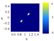
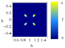
$\omega=6meV$

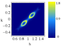
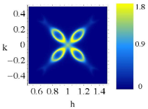
$\omega=36meV$

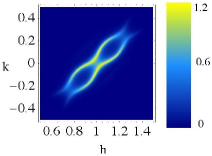
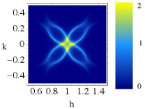
$\omega=55meV$

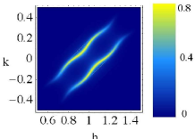
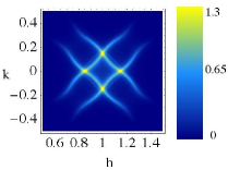
$\omega=80meV$

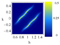
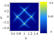
$\omega=120meV$

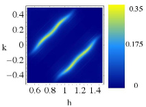
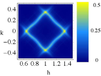
$\omega=160meV$

Figure 5: Plots of the scattering intensity in ordering Scenario I as a function of $h$ and $k$ (reduced lattice units) for a number of energies. At each energy the response is presented for both a single ladder array (left hand figure) and two ladders arrays orientated at $90^{o}$ relative to one another (right hand figure). The parameters employed here are discussed in Appendix A1.

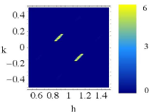
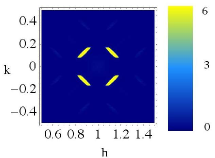
$\omega=6meV$

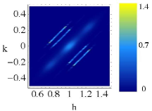
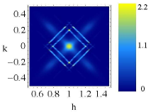
$\omega=36meV$

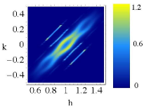
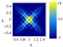
$\omega=55meV$

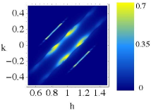
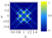
$\omega=80meV$

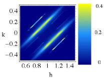
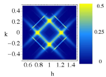
$\omega=120meV$

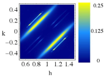
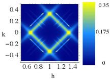
$\omega=160meV$

Figure 6: Plots of the scattering intensity in ordering Scenario II as a function of $h$ and $k$ (reduced lattice units) for a number of energies. The presentation scheme is the same as Fig. 5. The parameters for the ladders used here are discussed in Appendix A2.

V Magnetic Response of Coupled Ladders

In this section we elaborate upon the magnetic response of the coupled ladders in the first two scenarios presented in Section IV C. In particular we will show that either of these scenarios is compatible with the observed gross features of the magnetic response of $\rm La_{1.875}Ba_{0.125}CuO_{4}$ and $\rm La_{2-x}Sr_{x}CuO_{4}$.

We first consider constant energy slices of the spin response as a function of wavevector. Choosing the same energies reported in Ref. tran_nat , we plot the results in Figures 4 and 5, where the reduced lattice units $h$ and $k$ are defined via tran_nat

$$h=\frac{q_{x}+q_{y}}{2\pi};~{}~{}~{}k=\frac{q_{y}-q_{x}}{2\pi}.$$ (30)

In both figures we show the spin response resulting for a single plane of ladders (left figure of each pair) and for a pair of planes of ladders orientated at $90^{o}$ degrees to one another (right figure of each pair). The second arrangement (pictured in Fig. 3) corresponds to how stripes order in $\rm La_{1.875}Ba_{0.125}CuO_{4}$ and $\rm La_{1.82}Sr_{0.18}CuO_{4}$, and so is the one relevant for comparison with experiment. We, however, include the response of a single plane as it is here that the magnetic response of the two ordering scenarios most sharply distinguish themselves.

In Figure 5, Scenario I is presented, the case where the magnetic order develops perpendicular to the ladder, i.e. at wavevector $(\pi,\pi\pm\frac{\pi}{4})$. At the lowest of energies shown, $\omega=6meV$, we find for a single plane of ladders, a pair of incommensurate spin waves dispersing at the incommensurate wavevectors $(h,k)=(1\pm 1/8,\pm 1/8)$. In the response for two planes, we then observe a second pair of spin waves, rotated by $90^{o}$ relative to the first. The dispersions cones of the wavevectors are elongated along the diagonal, a consequence of the anisotropy between inter- and intra-ladder couplings ($J_{c}$ and $J$). As we increase in energy to $\omega=36meV$, the spin waves disperse outwards. We see that spectral weight of the cones in anisotropically distributed, with more weight being found on the side of the cone nearest to $(\pi,\pi)$. Thus we see that as we increase in energy, the spectral weight appears to move away from the incommensurate points towards $(\pi,\pi)$. By $\omega=55meV$, the energy corresponding to the gap in the undoped ladders, the cones have begun to overlap. This overlap is enhanced for the response of a pair of planes, leading to the most intense response coming from $(\pi,\pi)$. As energy is further increased, we observe a rotation in the intensity by $45^{o}$ in the pair plane response (compare energies $\omega=36meV$ and $\omega=80meV$). The rotation results from the dominance of the spin response of the half-filled ladders, which for a single plane form lines of intensity. With a pair of relatively orientated planes, the lines cross, leading to the four peaks. As we increase energy further, the peaks in the two-plane response disperse outwards while at the same time losing intensity. By $\omega=160meV$, the spin response has become both comparatively broad and weak.

In Figure 6, we plot the magnetic response of the second scenario where order appears parallel to the ladders. At the lowest energy shown, $\omega=6meV$, we again find incommensurate spin waves, which now appear, for a single plane, at $(h,k)=(1\mp 1/8,\pm 1/8)$. The spin waves, in this case, are much more strongly anisotropic. But we believe this is a feature of the details of the ladder susceptibilities, not a fundamental feature of the model. While the response at $\omega=6meV$ for this ordering pattern is rotated by $90^{0}$ relative to where the order develops perpendicular to the ladders, the response for a pair of planes is qualitatively no different in the two cases. As we increase in energy, the spin waves appearing at low energies evolve into the response of a set of nearly uncoupled doped ladders. Accompanying this evolution is a separate development of spectral weight at $(\pi,\pi)$. The presence of inelastic spectral weight of $(\pi,\pi)$ is a consequence of the competition in this scenario between order developing at $q_{x}=\pi$ (the location of coherent mode on the doped ladder) and order developing incommensurately at $q_{x}=3\pi/4$ and $5\pi/4$ (the location of the quasi-coherent mode on the undoped ladder). Though in this case order is favored at the incommensurate wavevector, the commensurate order remains pre-emergent and so appears at finite energy values. Taken together, these two effects again give the appearance of a movement of spectral weight towards $(\pi,\pi)$. As we continue further up in energy, the response of the half-filled ladders again begins to dominate, with a peak in the intensity near $(\pi,\pi)$ (see $\omega=55meV$ in Fig. 6). The dominance of the half-filled ladders then continues to higher energies ($\omega=80meV$ and above), and consequently, the response takes on the same form as that of Figure 5.

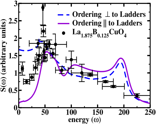
Figure 7: Integrated intensity, $S(\omega)$, of the coupled ladder system in the two ordering scenarios. For comparison, we plot these results against Ref. tran_nat . The parameters are the same as for Figs. 5 and 6.

While our model of coupled ladders finds reasonable approximates to the observations on LBCO of Ref. tran_nat, , it produces features at higher energies that are typically much sharper than those actually observed. This however is not surprising. The RPA approximation we employ will generically underdamp high energy stripe-like correlations.

As another measure of the response of the two scenarios, we compute at fixed energy the $q$-integrated intensity, $S(\omega)$, of the coupled ladders. This quantity is defined by

$$S(\omega)=\int d^{2}q{\rm Im}\chi(\omega,q_{x},q_{y}).$$ (31)

We plot the results in Figure 5 for the two scenarios. We see we obtain a rough agreement. At low energies there is an increase in intensity corresponding to the development of incommensurate long range order. We also see an enhancement in the intensity at $J=50meV$ which corresponds to the spin gap of the half-filled ladders. This is to be expected as the excitation spectrum of the half-filled ladder is a single coherent mode and should have a strong response. For energies in excess of the spin gap, we then see a gradual decline in intensity in both the measured and computed responses. The primary difference between the two scenarios lies in the total amount of spectral weight found at low energies. But this difference is not fundamental and rather is a product of particular choices made to describe the susceptibilities of the individual ladders in both cases.

VI Discussion

We approached this work with three primary motivations: i) to understand whether a model of coupled ladders with alternating levels of doping is compatible with the observed spin response in $\rm La_{1.875}Ba_{0.125}CuO_{4}$ and $\rm La_{2-x}Sr_{x}CuO_{4}$; ii) to suggest that distinct patterns of magnetic ordering can lead to the same set of experimental observations in these particular cuprates; and iii) to explore the specific role that the internal dynamics of the doped regions play in the development of stripe order. We deal with each in turn.

The observations of Ref. tran_nat of the inelastic spin response in $La_{1.875}Ba_{0.125}CuO_{4}$ has several basic features. At zero energy there appear inelastic incommensurate spin waves at the four wavevectors, $Q=(\pi,\pi(1\pm 1/4))$ and $Q=(\pi(1\pm 1/4),\pi)$. At small but finite energies (up to $50meV$), the intensity associated with these spin waves appears to propagate away from these incommensurate points and inwards towards $(\pi,\pi)$. At higher energies, the movement of the spectral weight reverses direction, propagating outward, but with peaks rotated by $45^{o}$ relative to the low energy spin waves.

In the previous sections we have show that there exist two coupled ladder scenarios that qualitatively reproduce these features. The two scenarios are distinguished by the direction in which the incommensurate order develops, either parallel or perpendicular to the direction of the ladder. Nonetheless in both scenarios we find magnetic order at the four incommensurate wavevectors (in bi-planar systems). In both, we have a movement of spectral weight towards $(\pi,\pi)$ as energy moves upwards to $50meV$. And for energies greater than $50meV$, the spin response of both scenarios, dominated by the coherent mode of the undoped ladder, yields the same outward (from $(\pi,\pi)$) propagation of spectral weight rotated by $45^{o}$ relative to the location of the low energy spin waves.

While the two scenarios are qualitatively similar, there are quantitative differences. The low energy spectral features present in Scenario II (ordering along the ladder) are far more anisotropic than those in Scenario I (ordering perpendicular to the ladder). This however is less a fundamental feature of Scenario II and more a consequence of the use of the field theoretic treatment of the doped ladders at medium energies. At such energies, the neglected non-relativistic band curvature will moderate anisotropic features. A more fundamental difference is the manner in which spectral weight moves inwards towards $(\pi,\pi)$ as energies are increased to $50meV$. In Scenario I, this movement is a consequence of expanding spin wave cones possessing an unequal distribution of spectral weight. In Scenario II, the weight moves towards $(\pi,\pi)$ due to the spectral features present on the uncoupled doped ladder together with nascent ordering at $(\pi,\pi)$. This ordering, discussed briefly in Section IV C, while not elastic, cannot be entirely suppressed at higher energies.

While the primary focus of this work has been on static stripe order of the kind observed in $\rm La_{1.875}Ba_{0.125}CuO_{4}$, one may ask whether our model of coupled ladders might be applicable more generally to incommensurate magnetic excitations in the cuprates. At least to some degree it does. In slightly overdoped LSCO ($\rm La_{1.84}Sr_{0.16}CuO_{4}$), nascent incommensurate long range order has been reported lake1 ; christensen ; vignolle . Specifically, neutron scattering experiments observe a broad peak centered about $11meV$ in the scattering intensity at the incommensurate wavevector $(h,k)=(1\pm 1/8,\pm 1/8)$ (see Figure 8). (A similar phenomena is seen in $\rm La_{1.82}Sr_{0.18}CuO_{4}$ tran_lsco .) This magnetic response can be understood through our model of ladders with an interladder coupling, $J_{c}$, less than its critical ordering value, $J_{crit}$. The responses for $J_{c}<J_{crit}$ for both scenarios ($||$ and $\perp$) are pictured in Figure 8. For comparison we have plotted the corresponding responses for $J_{c}=J_{crit}$ where long range order is fully developed. There, as $\omega$ is decreased, the response diverges at the incommensurate wavevector.

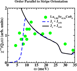
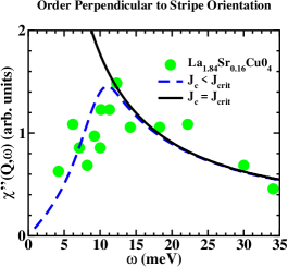
The intensity of the spin response at the incommensurate ordering wavevector, $Q$, for the two ordering scenarios. We show the response for both sub-critical and critical values of the interladder coupling, $J_{c}$. We compare this with the maximal intensity in $\rm La_{1.84}Sr_{0.16}CuO_{4}$ for $T>T_{c}$ measured in Ref. christensen . For ordering perpendicular to the ladders the parameters are the same as those found in Figs. 5 and 7. For the second scenario, as explained in Appendix A2, the parameters used differed from those employed in Figs. 6 and 7.

The compatibility of both stripe ordering scenarios we discuss with the observed spin response in both $\rm La_{1.875}Ba_{0.125}CuO_{4}$ and $\rm La_{1.84}Sr_{0.16}CuO_{4}$ trades on the bilayer ordering structure of stripes in these two materials where the stripes in adjacent copper-oxide planes are orientated perpendicular to one another. While the spin responses of stripes in a single plane is much different in the two scenarios, once rotated and superimposed, the responses become qualitatively the same.

Experimental evidence beyond the spin response in these compounds provides only limited evidence allowing one to distinguish between these two scenarios. In Scenario I extended to general levels of doping ZEK , incommensurate wave vectors of charge and spin density waves are arranged perpendicular to the direction of stripes and are related to each other via

$${\bf Q^{I}}_{ch}=(0,\pm 4\pi x),~{}~{}{\bf Q^{I}}_{s}=(\pi,\pi\pm 2\pi x),$$ (32)

where $x$ denotes the doping. In contrast, in Scenario II stripes are found in the form of coupled two leg ladders, independent of doping, gaining in this fashion, magnetic energy. Here the pattern of incommensuration appears as

$${\bf Q^{II}}_{ch}=(0,\pm\frac{\pi}{2}),~{}~{}~{}{\bf Q^{II}}_{s}=(\pi\pm 2\pi x,\pi).$$ (33)

The behavior of incommensurate spin order at $Q_{sx}=\pi\pm 2\pi x$ as a function of doping directly tracks the wavevector where low energy quasi-coherent modes exist in the doped ladder.

To distinguish between these two scenarios we must then focus upon the charge incommensuration. However only the doping dependence of the magnetic incommensuration has been carefully studied (see tran_rev and references therein). The experiments show that the spin incommensuration is proportional to the doping $x$ for $x<1/8$ and then saturates. On the other hand charge peaks have been observed only for a narrow range of dopings and only in stripe stabilized cuprates (in La_1.5Nd_0.4Sr_0.1CuO₄ Nd , La_1.475Nd_0.4Sr_0.125CuO₄ john , La_1.45Nd_0.4Sr_0.15CuO₄ nie , and La_1.875Ba_0.125CuO₄ abba ). While the observed charge incommensuration, $Q_{ch}$, changes as a function of $x$ (and so is supportive of Scenario I), it does so weakly, i.e. the change in $Q_{ch}$ is governed by $\delta Q_{ch}=c\delta x$ with $c\sim 0.5$. One might then want to conclude that Scenario II remains a possibility, at least for dopings in a narrow window about $x\sim 0.125$. The situation is similarly ambiguous for $\rm YBa_{2}Cu_{3}O_{6+x}$. Here distinct measurements of the phonon anomaly support alternatively Scenario I mook ; keimer1 and Scenario II pint .

Scenario II is viable away from 1/8 doping in another fashion. In Ref. john1, , the behaviour of the incommensuration as a function of $x$ is explained by invoking stripe spacing disorder. Modifying this approach, we can imagine stripe spacing disorder producing changes in the charge incommensuration while the magnetic incommensuration arises from the doped ladder quasi-coherent mode (and so again is parallel to the stripe). This then yields a incommensuration pattern

$${\bf Q^{II^{\prime}}}_{ch}=(0,\pm 4\pi x),~{}~{}~{}{\bf Q^{II^{\prime}}}_{s}=(\pi\pm 2\pi x,\pi),$$ (34)

which gives Scenario I’s charge incommensuration but Scenario II’s magnetic incommensuration.

Independent of either scenario, our modeling efforts show the value of taking into account the doped region of the copper-oxide planes. In coupling together the ladders, we employed antiferromagnetic couplings but were nonetheless able to explain the appearance of incommensurate order and the corresponding $\pi$-phase shift in magnetic order. If the doped regions were instead considered inert, a ferromagnetic coupling would have to be assumed between adjacent doped ladders kruger ; vojta ; uhrig ; carlson .

While we have focused on magnetism here, models of coupled ladders have promising superconducting properties. It has already been established that a model of a uniform array of coupled half-filled ladders possesses narrow arcs of quasi-particles which have an instability towards d-wave superconductivity konricetsv . Ultimately this is a consequence of the presence of nascent d-wave superconducting order on the component ladders Fisher ; Fabrizio . However these arcs are highly anisotropic with an alignment parallel to the ladders. A question that then should be asked is whether a model of an array of ladders with alternating doping can do better. Can such a model produce arcs aligned at $45^{o}$? If it could, it would fill in an important piece of the puzzle of how 1/8-doped LBCO can exhibit both stripe order together with nodal quasi-particles ARPES .

Appendix A Susceptibilities of the Doped Ladders

We extract the susceptibilities of doped ladder from a field theoretic reduction of the ladders (Ref. FabRob ). The corresponding field theory takes the form of the SO(6) Gross Neveu model supplemented by a U(1) Luttinger liquid describing the charge sector. Though such a description captures low energy features of the system, it leaves us with ambiguities concerning the amplitudes of the correlation functions. It is these ambiguities which give rise to the possibility of different ordering scenarios described in the text.

The field theory predicts the following general form for the susceptibilities:

$$\chi^{\rm d}_{0}(\omega,q) = \frac{3}{8}A_{11}J_{1}(\omega,q);$$ (35)

$$\chi^{\rm d}_{2k_{F+}}(\omega,q) = \frac{3}{8}A_{12}\bigg{(}J_{2}(\omega,q+2K_{F+})+J_{2}(\omega,q-2K_{F+})\bigg{)};$$ (37)

$$\chi^{\rm d}_{2k_{F-}}(\omega,q) = \frac{3}{8}A_{12}\bigg{(}J_{2}(\omega,q+2K_{F-})+J_{2}(\omega,q-2K_{F-})\bigg{)};$$ (39)

$$\chi^{\rm d}_{k_{F+}-k_{F-}}(\omega,q) = \frac{3}{8}A_{31}\bigg{(}J_{1}(\omega,q+K_{F-}-K_{F+})+J_{1}(\omega,q-K_{F-}+K_{F+})\bigg{)};$$ (41)

$$\chi^{\rm d}_{k_{F+}+k_{F-}}(\omega,q) = \frac{3}{8}A_{32}\bigg{(}J_{3}(\omega,q+K_{F-}+K_{F+})+J_{3}(\omega,q-K_{F-}-K_{F+})\bigg{)}.$$ (43)

In these expressions $A_{ij}$ are amplitudes with dimensionality of momentum that are determined by short-distance physics. On the other hand $J_{i}$’s are functions dependent on long-distance physics that arise from the form of the matrix elements of the spin operators in the $SO(6)$ Gross-Neveu model. Different choice of the amplitudes, $A_{ij}$, determine what ordering scenario is realized.

The imaginary part of $J_{1}$ takes the form

$${\rm Im}J_{1}(\omega,q)=\frac{8v_{F}\tilde{q}^{2}}{(\omega^{2}-\tilde{q}^{2})^{3/2}}\frac{\theta(\omega-\sqrt{\tilde{q}^{2}+4m^{2}})}{(\omega^{2}-\tilde{q}^{2}-4m^{2})^{1/2}}$$ (44)

(45)

$$\ \times\ \exp\bigg{[}\int^{\infty}_{0}\frac{dx}{x}\frac{G_{c}(x)}{s(x)}\big{(}1-c(x)\cos(\frac{\theta_{12}x}{\pi})\big{)}\bigg{]},$$ (46)

where $\theta_{12}$ is given by

$$\theta_{12}=\cosh^{-1}(\frac{\omega^{2}-\tilde{q}^{2}-2m^{2}}{2m^{2}}),$$ (47)

and $\tilde{q}=v_{F}q$ where $v_{F}$ is the Fermi velocity of electrons in either the bonding or antibonding bands. Here $s(x)/c(x)\equiv\sinh(x)/\cosh(x)$ and

$$G_{c}(x)=\frac{e^{x/2}-1}{s(x)}.$$

The imaginary parts of $J_{2}$ and $J_{3}$ can be expressed more compactly as integrals over hypergeometric functions:

$$J_{2}(\omega,q) = \frac{v_{F}}{m^{2}}\int_{-\infty}^{\infty}d\theta\frac{s^{2}(\theta)}{\left[c(\theta)\right]^{\frac{4-K}{2}}}F\big{(}1-\frac{K}{4},1-\frac{K}{4},1,\frac{(\omega+\mbox{i}0)^{2}-\tilde{q}^{2}}{4m^{2}c^{2}(\theta)}\big{)}$$ (49)

$$\hskip 72.26999pt\exp\Big{\{}\int^{\infty}_{0}\frac{dx}{x}\frac{G_{s}(x)}{s(x)}[1-c(x)\cos(\frac{2\theta x}{\pi})]\Big{\}};$$

$$J_{3}(\omega,q) = \frac{v_{F}}{2g^{2}m^{2}}\exp\Big{(}-2\int^{\infty}_{0}\frac{dx}{x}\frac{G_{v}(x)}{s(x)}s^{2}(\frac{x}{4})\Big{)}F\bigg{(}1-\frac{K}{4},1-\frac{K}{4},1,\frac{(\omega+\mbox{i}0)^{2}-\tilde{q}^{2}}{2m^{2}}\biggr{)}$$ (55)

$$\hskip-36.135pt+\frac{2^{K/4}v_{F}}{\pi m^{2}}\int_{-\infty}^{\infty}d\theta\frac{1}{\left[c(\theta)\right]^{\frac{4-K}{2}}}\Big{[}\frac{s(2\theta)^{2}}{2c(2\theta)^{2}}+\frac{s(\theta)^{2}}{c(2\theta)^{2}}\Big{]}F\biggl{(}1-\frac{K}{4},1-\frac{K}{4},1,\frac{(\omega+\mbox{i}0)^{2}-\tilde{q}^{2}}{4m^{2}c^{2}(\theta)}\biggr{)}$$

$$\hskip 36.135pt\times\exp\Big{\{}\int^{\infty}_{0}\frac{dx}{x}\frac{G_{v}(x)}{s(x)}[1-c(x)\cos(\frac{2\theta x}{\pi})]\Big{\}},$$

where

$$G_{v}(x)=\frac{2}{1-e^{-2x}}\bigg{(}e^{-2x}(1-e^{x/2})-e^{-5x/2}(1-e^{2x})\bigg{)}.$$

Here $K$ is the Luttinger parameter governing the gapless total charge mode of the doped ladder and $g$ is a constant given by

$$g^{2}=\frac{2\sqrt{\pi}\Gamma(7/4)}{3\Gamma(5/4)}.$$

To evaluate the real parts of $J_{a}$ ($a=1,2,3$) we Kramers-Kronig transform the above expressions for ${\rm Im}J$:

$${\rm Re}J(\omega,q)=\frac{1}{\pi}\int^{D}_{-D}d\omega^{\prime}\frac{{\rm Im}J(\omega^{\prime},q)}{\omega-\omega^{\prime}}.$$ (56)

We equip the transformation with a cutoff, $D\sim v_{F}/a$, to reflect the fact the imaginary parts of $J_{2}$ and $J_{3}$ are only accurate representations of the low energy sector of the ladders. To determine the real parts of $J_{2/3}$ we perform the transformation over a frequency interval roughly corresponding to this sector. Our results, however, are insensitive to the exact value of $D$.

A.1 Scenario I: Ordering Perpendicular to the Ladders

To be able to produce the analysis of ordering perpendicular to the ladders (Scenario I – Figs. 5, 7, and 8) we had to fix the parameters $v_{F}A_{ij}/m^{2}$ and determine the value of spin gap $m$. In Ref. FabRob , we did this through a comparison with an RPA analysis of a Hubbard ladder with an onsite U repulsion. The value of the spin gap $m$ is related to the bandwidth, $t$, the Hubbard interaction, $U$, and the Fermi velocity $v_{F}$. For $t\approx U$ we chose $t=4ev$ and for $v_{F}=350meVa$ (where a is the lattice spacing). $v_{F}$ is not readily available as its (strong) renormalization due to interactions is a two-loop effect. But the value we employed is commensurate with what is measured in the cuprates radu . As discussed in Ref. FabRob , knowledge of $t$ alone is enough to fix the value of the gap, $m=26{\rm meV}$, using a field theory analysis for doped ladders klls together with the values of the gap on the ladder as determined from DMRG at half-filling eric ; weihong . From this same field theory analysis, the Luttinger parameter can be determined as $K=0.945$. In Figs. 5 and 7 we couple the ladders together with a strength just below that of the critical interladder coupling as determined from our RPA analysis – here $J_{crit}=16.05$meV. We choose the value of $J$ on the undoped ladders to be $100meV$ so as to match experimental observations of the location of the neck of the hourglass describing the evolution of excitations in $La_{1.875}Ba_{0.125}CuO_{4}$ tran_nat . Furthermore to partially mimic the broadening seen in experiment, we broadened the spectral function of the undoped ladders by assuming a lifetime of $0.1J$.

The constants, $A_{ij}$, that appear in Eqn. (35) are not determined by the field theory treatment itself but must be accessed through separate considerations. In Ref. FabRob we, through a comparison with a RPA analysis of a Hubbard ladder with an onsite U repulsion, were able to provide tentative values for the $A_{ij}$’s.

A.2 Scenario II: Ordering Parallel to the Ladders

Since the amplitudes $A_{ij}$ are determined by processes with energies of the order of the bandwidth, we have a liberty of choice. For Scenario I we have chosen the high energy physics as in a simple doped Hubbard ladder with a point-like interaction and $U\sim t$. One can imagine that some other lattice realization generates a set of amplitudes such that the spectral weight associated with the quasi-coherent spin excitation dominates. To develop this scenario, we thus focus on this excitation to the exclusion of contributions coming from two excitation scattering continua. Specifically we set $A_{11}=A_{12}=A_{31}=0$, leaving only $A_{32}$ finite, and take $J_{3}$ to equal

$$J_{3}(\omega,k)=\frac{v_{F}}{2g^{2}m^{2}}\exp\bigg{(}-2\int^{\infty}_{0}\frac{dx}{x}\frac{G_{v}(x)}{\sinh(x)}\sinh^{2}(\frac{x}{4})\bigg{)}F\bigg{(}1-\frac{K}{4},1-\frac{K}{4},1,\frac{\omega^{2}-\tilde{k}^{2}}{2m^{2}}\biggr{)}.$$ (57)

As such, $J_{3}$ now represents a coherent mode broadened by the presence of gapless charge excitations.

For this scenario, in order to produce the spin response at constant energy in Fig. 6 and the integrated intensity in Fig. 7, we must choose the ratio of $v_{f}/m$ to be sufficiently large in order to guarantee Scenario II prevails over Scenario III. To ensure this we chose $v_{f}=250{\rm meV}a$, and the lattice bandwidth to be $t=1000meV$ (and thus via Refs. klls ; eric ; weihong , $m=0.0065t=6.5meV$). Both the parameters used for the undoped ladder and the Luttinger parameter describing charge excitations on the doped ladders where the same as in Scenario I (appendix A1).

In order to produce the results displayed in the left hand side of Fig. 8 (discussing the strength of the inelastic signal in $\rm La_{1.86}Sr_{0.14}CuO_{4}$ at the incommensurate wave vector), we took instead $v_{f}=360{\rm meV}a$ and $t=3000meV$. This in turn moved the gap scale on the doped ladders to $m=21{\rm meV}$, high enough so that it did not interference with the low energy signal marking nascent incommensurate order.

References

- (1) J. G. Bednorz and K. A. Müller, Z. Phys. B: Condens. Matter 64, 189 (1986).
- (2) A. R. Moodenbaugh, Y. Xu, M. Suenaga, T. J. Folkerts, and R. N. Shelton, Phys. Rev. B 38 (1988) 4596.
- (3) M. Fujita, H. Goka, and K. Yamada, J. M. Tranquada, and L. P. Regnault, Phys. Rev. B 70 (2004) 104517.
- (4) J. M. Tranquada, H. Woo, T. G. Perring, H. Goka, G. D. Gu, G. Xu, M. Fujita, and K. Yamada, Nature 429, 534 (2004).
- (5) P. Abbamonte, A. Rusydi, S. Smadici, G. D. Gu, G. A. Sawatzky, and D. L. Feng, Nature Phys. 1, 155 (2005).
- (6) J. M. Tranquada, Neutron Scattering Studies of Antiferromagnetic Correlations in Cuprates appearing in Handbook of High-Temperature Superconductivity, ed. J. R. Schrieffer and J. S. Brooks, Springer New York (2005).
- (7) Stripe phases are also found in allied compounds to the cuprates, for example the nickelates, . See for example J. M. Tranquada, D. J. Buttrey, V. Sachan, and J. E. Lorenzo, Phys. Rev. Lett. 73, 1003 (1994).
- (8) P. Dai, H. A. Mook, R. D. Hunt, and F. Doǧan, Phys. Rev. B 63, 054525 (2001).
- (9) H. A. Mook, P. Dai, F. Doǧan, and R. D. Hunt, Nature 404, 729 (2000).
- (10) V. Hinkov, S. Pailhès, P. Bourges, Y. Sidis, A. Ivanov, A. Kulakov, C. T. Lin, D. P. Chen, C. Bernhard, and B. Keimer Nature 430, 650 (2004).
- (11) V. Hinkov, P. Bourges, S. Pailhès, Y. Sidis, A. Ivanov, C. D. Frost, T. G. Perring, C. T. Lin, D. P. Chen, and B. Keimer, Nature Physics 3, 780 (2007).
- (12) See Ref.(mook, ) above for evidence to this effect. We do note however that Ref. pint has reported observations of this same phonon anomaly indicating that the incommensurate spin modulation is found along the stripes.
- (13) L. Pintschovius, W. Reichardt, M. Kläser, T. Wolf, and H. v. Löhneysen, Phys. Rev. Lett. 89, 037001 (2002).
- (14) K. Yamada, C. H. Lee, K. Kurahashi, J. Wada, S. Wakimoto, S. Ueki, H. Kimura, Y. Endoh, S. Hosoya, G. Shirane, R. J. Birgeneau, M. Greven, M. A. Kastner, and Y. J. Kim, Phys. Rev. B 57, 6165 (1998).
- (15) M. Fujita, K. Yamada, H. Hiraka, P. M. Gehring, S. H. Lee, S. Wakimoto, and G. Shirane, Phys. Rev. B 65, 064505 (2002).
- (16) F. Krüger and S. Scheidl, Phys. Rev. B 67, 134512 (2003).
- (17) M. Vojta and T. Ulbricht, Phys. Rev. Lett. 93, 127002 (2004).
- (18) G.S. Uhrig, K.P. Schmidt and M. Grüninger, Phys. Rev. Lett. 93, 267003 (2004).
- (19) D. X. Yao, E. W. Carlson, D. K. Campbell, Phys. Rev. B 73, 224525 (2006); D. X. Yao, E. W. Carlson, Phys. Rev. B 77, 024503 (2008).
- (20) In particular, the low energy field theoretic treatment that we employ to characterize the spin response of the doped ladder does not uniquely fix the real part of the susceptibility, a quantity dependent upon high energy non-universal physics.
- (21) Guangyong Xu, J. M. Tranquada, T. G. Perring, G. D. Gu, M. Fujita, and K. Yamada, Phys. Rev. B 76, 014508 (2007).
- (22) M. Granath, V. Oganesyan, S.A. Kivelson, E. Fradkin and V. Emery, Phys. Rev. Lett. 87, 167011 (2001); M. Granath, V. Oganesyan, D. Orgad and S.A. Kivelson, Phys. Rev. B65, 184501 (2002).
- (23) T. Valla, A.V. Fedorov, J. Lee, J.C. Davis and G.D. Gu, Science 314, 1914 (2006); M.R. Norman, A. Kanigiel, M. Randeria, U. Chatterjee and J.C. Campuzano, Phys. Rev. B 76, 174501 (2007).
- (24) M. Fabrizio, Phys. Rev. B 48, 15838 (1993).
- (25) H. L. Lin, L. Balents and M. P. A. Fisher, Phys. Rev. B 58, 1794 (1998).
- (26) E. Arrigoni, E. Fradkin and S. Kivelson, Phys. Rev. B69, 214519 (2004).
- (27) R. M. Konik, T. M. Rice, and A. M. Tsvelik, Phys. Rev. Lett. 96, 086407 (2006).
- (28) S. Notbohm, P. Ribeiro, B. Lake, D. A. Tennant, K. P. Schmidt, G. S. Uhrig, C. Hess, R. Klingeler, G. Behr, B. B chner, M. Reehuis, R. I. Bewley, C. D. Frost, P. Manuel, and R. S. Eccleston, Phys. Rev. Lett. 98, 027403 (2007).
- (29) B. Lake, G. Aeppli, T. E. Mason, A. Schr der, D. F. McMorrow, K. Lefmann, M. Isshiki, M. Nohara, H. Takagi, and S. M. Hayden, Nature 400 43 (1999).
- (30) N. B. Christensen, D. F. McMorrow, H. M Rønnow, B. Lake, S. M. Hayden, G. Aeppli, and T. G. Perring, Phys. Rev. Lett. 93, 147002 (2004).
- (31) B. Vignolle, S. M. Hayden, D. F. McMorrow, H. M. Rønnow, B. Lake, C. D. Frost, and T. G. Perring, Nature Physics 3, 163 (2007).
- (32) J. M. Tranquada, C. H. Lee, K. Yamada, Y. S. Lee, L. P. Regnault, and H. M. Rønnow, Phys. Rev. B 69, 174507 (2004).
- (33) T. Barnes and J. Riera, Phys. Rev. B 50, 6817 (1994).
- (34) K.P. Schmidt and G.S. Uhrig, Mod. Phys. Lett. B19, 1179 (2005).
- (35) O. Zachar, S. A. Kivelson and V. J. Emery, Phys. Rev. B57, 1422 (1998).
- (36) T. Niemöller, N. Ichikawa, T. Frello, H. Hn̈nerfeld, N. H. Andersen, S. Uchida, J. R. Schneider, J. M. Tranquada, Euro. Phys. J B 12, 509 (1999).
- (37) J. M. Tranquada, B. J. Sternlieb, J. D. Axe, Y. Nakamura, and S. Uchida, Nature 375, 561 (1995). Phys. Rev. Lett. 85, 1738 (2000).
- (38) N. Ichikawa, S. Uchida, J. M. Tranquada, T. Niemöller, P. M. Gehring, S.-H. Lee, and J. R. Schneider, Phys. Rev. Lett. 85, 1738 (2000).
- (39) J. M. Tranquada, N. Ichikawa, and S. Uchida, Phys. Rev. B 59, 14712 (1999).
- (40) F. H. L. Essler and R. M. Konik, Phys. Rev. B 75, 144403 (2007).
- (41) R. M. Konik, F. Lesage, A. Ludwig, and H. Saleur, Phys. Rev. B 61, 4983 (2000).
- (42) R. Coldea, S. M. Hayden, G. Aeppli, T. G. Perring, C. D. Frost, T. E. Mason, S.-W. Cheong, and Z. Fisk, Phys. Rev. Lett. 86, 5377 (2001).
- (43) E. Jeckelmann, D.J. Scalapino and S.R. White, Phys. Rev. B58, 9492 (1998).
- (44) Z. Weihong, J. Oitmaa, C.J. Hamer and R.J. Bursill, J. Phys. Cond. Matt. 13, 433 (2001).