Abruption of entanglement and quantum communication through noise channels

Abstract

We investigate the dynamics of two qubits state through the Bloch channel. Starting from partially entangled states as input state, the output states are more robust compared with those obtained from initial maximally entangled states. Also the survivability of entanglement increased as the absolute equilibrium values of the channel increased or the ratio between the longitudinal and transverse relaxation times gets smaller. The ability of using the output states as quantum channels to perform quantum teleportation is investigated. The useful output states are used to send information between two users by using the original quantum teleportation protocol.

Keywords: Qubit, Entanglement, Channels, Communication.

1 Introduction

Nowadays information can be stored, transmitted and manipulated by qubits. The most important kinds of qubits are the entangled ones. Although it is possible to generate useful entangled states for quantum information purposes, decoherence processes result in shortening their survival. This, in turn affects efficiency of performing such tasks as in quantum teleportation [1, 2]. So, finding a robust scheme for quantum information tasks is very important [3].

Decoherence represents an inevitable process which causes entanglement to be fragile. There is a new kind of decay called the death of entanglement resulting from classical noise has been discussed recently [4, 5, 6]. In reality there are several ways causing the indescribable decoherence. For example, the interaction of qubits with its surroundings [7], device imperfections [8, 9], the decay due to spontaneous, emission and the noisy channel [10].

So, investigating the dynamics of entanglement in the presence of decoherence is one of the most important tasks in quantum computation and information. In the present work, we examine some intrinsic properties of the dynamics of a two qubit state passing through Bloch channels. The decoherence of entanglement and information in these types of channel has been investigated [11, 12], where, the case of only one qubit passing through the Bloch channel is studied. In our contribution, we assume that there is a source that supplies us with a two qubit state. One qubit is sent to the user, Alice and the second qubit is sent to Bob. Then the two qubits are forced to be sent through the Bloch channel. Our study focus on the properties of the output state from different directions as we shall see later.

The paper is organized as follows: In Sec.$2$, the evolution of a general two-qubit state passes through Bloch channel is examined analytically. Sec.$3$ is devoted for numerical calculations, where the survival degree of entanglement is quantified and the phenomena of the decay and sudden death of entanglement are examined. Use the output state for quantum teleportation is studied in Sec.$4$. Finally, a conclusion is given in Sec$.5$.

2 The Model

The characterization of the 2-qubit states produced by some source requires experimental determination of 15 real parameters. Each qubit is determined by $3$ parameters, representing the Bloch vectors, and the other $9$ parameters represent the correlation tensor. Analogs of Pauli’s spin operators are used for the description of the individual qubits; the set $\sigma_{1},\sigma_{2},\sigma_{3}$ for Alice’s qubit and $\tau_{1},\tau_{2},\tau_{3}$ for Bob’s qubit. Any two qubit state is described by [13, 14, 15],

$$\rho_{ab}=\frac{1}{4}(1+\mathord{\buildrel\lower 3.0pt\hbox{$\scriptscriptstyle\rightarrow$}\over{A}}\cdot{\sigma^{\raisebox{2.0pt}[0.0pt]{$\scriptstyle\downarrow$}}}+\mathord{\buildrel\lower 3.0pt\hbox{$\scriptscriptstyle\rightarrow$}\over{B}}\cdot{\tau^{\raisebox{2.0pt}[0.0pt]{$\scriptstyle\downarrow$}}}+\mathord{\buildrel\lower 3.0pt\hbox{$\scriptscriptstyle\rightarrow$}\over{\sigma}}\cdot\mathord{\begin{picture}(12.0,12.0)(-1.0,0.0)\put(-2.0,10.0){\makebox(0.0,0.0)[t]{$\scriptscriptstyle\downarrow$}} \put(-2.0,11.0){\makebox(0.0,0.0)[l]{$\scriptscriptstyle\longrightarrow$}} \put(5.0,0.0){\makebox(0.0,0.0)[b]{$C$}} \end{picture}}\cdot{\tau^{\raisebox{2.0pt}[0.0pt]{$\scriptstyle\downarrow$}}}),$$ (1)

where $\mathord{\buildrel\lower 3.0pt\hbox{$\scriptscriptstyle\rightarrow$}\over{\sigma}}$ and $\mathord{\buildrel\lower 3.0pt\hbox{$\scriptscriptstyle\rightarrow$}\over{\tau}}$ are the Pauli’s spin vector of the first and the second qubits respectively. The statistical operator for the individual qubit are specified by their Bloch vectors, $\mathord{\buildrel\lower 3.0pt\hbox{$\scriptscriptstyle\rightarrow$}\over{A}}=\left\langle\mathord{\buildrel\lower 3.0pt\hbox{$\scriptscriptstyle\rightarrow$}\over{\sigma}}\right\rangle$ and $\mathord{\buildrel\lower 3.0pt\hbox{$\scriptscriptstyle\rightarrow$}\over{B}}=\left\langle\mathord{\buildrel\lower 3.0pt\hbox{$\scriptscriptstyle\rightarrow$}\over{\tau}}\right\rangle$. The cross dyadic $\mathord{\begin{picture}(12.0,12.0)(-1.0,0.0)\put(-2.0,10.0){\makebox(0.0,0.0)[t]{$\scriptscriptstyle\downarrow$}} \put(-2.0,11.0){\makebox(0.0,0.0)[l]{$\scriptscriptstyle\longrightarrow$}} \put(5.0,0.0){\makebox(0.0,0.0)[b]{$C$}} \end{picture}}$ is represented by a $3\times 3$ matrix. it describes the correlation between the first qubit, $\rho_{a}=tr_{b}\{\rho_{ab}\}=\frac{1}{2}(1+\mathord{\buildrel\lower 3.0pt\hbox{$\scriptscriptstyle\rightarrow$}\over{A}}\cdot{\sigma^{\raisebox{2.0pt}[0.0pt]{$\scriptstyle\downarrow$}}})$ and the second qubit $\rho_{b}=tr_{a}\{\rho_{ab}\}=\frac{1}{2}(1+\mathord{\buildrel\lower 3.0pt\hbox{$\scriptscriptstyle\rightarrow$}\over{B}}\cdot{\tau^{\raisebox{2.0pt}[0.0pt]{$\scriptstyle\downarrow$}}})$. The Bloch vectors and the cross dyadic are given by

$$\mathord{\buildrel\lower 3.0pt\hbox{$\scriptscriptstyle\rightarrow$}\over{A}} = (A_{1},A_{2},A_{3}),\quad\mathord{\buildrel\lower 3.0pt\hbox{$\scriptscriptstyle\rightarrow$}\over{B}}=(B_{1},B_{2},B_{3}),\quad\mbox{and}~{}\mathord{\begin{picture}(12.0,12.0)(-1.0,0.0)\put(-2.0,10.0){\makebox(0.0,0.0)[t]{$\scriptscriptstyle\downarrow$}} \put(-2.0,11.0){\makebox(0.0,0.0)[l]{$\scriptscriptstyle\longrightarrow$}} \put(5.0,0.0){\makebox(0.0,0.0)[b]{$C$}} \end{picture}}=\left(\begin{array}[]{ccc}c_{11}&c_{12}&c_{13}\\ c_{21}&c_{22}&c_{23}\\ c_{31}&c_{32}&c_{33}\end{array}\right)$$ (5)

Let us consider that each qubit is forced to pass in a Bloch channel. These channels are defined by the Bloch equations [11], for the first qubit,

$$\frac{d}{dt}\left\langle\sigma_{1}\right\rangle_{t} = -\frac{1}{T_{2a}}\left\langle\sigma_{1}\right\rangle_{t},~{}\frac{d}{dt}\left\langle\sigma_{2}\right\rangle_{t}=-\frac{1}{T_{2a}}\left\langle\sigma_{2}\right\rangle_{t},$$

$$\frac{d}{dt}\left\langle\sigma_{3}\right\rangle_{t} = -\frac{1}{T_{1a}}(\left\langle\sigma_{3}\right\rangle_{t}-\left\langle\sigma_{3}\right\rangle_{eq}),$$ (6)

while for the second qubit, they are given by

$$\frac{d}{dt}\left\langle\tau_{1}\right\rangle_{t} = -\frac{1}{T_{2b}}\left\langle\tau_{1}\right\rangle_{t},~{}\frac{d}{dt}\left\langle\tau_{2}\right\rangle_{t}=-\frac{1}{T_{2b}}\left\langle\tau_{2}\right\rangle_{t},$$

$$\frac{d}{dt}\left\langle\tau_{3}\right\rangle_{t} = -\frac{1}{T_{1b}}(\left\langle\tau_{3}\right\rangle_{t}-\left\langle\tau_{3}\right\rangle_{eq}),$$ (7)

where $T_{1i}$ and $T_{2i}$,  $i=a,b$ are the longitudinal and transverse relaxation times for Alice and Bob’s qubit, and $\left\langle\sigma_{3}\right\rangle_{eq}$,  $\left\langle\tau_{3}\right\rangle_{eq}$ are the equilibrium values of $\left\langle\sigma_{3}\right\rangle_{t}$ and $\left\langle\tau_{3}\right\rangle_{t}$ respectively. Now, we assume that Alice’s qubit $\rho_{a}$ and Bob’s qubit $\rho_{b}$ pass in the channels (2), and (2) respectively. Then the output state of the two qubit is defined by their new Bloch vectors

$$\tilde{\mathord{\buildrel\lower 3.0pt\hbox{$\scriptscriptstyle\rightarrow$}\over{A}}}(t) = (A_{1}\beta_{1},~{}-\beta_{1}A_{2},~{}\gamma_{1}A_{3}+(1-\gamma_{1})\left\langle\sigma_{3}\right\rangle_{eq}),$$

$$\tilde{\mathord{\buildrel\lower 3.0pt\hbox{$\scriptscriptstyle\rightarrow$}\over{B}}}(t) = (\beta_{2}B_{1},~{}-\beta_{2}B_{2},~{}\gamma_{2}B_{3}+(1-\gamma_{2})\left\langle\tau_{3}\right\rangle_{eq}).$$ (8)

In addition we present new correlation tensor

$$\tilde{C}_{11}(t) = \beta_{1}\beta_{2}C_{11},\quad\tilde{C}_{12}(t)=-C_{12}\beta_{1}\beta_{2},$$

$$\tilde{C}_{13}(t) = \beta_{1}\gamma_{2}C_{13}+\beta_{1}(1-\gamma_{2})\left\langle\sigma_{3}\right\rangle_{eq}A_{1},$$

$$\tilde{C}_{21}(t) = -C_{12}\beta_{1}\beta_{2},~{}\tilde{C}_{22}(t)=C_{22}\beta_{1}\beta_{2},$$

$$\tilde{C}_{23}(t) = -\beta_{1}\gamma_{2}C_{23}-\beta_{1}(1-\gamma_{2})\left\langle\tau_{3}\right\rangle_{eq}A_{2},$$

$$\tilde{C}_{31}(t) = \beta_{2}\gamma_{1}C_{31}+\beta_{2}(1-\gamma_{1})\left\langle\sigma_{3}\right\rangle_{eq}B_{1},$$

$$\tilde{C}_{32}(t) = -\beta_{2}\gamma_{1}C_{32}-\beta_{2}(1-\gamma_{1})\left\langle\sigma_{3}\right\rangle_{eq}B_{2},$$

$$\tilde{C}_{33}(t) = \gamma_{1}\gamma_{2}C_{33}+(1-\gamma_{1})(1-\gamma_{2})\left\langle\sigma_{3}\right\rangle_{eq}\left\langle\tau_{3}\right\rangle_{eq}$$ (9)

$$+\gamma_{1}(1-\gamma_{2})\left\langle\tau_{3}\right\rangle_{eq}A_{3}+\gamma_{2}(1-\gamma_{1})\left\langle\sigma_{3}\right\rangle_{eq}B_{3},$$

where $\gamma_{i}=exp\{-\frac{t}{T_{1i}}\},~{}\beta_{i}=exp\{-\frac{t}{T_{2i}}\},~{}\mbox{and}~{}i=a,b$.

Before starting our investigation, it is important to shed some light on the positivity of the Bloch channel. A quantum channel, $\mathcal{B}_{t}$ has the positivity property if $(i)~{}\mathcal{B}_{t}\{\rho\}$ is positive, $(ii)~{}tr{\mathcal{B}_{t}}\{\rho\}=tr\{\rho\}$ and $(ii)~{}\mathcal{B}_{t}\otimes I_{N}$ is positive. The latter property guarantees that the channel $\mathcal{B}_{t}$ is completely positive, see for example [16]. The conditions $(i)$, and $(ii)$ are satisfied directly for the Bloch channel, while for the third criteria, the channel is completely positive if the following inequalities are satisfied for each qubit,

$$\gamma_{1}>\frac{2\beta_{1}+\left\langle\sigma_{3}\right\rangle}{\left\langle\sigma_{3}\right\rangle+2},\quad\beta_{1}<\frac{\sqrt{1-\left\langle\sigma_{3}\right\rangle}}{4}(1-\gamma_{1}),~{}\quad$$

$$\gamma_{2}>\frac{2\beta_{2}+\left\langle\tau_{3}\right\rangle}{\left\langle\tau_{3}\right\rangle+2},\quad\beta_{2}<\frac{\sqrt{1-\left\langle\tau_{3}\right\rangle}}{4}(1-\gamma_{2}).~{}\quad$$ (10)

Now, we investigate some properties of the output state by considering a class of maximally entangled states and partially entangled states. These two classes can be driven from a class of a generic pure two qubit states.

3 A generic two-qubit pure state

The generic two qubit pure state,$\rho_{p}$ is defined by,

$$\mathord{\buildrel\lower 3.0pt\hbox{$\scriptscriptstyle\rightarrow$}\over{A}} = (0,0,p),\quad\mathord{\buildrel\lower 3.0pt\hbox{$\scriptscriptstyle\rightarrow$}\over{B}}=(0,0,-p),$$

$$C_{11} = -q,~{}C_{12}=C_{13}=0,$$

$$C_{21} = 0,~{}C_{22}=-q,~{}C_{23}=0,$$

$$C_{31} = 0~{},C_{32}=0,~{}C_{33}=-1,$$ (11)

where $0<p<1$ and $q=\sqrt{1-p^{2}}$. This class of states represents the Bell states for $p=0$ and $q=1$ and a product state for $p=1$ and $q=0$. The degree of entanglement for this class is given by its concurrence[17]. By using the initial Bloch vectors $\mathord{\buildrel\lower 3.0pt\hbox{$\scriptscriptstyle\rightarrow$}\over{A}}$ and $\mathord{\buildrel\lower 3.0pt\hbox{$\scriptscriptstyle\rightarrow$}\over{B}}$ in equation (2), one gets the new Bloch vectors for the output state as,

$$\tilde{\mathord{\buildrel\lower 3.0pt\hbox{$\scriptscriptstyle\rightarrow$}\over{A}}}(t) = (0,0,p\gamma_{1}+(1-\gamma_{1})\left\langle\sigma_{3}\right\rangle_{eq}),\quad$$

$$\tilde{\mathord{\buildrel\lower 3.0pt\hbox{$\scriptscriptstyle\rightarrow$}\over{B}}}(t) = (0,0,-p\gamma_{2}+(1-\gamma_{2})\left\langle\tau_{3}\right\rangle_{eq}).$$ (12)

Similarly, by using the initial non zero elements of the correlation tensor from (3) in Eq.(2), one gets, the new elements of the correlation tensor as,

$$\tilde{C}_{11}(t) = -q\beta_{1}\beta_{2},\quad\tilde{C}_{22}(t)=-q\beta_{1}\beta_{2},$$

$$\tilde{C}_{33}(t) = -\gamma_{1}\gamma_{2}+(1-\gamma_{1})(1-\gamma_{2})\left\langle\sigma_{3}\right\rangle_{eq}\left\langle\tau_{3}\right\rangle_{eq}$$ (13)

$$+p\left[\gamma_{1}(1-\gamma_{2})\left\langle\sigma_{3}\right\rangle_{eq}-\gamma_{2}(1-\gamma_{1})\left\langle\tau_{3}\right\rangle_{eq}\right].$$

Now, we study the separability of the $\rho_{p}^{out}$ which is defined by its new Bloch vectors (3) and the non-zero elements of the correlation tensor (3). To do this, we apply the partial transpose criterion PPT, where the state is separable if its partial transpose is nonnegative [18]. The output state, $\rho_{p}^{out}$ is entangled if it violates the PPT criterion which is given by

$$\mbox{PPT}=\rho_{11}\rho_{44}-\rho_{23}\rho_{32}>0,$$ (14)

where

$$\rho_{11} = \frac{1}{4}\left[(1-\gamma_{1}\gamma_{2})+(1-\gamma_{1})\left\langle\sigma_{3}\right\rangle_{eq}+(1-\gamma_{2})\left\langle\tau_{3}\right\rangle_{eq}+\Gamma\right]$$

$$+ \frac{p}{4}\left[(\gamma_{1}-\gamma_{2})+\gamma_{1}(1-\gamma_{2})\left\langle\sigma_{3}\right\rangle_{eq}-\gamma_{2}(1-\gamma_{1})\left\langle\tau_{3}\right\rangle_{eq}\right],$$

$$\rho_{44} = \frac{1}{4}\left[(1-\gamma_{1}\gamma_{2})-(1-\gamma_{1})\left\langle\sigma_{3}\right\rangle_{eq}-(1-\gamma_{2})\left\langle\tau_{3}\right\rangle_{eq}+\Gamma\right]$$

$$+ \frac{p}{4}\left[-(\gamma_{1}-\gamma_{2})+\gamma_{1}(1-\gamma_{2})\left\langle\sigma_{3}\right\rangle_{eq}-\gamma_{2}(1-\gamma_{1})\left\langle\tau_{3})\right\rangle_{eq}\right],$$

$$\rho_{23} = \frac{1}{4}\left[(1+\gamma_{1}\gamma_{2})-(1-\gamma_{1})\left\langle\sigma_{3}\right\rangle_{eq}+(1-\gamma_{2})\left\langle\tau_{3}\right\rangle_{eq}-\Gamma\right]$$

$$+ \frac{p}{4}\left[(\gamma_{1}+\gamma_{2})-\gamma_{1}(1-\gamma_{2})\left\langle\sigma_{3}\right\rangle_{eq}+\gamma_{2}(1-\gamma_{1})\left\langle\sigma_{3}\right\rangle_{eq}\right],$$

$$\rho_{32} = \frac{1}{4}\left[(1+\gamma_{1}\gamma_{2})+(1-\gamma_{1})\left\langle\sigma_{3}\right\rangle_{eq}-(1-\gamma_{2})\left\langle\tau_{3}\right\rangle_{eq}-\Gamma\right]$$ (15)

$$+ \frac{p}{4}\left[-(\gamma_{1}+\gamma_{2})+\gamma_{1}(1-\gamma_{2})\left\langle\sigma_{3}\right\rangle_{eq}-\gamma_{2}(1-\gamma_{1})\left\langle\tau_{3}\right\rangle_{eq}\right],$$

$\Gamma=(1-\gamma_{1})(1-\gamma_{2})\left\langle\sigma_{3}\right\rangle_{eq}\left\langle\tau_{3}\right\rangle_{eq}$.

To quantify the amount of entanglement contained in the entangled states, we use a measure introduced by Zyczkowski et. al [19]. This measure states that if the eigenvalues of the partial transpose are given by $\lambda_{\ell},\ell=1,2,3,4$, then the degree of entanglement, DOE is defined by

$$DOE=\sum_{\ell=1}^{4}{|\lambda_{\ell}|-1}.$$ (16)

3.1 Maximally entangled states

This class of states is obtained from the input state (3) for $p=1$. In this case the output state is defined by its Bloch vectors, and the non-zero elements of the correlation tensor,

$$\tilde{\mathord{\buildrel\lower 3.0pt\hbox{$\scriptscriptstyle\rightarrow$}\over{A}}}(t) = (0,0,(1-\gamma_{1})\left\langle\sigma_{3}\right\rangle_{eq}),\tilde{\mathord{\buildrel\lower 3.0pt\hbox{$\scriptscriptstyle\rightarrow$}\over{B}}}(t)=(0,0,(1-\gamma_{2})\left\langle\tau_{3}\right\rangle_{eq})~{},$$

$$\tilde{C}_{11}(t) = \tilde{C}_{22}(t)=-q\beta_{1}\beta_{2},$$

$$\tilde{C}_{33}(t) = \Gamma+\gamma_{1}(1-\gamma_{2})\left\langle\sigma_{3}\right\rangle_{eq}-\gamma_{2}(1-\gamma_{1})\left\langle\tau_{3}\right\rangle_{eq}-\gamma_{1}\gamma_{2}.$$ (17)

Now, we examine the separability of the output state (3.1). To do this, we plot the partial transpose criterion, PPT for some fixed values of $\left\langle\tau_{3}\right\rangle_{eq}=-0.5$ and $\alpha_{i}=T_{1i}/T_{2i}=2.5$, and for different values of the $\left\langle\sigma_{3}\right\rangle_{eq}$. Fig.(1) shows that for small values of $\left\langle\sigma_{3}\right\rangle_{eq}$, the output state (3.1) turns into a separable state quickly. However as the absolute equilibrium values of the first qubit, $\left\langle\sigma_{3}\right\rangle_{eq}$ increase the entangled time, the time in which the state is entangled, increases. In other words, the output state (3.1) is more robust for large values of $\left\langle\sigma_{3}\right\rangle_{eq}$.

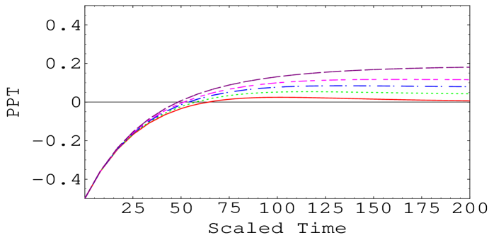
Figure 1: The PPT criterion for the state (3.1), where $p=0,~{}\left\langle\tau_{3}\right\rangle_{eq}=-0.5,~{}\alpha_{i}=T_{1i}/T_{2i}=2.5$ and $\left\langle\sigma_{3}\right\rangle_{eq}=1,0.9,0.8,0.7,0.5$ for the solid, dot, dashed-dot, small-dash and long-dash curves respectively.

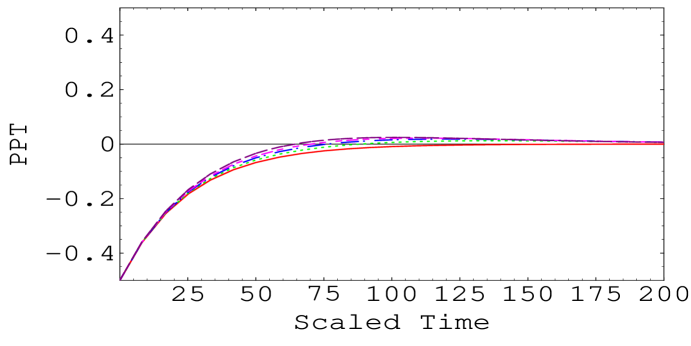
Figure 2: The same as Fig$1$, but for $\left\langle\tau_{3}\right\rangle_{eq}=1$.

The PPT criterion is examined for large values of the absolute equilibrium values of the second qubit, where we consider $\left\langle\tau_{3}\right\rangle_{eq}=1$. In Fig.$2$, the long living entanglement is observed, where the robustness of the output state (3.1) is much better than that depicted in Fig.$1$. Therefore, by increasing the absolute equilibrium values of the two qubits, the living time of entanglement and the robustness of the output state are increased. Furthermore, the phenomena of entanglement-breaking, where the entangled state evolves to a separable state, is observed as one decreases these absolute equilibrium values.

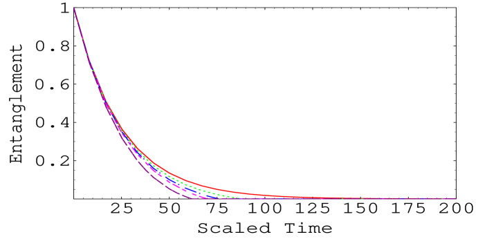
Figure 3: The degree of entanglement where the parameters are the same as Fig$1.$ while $\left\langle\tau_{3}\right\rangle_{eq}=1$.

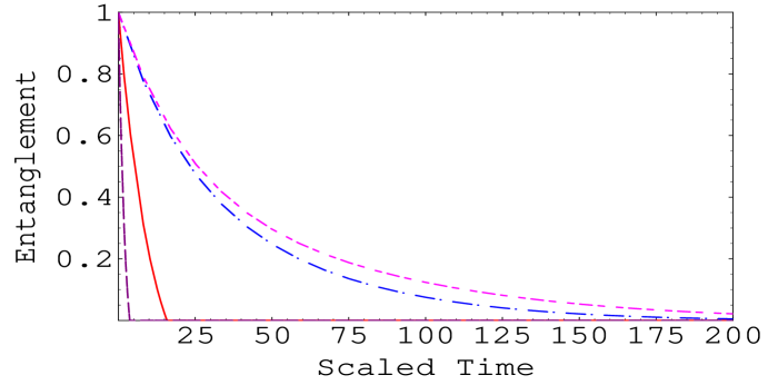
Figure 4: The degree of entanglement for different values of the ratio between the longitudinal and transverse time $\alpha_{i}$. The parameters are $\left\langle\sigma_{3}\right\rangle_{eq}=1,\left\langle\tau_{3}\right\rangle_{eq}=-0.5$ and $\alpha_{i}=2.5,0.5,0.33,0.25$ for the long-dash, solid, dash-dot , and dash-dash curves respectively.

Now, we investigate the effect of the equilibrium values on the survival amount of entanglement for the output state (3.1). For the numerical calculations we consider the case where $\left\langle\tau_{3}\right\rangle_{eq}=-0.5$, $\alpha_{i}=\frac{1}{2},~{}i=1,2$. Fig.$3$, shows the dynamics of entanglement for different values $\left\langle\sigma_{3}\right\rangle_{eq}$. For small values of $\left\langle\sigma_{3}\right\rangle_{eq}$, the degree of entanglement decays faster and the entangled time decreases. On the other hand, the decay of entanglement is smooth and the time of living entanglement increases for larger values of $\left\langle\sigma_{3}\right\rangle_{eq}$.

The dynamic of entanglement for different values the parameter $\alpha_{i}$ is shown in Fig.$4$. It is clear that as $\alpha_{i}$ increases, i.e the longitudinal relaxation time is larger than the transverse relaxation time for both qubits, the entanglement decays much faster as compared with in Fig.$3$. Moreover, the phenomena of the sudden death of entanglement is observed [4, 5].

3.2 Partially entangled states

In this section, we consider a class of non-maximally entangled states. In our calculations we consider a class of partially entangled states with $p=0.5$. Also, we investigate the dynamic of PPT criterion and the degree of entanglement, where we use the same values of the channel parameters.

Fig.$5$, shows the effect of the equilibrium values on the PPT criterion of the output state, where the possibility of considering the Bloch channel as an entanglement-breaking channel decreases and the time of entangled increases. Comparing Fig.$1$ with Fig.$5$, we can see that starting from a partially entangled states the output state is more robust than starting from a maximally entangled state. This means that, the separability and entangled behavior of the input entangled state, not only depend on the channel parameters but also on the structure of the input state.

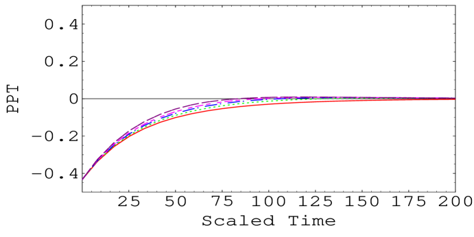
Figure 5: The same as Fig.$(1)$, but for a partially entangled state.

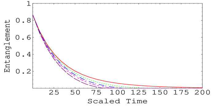
Figure 6: The same as Fig.$(3)$, but for a partially entangled state.

In Fig.$6$, we investigate the dynamics of the entanglement for fixed values of $\left\langle\tau_{3}\right\rangle_{eq}$ and $\alpha_{i}$, and for several values of $\left\langle\sigma_{3}\right\rangle_{eq}$. The general behavior is the same as that shown in Fig.$3$, but the entanglement decays more smoothly and disappears gradually. Therefore the phenomena of sudden death of entanglement does not show for this class of states. Comparing Fig.$3$ and Fig.$6$, shows the time of the lived entanglement is much larger for partially entangled state and the entanglement vanishes gradually. So maximally entangled state is more fragile than partially entangled state.

4 Teleportation

In this section, we examine whether the output state can be used as a quantum channel to achieve teleportation or not. For this task, we use Horodecki’s criterion [20], where any mixed spin $\frac{1}{2}$ state is useful for teleportation if $tr{\sqrt{{\mathord{\begin{picture}(12.0,12.0)(-1.0,0.0)\put(-2.0,10.0){\makebox(0.0,0.0)[t]{$\scriptscriptstyle\downarrow$}} \put(-2.0,11.0){\makebox(0.0,0.0)[l]{$\scriptscriptstyle\longrightarrow$}} \put(5.0,0.0){\makebox(0.0,0.0)[b]{$C$}} \end{picture}}}^{\raisebox{-1.0pt}{\scriptsize{T}}}\mathord{\begin{picture}(12.0,12.0)(-1.0,0.0)\put(-2.0,10.0){\makebox(0.0,0.0)[t]{$\scriptscriptstyle\downarrow$}} \put(-2.0,11.0){\makebox(0.0,0.0)[l]{$\scriptscriptstyle\longrightarrow$}} \put(5.0,0.0){\makebox(0.0,0.0)[b]{$C$}} \end{picture}}}}>1$. By using this criterion, we find that, the output state which is defined by (3) and (3) is available for quantum teleportation if the following inequality is obeyed

Telp $$= 2q^{2}\beta_{1}^{2}\beta_{2}^{2}+\bigl{[}(1-\gamma_{1})(1-\gamma_{2})\left\langle\sigma_{3}\right\rangle_{eq}\left\langle\tau_{3}\right\rangle_{eq}$$ (18)

$$+ p\left(\gamma_{1}(1-\gamma_{2})\left\langle\tau_{3}\right\rangle_{eq}-\gamma_{2}(1-\gamma_{1})\left\langle\sigma_{3}\right\rangle_{eq}\right)-\gamma_{1}\gamma_{2}\bigr{]}^{2}>1.$$

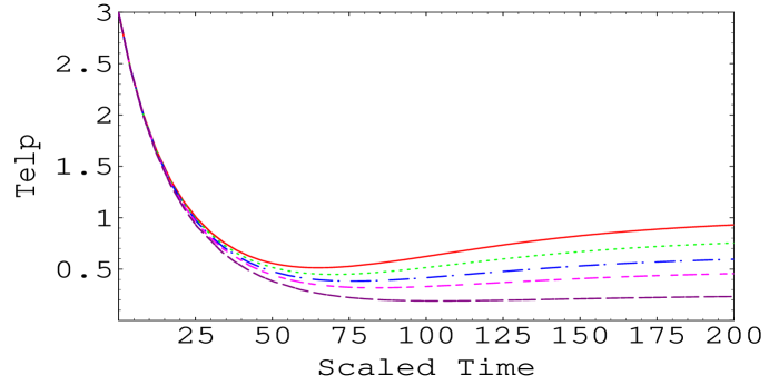
Figure 7: The teleportation inequality (18), where the parameters are the same as Fig.$1$. (a)for the maximally entangled state and (b) for the partially entangled state.

Fig.$7a$, shows the behavior of the teleportation inequality (18) for the output state (3.1). It is clear that as the absolute equilibrium values increase, the possibility of using this channel for quantum teleportation increases. As an example for $\left\langle\sigma_{3}\right\rangle_{eq}=1$, the time interval in which the teleportation inequality obeyed is $[0,25.2]$, while it is $[0,23.1]$ for $\left\langle\sigma_{3}\right\rangle_{eq}=0.5$.

In Fig.$7b$, we plot the teleportation inequality for the output state with $p=0.5$, i.e the partial entangled class. In general, the behavior of the teleportation inequality is the same as that depicted in Fig.$7b$, but the time to use the state as a quantum channel to perform teleportation is larger. As an example, for $\left\langle\sigma_{3}\right\rangle_{eq}=1$ the teleportation inequality is obeyed in the time interval $[0,30.9]$. This is due to that the output state for a system prepared initially in a partially entangled state is more robust than that obtained from a system initially prepared in a maximum entangled state.

At this end, we achieve the quantum teleportation by using the output state as a quantum channel. Assume that Alice is given an unknown state defined by its state vector

$$\bigl{|}\Psi\bigr{\rangle}=\lambda_{1}\bigl{|}0\bigr{\rangle}+\lambda_{2}\bigl{|}1\bigr{\rangle},$$ (19)

where $\lambda^{2}_{1}+\lambda^{2}_{2}=1$. Now she wants to sent this state to Bob through their quantum channel. To attain this aim , Alice and Bob will use the original teleportation protocol [21]. In this case the total state of the system is $\rho_{\psi}\otimes\rho^{out}$, where $\psi$ is given by (19) and $\rho^{out}$ is defined by (3) and (3). Alice makes a measurement on the given qubit and her own qubit. Then she sends her results through a classical channel to Bob. As soon as Bob receives the classical data, he performs a suitable unitary operation on his qubit and gets the teleported state. If Alice measures the Bell state, $\bigl{|}\phi^{+}\bigr{\rangle}\bigl{\langle}\phi^{+}\bigr{|}=\frac{1}{\sqrt{2}}(\bigl{|}00\bigr{\rangle}+\bigl{|}11\bigr{\rangle})$, then the final state at Bob’s hand is

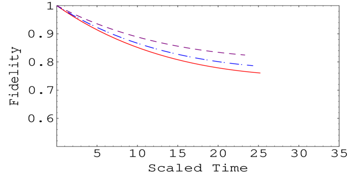
Figure 8: The fidelity for (a) Maximally entangled state and (b) Partially entangled stat, where $\left\langle\sigma_{3}\right\rangle_{eq}=1,0.8,0.5.$ for the solid, dash-dot and dot curves respectively, with $\alpha_{i}=0.5$, $\lambda_{1}=1$ and $\left\langle\tau_{3}\right\rangle=-1$.

$$\rho_{Bob}=\eta_{1}\bigl{|}0\bigr{\rangle}\bigl{\langle}0\bigr{|}+\eta_{2}\bigl{|}0\bigr{\rangle}\bigl{\langle}1\bigr{|}+\eta_{3}\bigl{|}1\bigr{\rangle}\bigl{\langle}0\bigr{|}+\eta_{4}\bigl{|}1\bigr{\rangle}\bigl{\langle}1\bigr{|},$$ (20)

where,

$$\eta_{1} = \frac{1}{2}\biggl{[}|\lambda_{1}|^{2}(1+\tilde{A}_{3}(t)-\tilde{B}_{3}(t)-\tilde{C}_{33}(t))+|\lambda_{2}|^{2}(1-\tilde{A}_{3}(t)+\tilde{B}_{3}(t)+\tilde{C}_{33}(t))\biggr{]},$$

$$\eta_{2} = \frac{1}{2}\left[\lambda_{1}\lambda^{*}_{2}(\tilde{C}_{11}(t)-\tilde{C}_{22}(t))+\lambda_{1}^{*}\lambda_{2}(\tilde{C}_{11}(t)+\tilde{C}_{22}(t))\right],$$

$$\eta_{3} = \frac{1}{2}\left[\lambda_{1}\lambda^{*}_{2}(\tilde{C}_{11}(t)+\tilde{C}_{22}(t))+\lambda_{1}^{*}\lambda_{2}(\tilde{C}_{11}(t)-\tilde{C}_{22}(t))\right],$$

$$\eta_{4} = \frac{1}{2}\biggl{[}|\lambda_{1}|^{2}(1+\tilde{A}_{3}(t)+\tilde{B}_{3}(t)+\tilde{C}_{33}(t))+|\lambda_{2}|^{2}(1-\tilde{A}_{3}(t)+\tilde{B}_{3}(t)-\tilde{C}_{33}(t))\biggr{]},$$

The fidelity, $F$, of the teleported state is

$$F=|\lambda_{1}|^{2}\eta_{1}+\lambda_{1}\lambda_{2}^{*}\eta_{2}+\lambda_{1}^{*}\lambda_{2}\eta_{3}+|\lambda_{2}|^{2}\eta_{4}.$$ (22)

In Fig$.8$, we plot the fidelity of the teleported state at Bob’s hand. When the maximally entangled state is used as a quantum channel between Alice and Bob, the fidelity of the teleported state is shown in Fig.$8a$. It is clear that, the fidelity decreases as one increases the absolute equilibrium values. This is due to the decay of the degree of entanglement. On the other hand, since the entanglement survives for a long time, the output state can be used to achieve quantum teleportation for a long time. Fig.$(8b)$, shows the behavior of the fidelity of the teleported state when the output state with $p=0.5$ is used as a channel. The teleported time, the time which one can use the output state as channel, increases and the fidelity is better than that shown in Fig.$(8a)$.

5 Conclusion

In this contribution, we have investigated analytically the dynamics of a two-qubit state passes through a Bloch channel. We have discussed the influence of the Bloch channel’s parameters on the separability and entangled behavior of the output state. The results show that, the robustness of the entangled qubit pairs increases as one increases the absolute values of the equilibrium parameters or decreases the ratio of the longitudinal and transverse relaxation times.

The amount of entanglement contained in the output state is quantified, where we have shown that it is fragile for maximum entangled states and robust for partial entangled states. The phenomena of the decay and the sudden death of entanglement are observed for these types of systems.

Moreover the ability of performing quantum teleportation by using the output state is examined. It is found that for large absolute equilibrium values, the output state is more useful for quantum teleportation. Furthermore, the intervals of time in which the state is available for performing teleportation increase. The original teleportation protocol is performed by using the output state as a channel between Alice and Bob. From our results, we see that the fidelity of the teleported state increases as one decreases the equilibrium values of the two qubits, but the time in which the state is useful for quantum teleportation decreases.

References

[1]
H.-J.Briegel, W. Dür, J. I. Cirac Phys. Rev. Lett.81 5932 (1998); W. Dür, H.-J. Briegel, J. I. Cirac, Phys.
Rev. A 59 196 (1999); N. Gisin, G. Ribordy, W. Tittel, Rev.
of Mod. Phys.74 145 (2002).
[2]
H. Zhengang, X. Zuhong and Y. Zhang, Phys. Lett. A354, 79 ((2006));
H. Prakash, N. Chandra, R. Prakash and Shivani,
J. Phys. B40 1613 (2007).
[3]
S. Luo, J. Phys. A38,2991 (2005); S. Zheng, J. Phys.
B39 4147 (2006).
[4]
T. Yu and J. H. Eberly, Opt. Commu.264 393 (2006); M.
Yonac, T. Yu and J. H. Eberly, J. Phys. B39 S621 (2006);
T Yu and J. H. Eberly; J. Mod. Opt. 54, 2289-2296 (2007).
[5]
L. Aolita, R. Chaves, D. Cavalcanti, A. Acin and L. Davidovich
Phys. Rev. Lett.100 080501 (2008).
[6] G. Pineda, T.
Gorin and T. H. Seligman, New Journal of Physics 9 106 (2007).
[7]
G. M. Palma, K. -A. Suominen and A. K. Ekert, Proc. R. Soc. London
A452 567 (1996).
[8] B.Georgot and D. L. Shepelyansky, Phys. Rev.E 62 3504 (2000).
[9]
M. Sugahara, S. P.Kruchinin, Mod. Phys. Lett. B15 473
(2001).
[10]
M. Ban, F. Shibata, S. Kitajima, J. Phys. B40 1613 (2007); X.
San Ma, An. Min Wang, Opt. Commu.270 465 (2007).
[11]
M. Ban, S. Kitajima abd F. Shibata, J. Phys. A38 4235 (2005).
[12]
M. Ban, S. Kitajima abd F. Shibata, J. Phys. A38 7161 (2005);
[13]
G. Mahler and V. A. Weberruß” Quantum Networks: Dynamics of Open
Nanostructures” Springer-Verlag, 1998”
[14]
B.-G. Englert and N. Metwally, J. Mod. Opt. 47, 221 (2000); N. Metwally,
M. R. B. Wahiddin and M. Bourennane, Opt. Commu.257 206
(2006).
[15]
X. Cui, S.-J. Gu, J. Cao and Y. Wang, J. Phys. A 40 13523-13533
(2007).
[16]F. Benatti, R. Floreanini and R. Romano,
J. Phys. A 35 4955 (2002); S. Daffer, K. Wodkiewicz and J.
Mclver, Phys. Rev. A 70, 010304 (2004).
[17]
B.-G. Englert and N. Metwally, App. Phys. B72 55(2001).
[18]
A. Peres, Phys. Rev. Lett. 77 1413 1996; R.Horodecki, M.
Horodecki and P. Horodecki, Phys. Lett. A222, 1 (1996).
[19]
K. Zyczkowski, P. Horodecki, A. Sanpera and M. Lewenstein,
Phys. Rev. A 58, 883 (1998).
[20]
P. Horodecki, Phys. Lett. A232, 333 (1997).
[21]
C. H. Bennett, G. Brassard, C. Crepeau, R. Jozsa, A. Peres and W. K. Wottors, Phys.
Rev. Lett 70,1895 (1993).